Dark Matter Particle Candidatesdark matter simulations, which have not been carried out...

Paolo Gondolo University of Utah

Dark Matter Particle Candidates

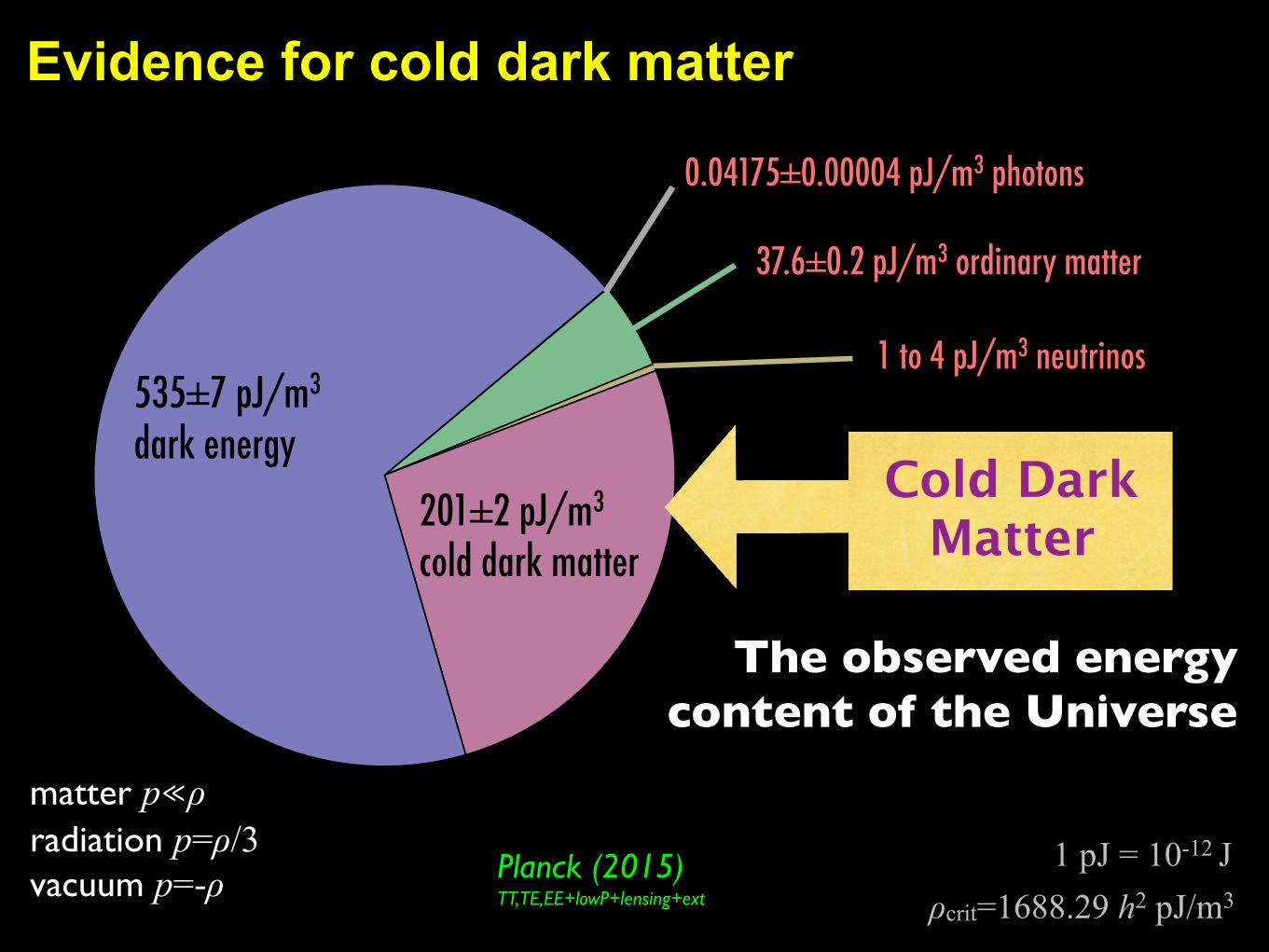
Evidence for cold dark matter

37.6±0.2 pJ/m3 ordinary matter

1 to 4 pJ/m3 neutrinos

201±2 pJ/m3 cold dark matter

535±7 pJ/m3 dark energy

0.04175±0.00004 pJ/m3 photons

Planck (2015) TT,TE,EE+lowP+lensing+ext

matter p≪ρradiation p=ρ/3 vacuum p=-ρ

1 pJ = 10-12 Jρcrit=1688.29 h2 pJ/m3

The observed energy content of the Universe

Cold Dark Matter

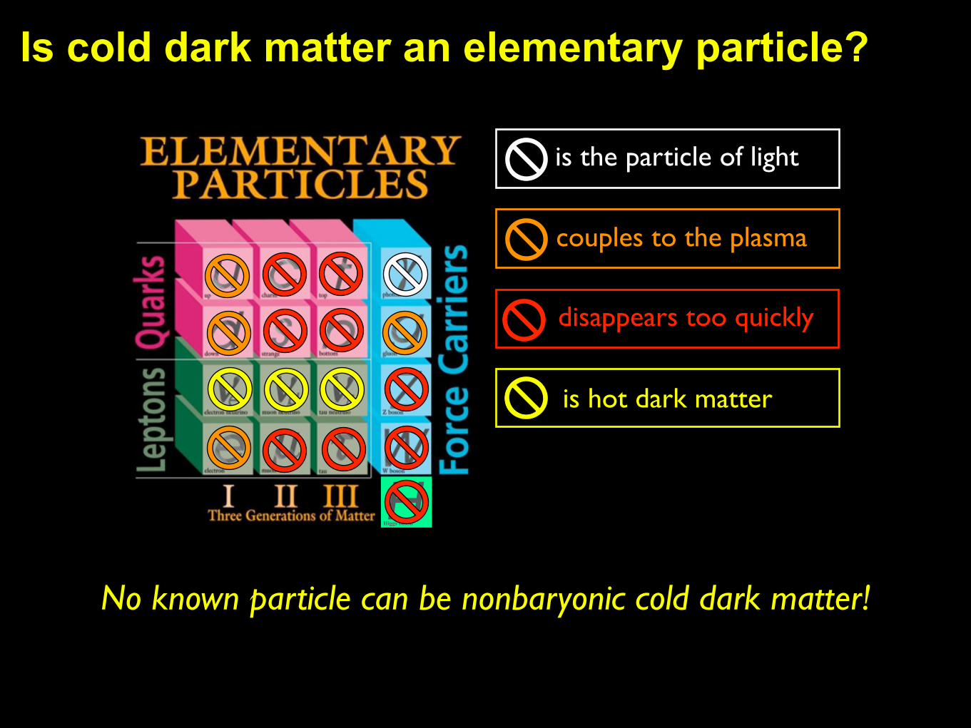
Is cold dark matter an elementary particle?

disappears too quickly

couples to the plasma

is hot dark matter

is the particle of light

No known particle can be nonbaryonic cold dark matter!

HHiggs boson

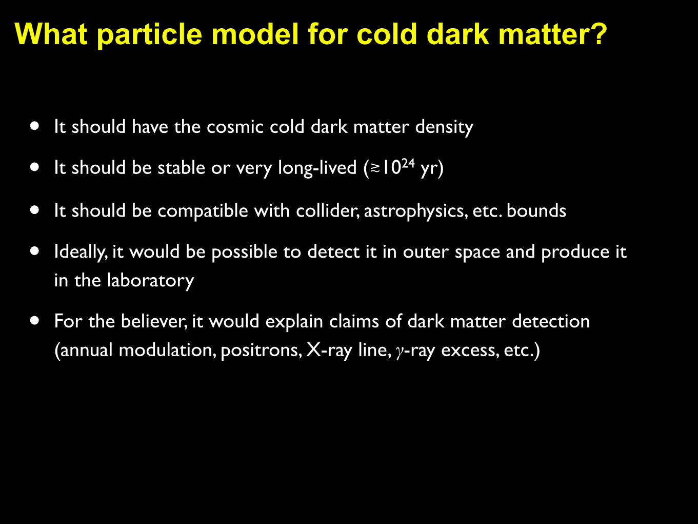
What particle model for cold dark matter?

• It should have the cosmic cold dark matter density

• It should be stable or very long-lived (≳1024 yr)

• It should be compatible with collider, astrophysics, etc. bounds

• Ideally, it would be possible to detect it in outer space and produce it in the laboratory

• For the believer, it would explain claims of dark matter detection (annual modulation, positrons, X-ray line, γ-ray excess, etc.)

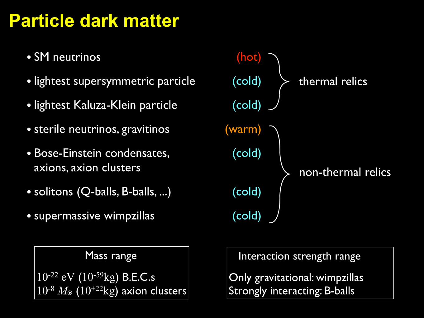
Particle dark matter

(hot)

(cold)

(cold)

(warm)

(cold)

(cold)

(cold)

thermal relics

non-thermal relics

• SM neutrinos

• lightest supersymmetric particle

• lightest Kaluza-Klein particle

• sterile neutrinos, gravitinos

• Bose-Einstein condensates, axions, axion clusters

• solitons (Q-balls, B-balls, ...)

• supermassive wimpzillas

Mass range

10-22 eV (10-59kg) B.E.C.s10-8 M⦿ (10+22kg) axion clusters

Interaction strength range

Only gravitational: wimpzillasStrongly interacting: B-balls


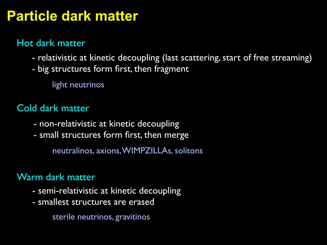
Hot dark matter

Cold dark matter

- relativistic at kinetic decoupling (last scattering, start of free streaming)- big structures form first, then fragment

light neutrinos

neutralinos, axions, WIMPZILLAs, solitons

Warm dark matter

- non-relativistic at kinetic decoupling- small structures form first, then merge

- semi-relativistic at kinetic decoupling- smallest structures are erased

sterile neutrinos, gravitinos


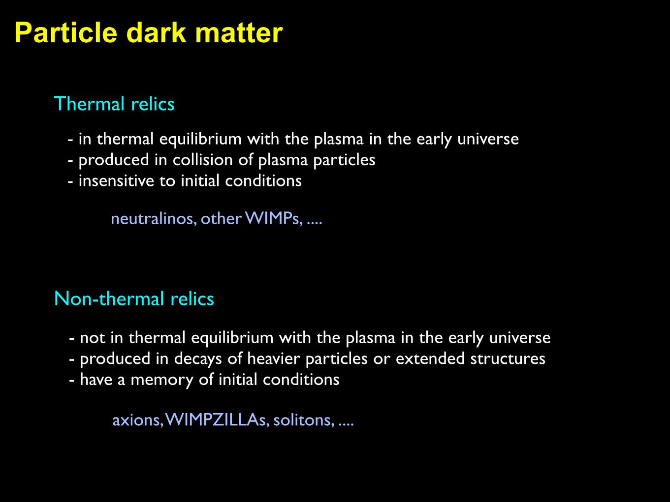
Thermal relics

Non-thermal relics

neutralinos, other WIMPs, ....

axions, WIMPZILLAs, solitons, ....

- in thermal equilibrium with the plasma in the early universe- produced in collision of plasma particles- insensitive to initial conditions

- not in thermal equilibrium with the plasma in the early universe- produced in decays of heavier particles or extended structures- have a memory of initial conditions

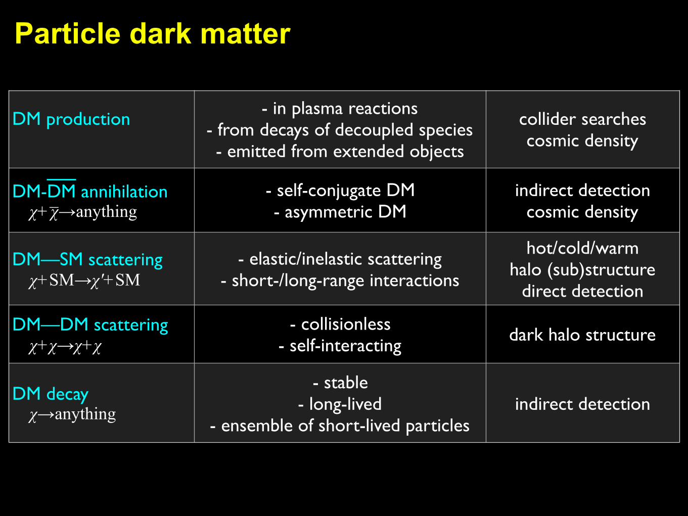
DM production - in plasma reactions- from decays of decoupled species- emitted from extended objects

collider searchescosmic density

DM-DM annihilation χ+ χ̅→anything

- self-conjugate DM- asymmetric DM

indirect detectioncosmic density

DM—SM scattering χ+SM→χ′+SM

- elastic/inelastic scattering- short-/long-range interactions

hot/cold/warmhalo (sub)structure

direct detection

DM—DM scattering χ+χ→χ+χ

- collisionless- self-interacting dark halo structure

DM decay χ→anything

- stable - long-lived

- ensemble of short-lived particlesindirect detection


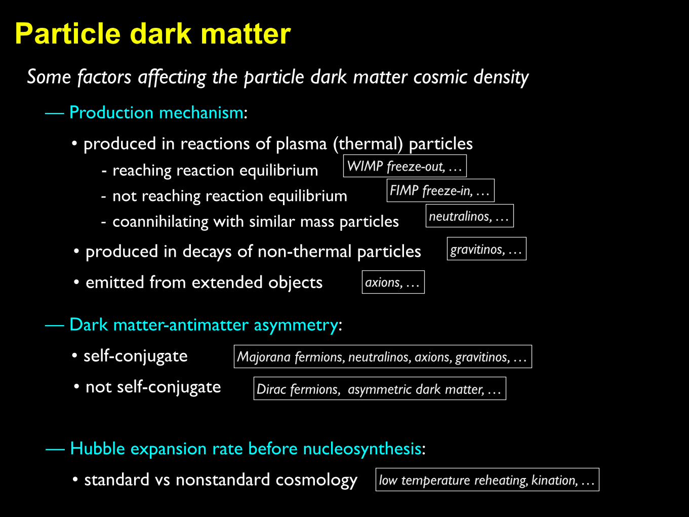
Particle dark matterSome factors affecting the particle dark matter cosmic density

— Dark matter-antimatter asymmetry:

• self-conjugate

• not self-conjugate

Majorana fermions, neutralinos, axions, gravitinos, …

Dirac fermions, asymmetric dark matter, …

— Hubble expansion rate before nucleosynthesis:

• standard vs nonstandard cosmology low temperature reheating, kination, …

— Production mechanism:

• produced in reactions of plasma (thermal) particles- reaching reaction equilibrium

- not reaching reaction equilibrium

- coannihilating with similar mass particles

• produced in decays of non-thermal particles

• emitted from extended objects

WIMP freeze-out, …

FIMP freeze-in, …

gravitinos, …

axions, …

neutralinos, …

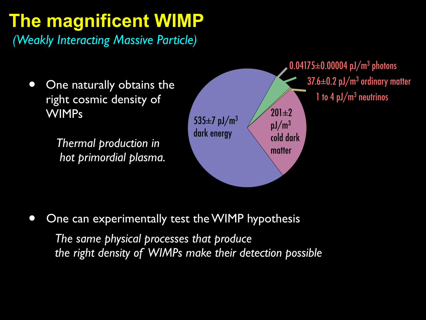
• One naturally obtains the right cosmic density of WIMPs Thermal production in hot primordial plasma.

• One can experimentally test the WIMP hypothesis

The same physical processes that produce the right density of WIMPs make their detection possible

37.6±0.2 pJ/m3 ordinary matter1 to 4 pJ/m3 neutrinos

201±2 pJ/m3 cold dark matter

535±7 pJ/m3 dark energy

0.04175±0.00004 pJ/m3 photons

(Weakly Interacting Massive Particle)The magnificent WIMP

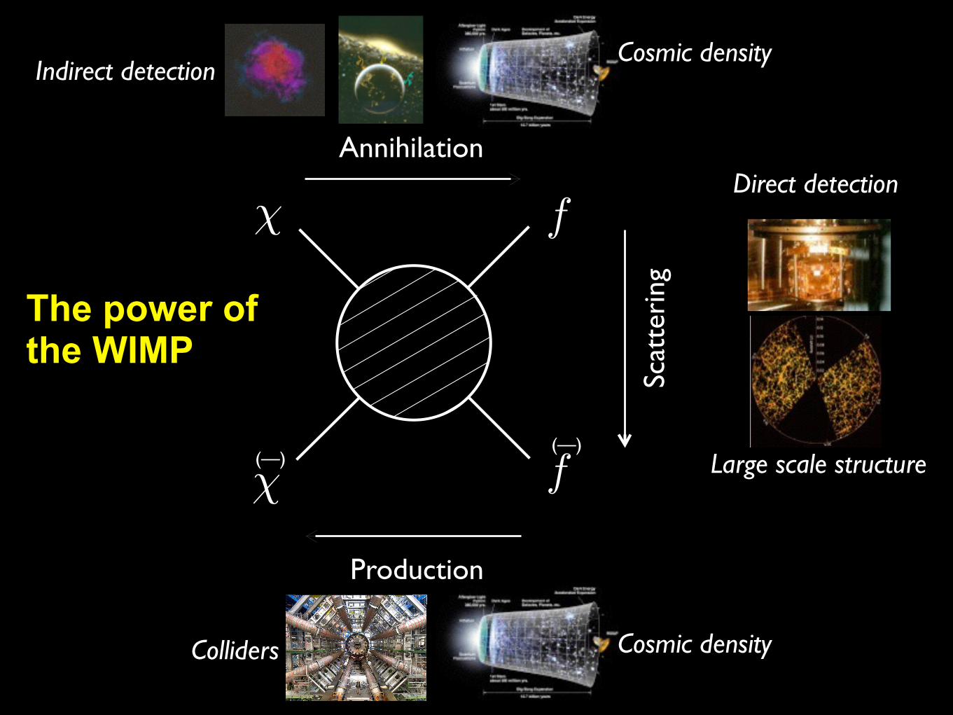
Scat

teri

ng

f�

�(—) f

(—)

Production

AnnihilationDirect detection

Large scale structure

Cosmic densityIndirect detection

Cosmic density

Børge Kile Gjelsten, University of Oslo 44 IDM, Aug 2008

Colliders

The power of the WIMP

Neutrinos

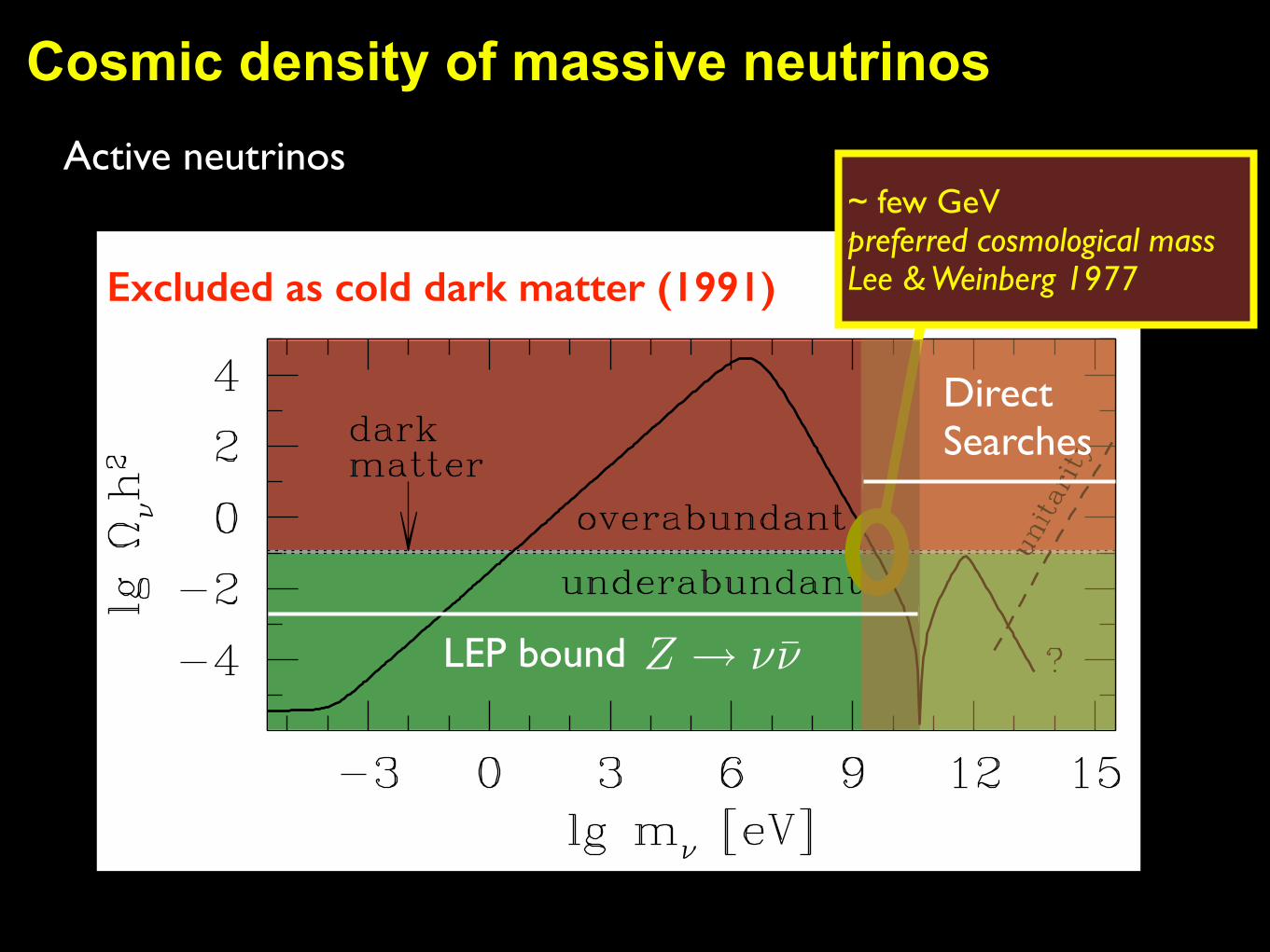
Cosmic density of massive neutrinosActive neutrinos

Excluded as cold dark matter (1991)

~ few GeV preferred cosmological mass Lee & Weinberg 1977

DirectSearches

LEP bound Z ! ⌫⌫̄

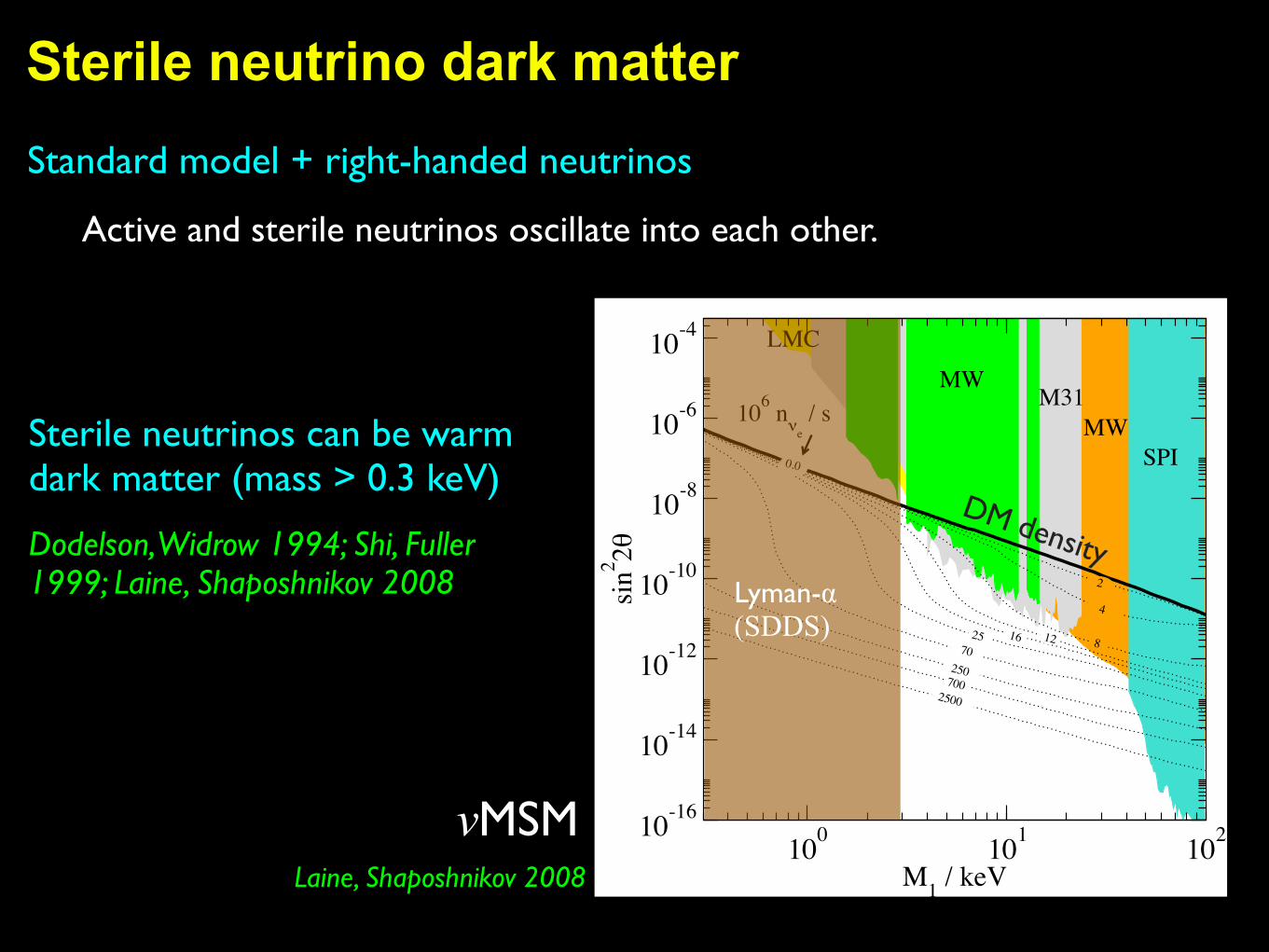
Sterile neutrino dark matterStandard model + right-handed neutrinos

Active and sterile neutrinos oscillate into each other.

Sterile neutrinos can be warm dark matter (mass > 0.3 keV)

Dodelson, Widrow 1994; Shi, Fuller 1999; Laine, Shaposhnikov 2008

100 101 102

M1 / keV

10-16

10-14

10-12

10-10

10-8

10-6

10-4

sin2 2θ

case 1

LMC

MW

MWM31106 nνe

/ s

2

4

81216

0.0

2500

25

250

SPI

70

700

100 101 102

M1 / keV

10-16

10-14

10-12

10-10

10-8

10-6

10-4

sin2 2θ

case 2

LMC

MW

MWM31106 n

νe / s

2

4

81216

0.0

2500

25

250

SPI

70

700

Figure 4: The central region of Fig. 3, M1 = 0.3 . . .100.0 keV, compared with regions excludedby various X-ray constraints [22, 25, 30, 31], coming from XMM-Newton observations of the LargeMagellanic Cloud (LMC), the Milky Way (MW), and the Andromeda galaxy (M31). SPI marks theconstraints from 5 years of observations of the Milky Way galactic center by the SPI spectrometer onboard the Integral observatory.

dark matter simulations, which have not been carried out with actual non-equilibrium spec-

tra so far. Nevertheless, adopting a simple recipe for estimating the non-equilibrium effects

(cf. Eq. (5.1)), the results of refs. [34, 35] can be re-interpreted as the constraints M1 >∼ 11.6

keV and M1 >∼ 8 keV, respectively (95% CL), at vanishing asymmetry [12]. Very recently

limits stronger by a factor 2–3 have been reported [36]. We return to how the constraints

change in the case of a non-zero lepton asymmetry in Sec. 5. We note, however, that the

most conservative bound, the so-called Tremaine-Gunn bound [52, 53], is much weaker and

reads M1 >∼ 0.3 keV [54], which we have chosen as the lower end of the horizontal axes in

Figs. 4, 6.

In Fig. 5 we show examples of the spectra, for a relatively small mass M1 = 3 keV (like

in Fig. 1), at which point the significant changes caused by the asymmetry can be clearly

identified. The general pattern to be observed in Fig. 5 is that for a small asymmetry, the

distribution function is boosted only at very small momenta. Quantities like the average

momentum ⟨q⟩s then decrease, as can be seen in Fig. 6. For large asymmetry, the resonance

affects all q; the total abundance is strongly enhanced with respect to the case without a

resonance, but the shape of the distribution function is less distorted than at small asymmetry,

so that the average momentum ⟨q⟩s returns back towards the value in the non-resonant case.

Therefore, for any given mass, we can observe a minimal value of ⟨q⟩s in Fig. 6, ⟨q⟩s >∼ 0.3⟨q⟩a.This minimal value is remarkably independent of M1, but the value of asymmetry at which

15

DM densityLyman-α(SDDS)

νMSMLaine, Shaposhnikov 2008

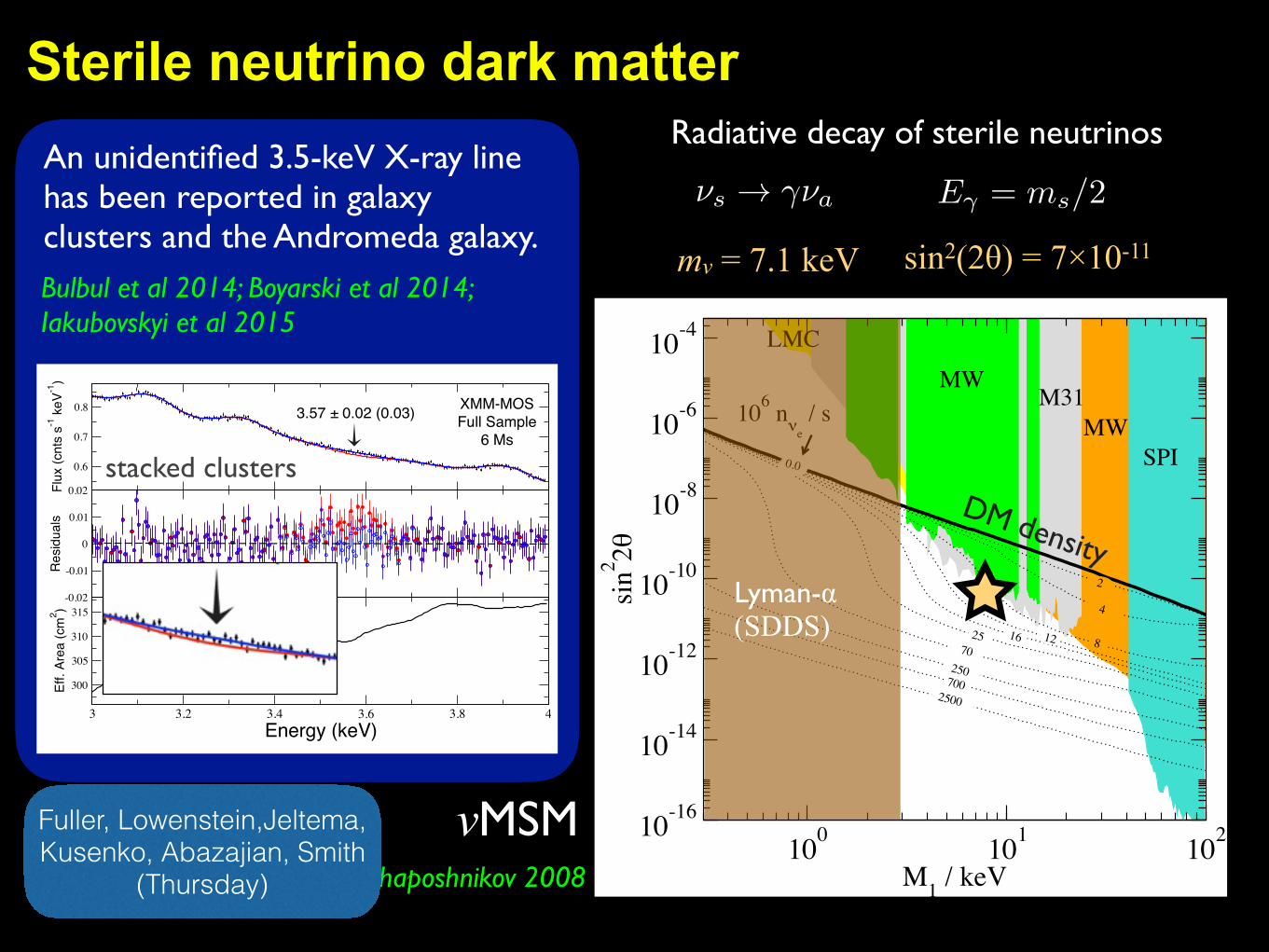
Sterile neutrino dark matterAn unidentified 3.5-keV X-ray line has been reported in galaxy clusters and the Andromeda galaxy.

100 101 102

M1 / keV

10-16

10-14

10-12

10-10

10-8

10-6

10-4

sin2 2θ

case 1

LMC

MW

MWM31106 nνe

/ s

2

4

81216

0.0

2500

25

250

SPI

70

700

100 101 102

M1 / keV

10-16

10-14

10-12

10-10

10-8

10-6

10-4

sin2 2θ

case 2

LMC

MW

MWM31106 n

νe / s

2

4

81216

0.0

2500

25

250

SPI

70

700

Figure 4: The central region of Fig. 3, M1 = 0.3 . . .100.0 keV, compared with regions excludedby various X-ray constraints [22, 25, 30, 31], coming from XMM-Newton observations of the LargeMagellanic Cloud (LMC), the Milky Way (MW), and the Andromeda galaxy (M31). SPI marks theconstraints from 5 years of observations of the Milky Way galactic center by the SPI spectrometer onboard the Integral observatory.

dark matter simulations, which have not been carried out with actual non-equilibrium spec-

tra so far. Nevertheless, adopting a simple recipe for estimating the non-equilibrium effects

(cf. Eq. (5.1)), the results of refs. [34, 35] can be re-interpreted as the constraints M1 >∼ 11.6

keV and M1 >∼ 8 keV, respectively (95% CL), at vanishing asymmetry [12]. Very recently

limits stronger by a factor 2–3 have been reported [36]. We return to how the constraints

change in the case of a non-zero lepton asymmetry in Sec. 5. We note, however, that the

most conservative bound, the so-called Tremaine-Gunn bound [52, 53], is much weaker and

reads M1 >∼ 0.3 keV [54], which we have chosen as the lower end of the horizontal axes in

Figs. 4, 6.

In Fig. 5 we show examples of the spectra, for a relatively small mass M1 = 3 keV (like

in Fig. 1), at which point the significant changes caused by the asymmetry can be clearly

identified. The general pattern to be observed in Fig. 5 is that for a small asymmetry, the

distribution function is boosted only at very small momenta. Quantities like the average

momentum ⟨q⟩s then decrease, as can be seen in Fig. 6. For large asymmetry, the resonance

affects all q; the total abundance is strongly enhanced with respect to the case without a

resonance, but the shape of the distribution function is less distorted than at small asymmetry,

so that the average momentum ⟨q⟩s returns back towards the value in the non-resonant case.

Therefore, for any given mass, we can observe a minimal value of ⟨q⟩s in Fig. 6, ⟨q⟩s >∼ 0.3⟨q⟩a.This minimal value is remarkably independent of M1, but the value of asymmetry at which

15

DM densityLyman-α(SDDS)

νMSMLaine, Shaposhnikov 2008

Radiative decay of sterile neutrinos

mν = 7.1 keV sin2(2θ) = 7×10-11

Bulbul et al 2014; Boyarski et al 2014; Iakubovskyi et al 2015

0.6

0.7

0.8

Flu

x (

cn

ts s

-1 k

eV

-1)

-0.02

-0.01

0

0.01

0.02

Re

sid

ua

ls

3 3.2 3.4 3.6 3.8 4Energy (keV)

300

305

310

315

Eff

. A

rea

(cm

2)

3.57 ± 0.02 (0.03)XMM-MOS

Full Sample

6 Ms

stacked clusters

E� = ms/2⌫s ! �⌫a

Fuller, Lowenstein,Jeltema, Kusenko, Abazajian, Smith

(Thursday)

Neutralinos

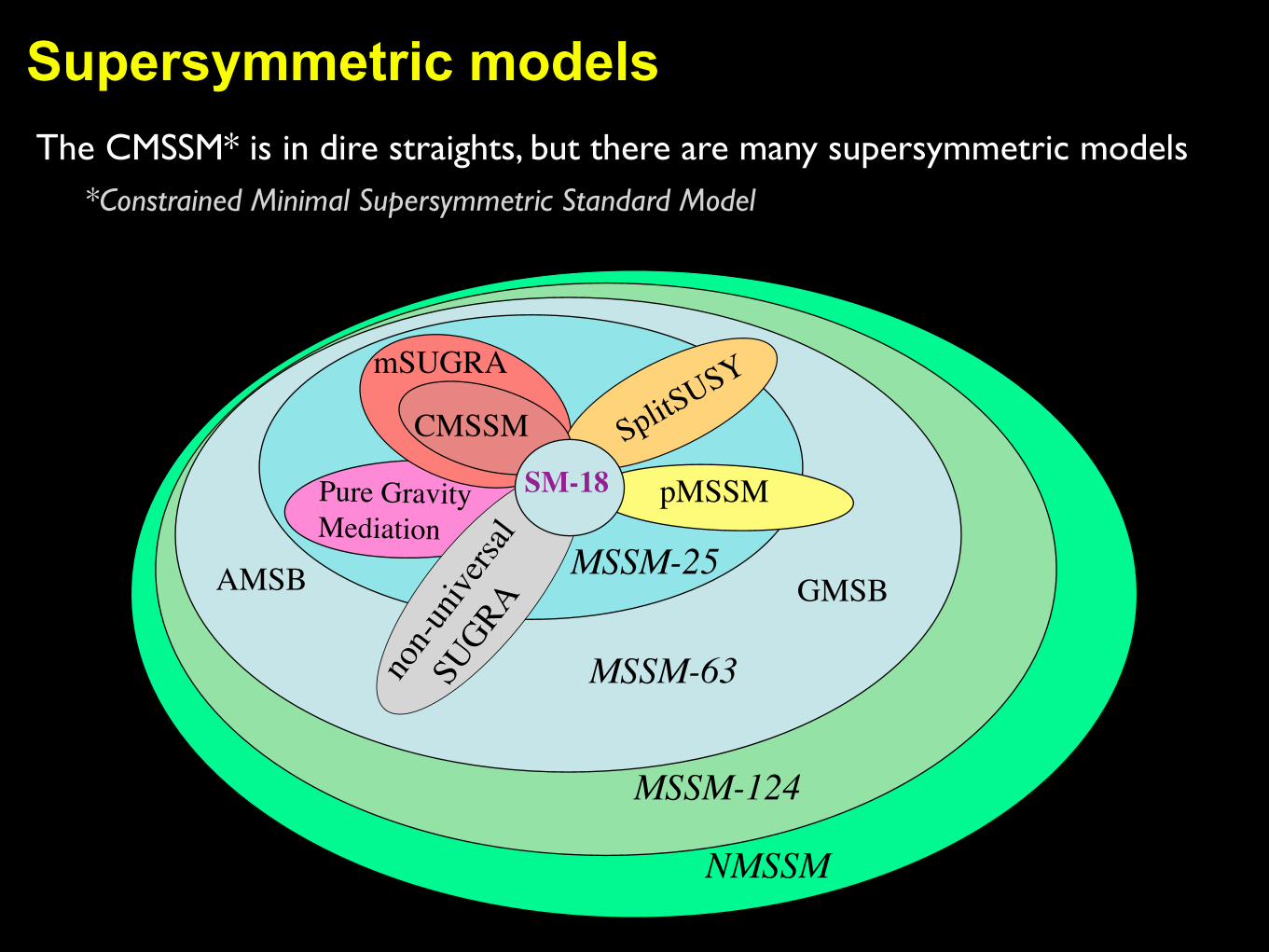
mSUGRA

AMSB

SplitSUSY

non-u

nivers

al

SUGRA

NMSSM

GMSBMSSM-25

MSSM-63

MSSM-124

SM-18 pMSSM

CMSSM

Pure Gravity Mediation

*Constrained Minimal Supersymmetric Standard Model

The CMSSM* is in dire straights, but there are many supersymmetric models

Supersymmetric models

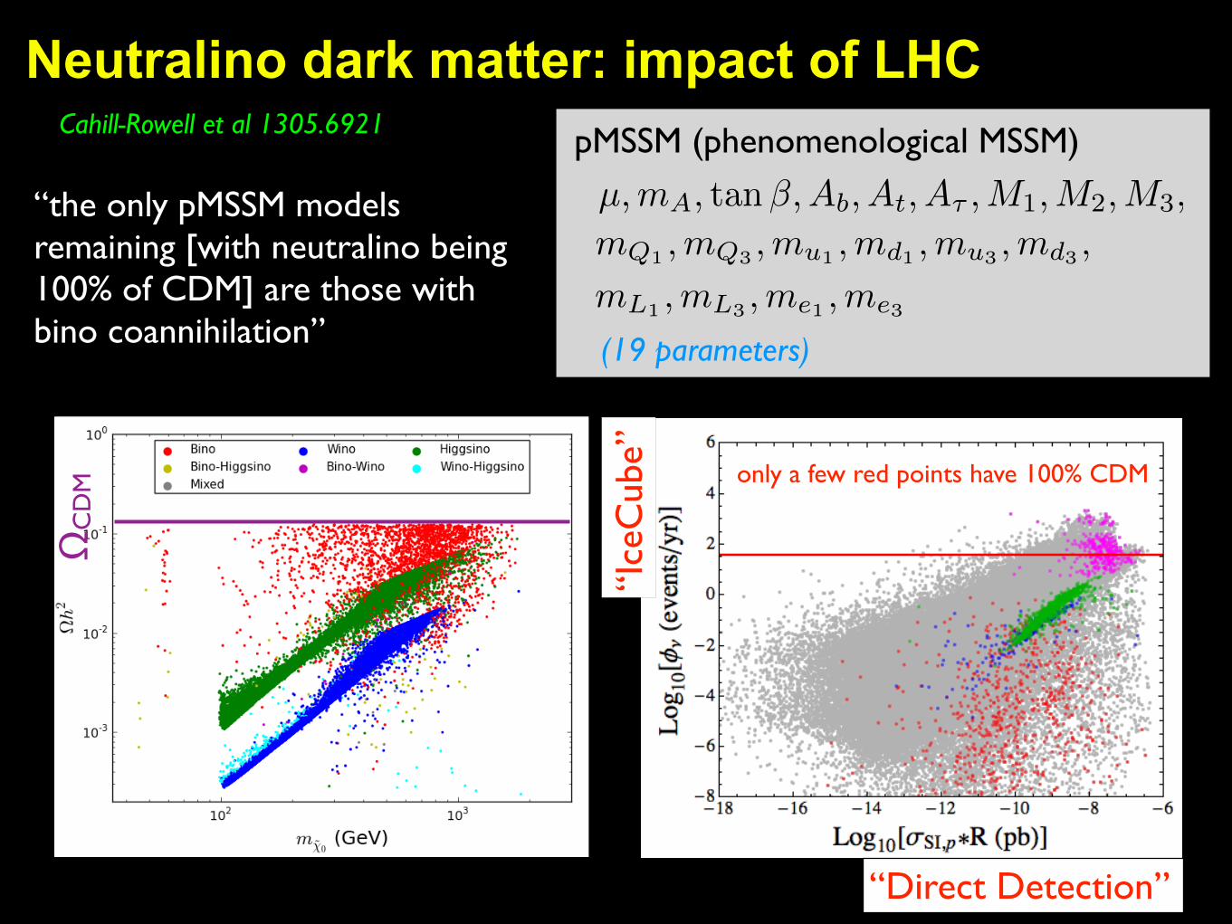
Cahill-Rowell et al 1305.6921

Neutralino dark matter: impact of LHC

“the only pMSSM models remaining [with neutralino being 100% of CDM] are those with bino coannihilation”

are highly detectable by IC/DC. We observe that all such WMAP-saturating well-temperedneutralinos with masses mLSP 500GeV should be excluded by the IC/DC search (c.f., themagenta points in Fig. 8).

Figure 8: IC/DC signal event rates as a function of LSP mass (upper-left), thermal annihi-lation cross-section h��iR2 (upper-right) and thermal elastic scattering cross-sections �SD,p

and �SI,p (lower panels). In all panels the gray points represent generic models in our fullpMSSM model set, while WMAP-saturating models with mostly bino, wino, Higgsino ormixed (80% of each) LSPs in are highlighted in red, blue, green and magenta, respectively.The red line denotes a detected flux of 40 events/yr, our conservative estimate for exclusion.

6 Complementarity: Putting It All Together

Now that we have provided an overview of the various pieces of data that go into our analysis,we can put them together to see what they (will) tell us about the nature of the neutralino

16

densities. Of course, even for masses up to 1-2 TeV, XENON1T still provides quite decentmodel coverage in this parameter plane. As noted already, most of the impact of the LHC isat present seen to be at lower LSP masses below ⇠ 500 GeV. The LHC coverage is relativelyuniform as far as the value of the relic density is concerned except in the case of very lightLSPs where the coverage is very strong. Of course, we again remind the reader that westill need to add the additional information coming from the new 8 TeV LHC analyses notincluded here as well as the extrapolations to 14 TeV so that the coverage provided by theLHC should be expected to improve substantially.

Figure 13: Thermal relic density as a function of the LSP mass for all pMSSM models,surviving after all searches, color-coded by the electroweak properties of the LSP. Comparewith Fig. 2.

Finally, Fig. 13 shows the impact of combining all of the di↵erent searches in this same⌦h2-LSP mass plane which should be compared with that for the original model set asgenerated that is shown in Fig. 2. Here we see that (i) the models that were in the light h

23

“Ice

Cub

e”

ΩC

DM

“Direct Detection”

only a few red points have 100% CDM

pMSSM (phenomenological MSSM)

µ,mA, tan�, Ab, At, A⌧ ,M1,M2,M3,mQ1 ,mQ3 ,mu1 ,md1 ,mu3 ,md3 ,

mL1 ,mL3 ,me1 ,me3

(19 parameters)

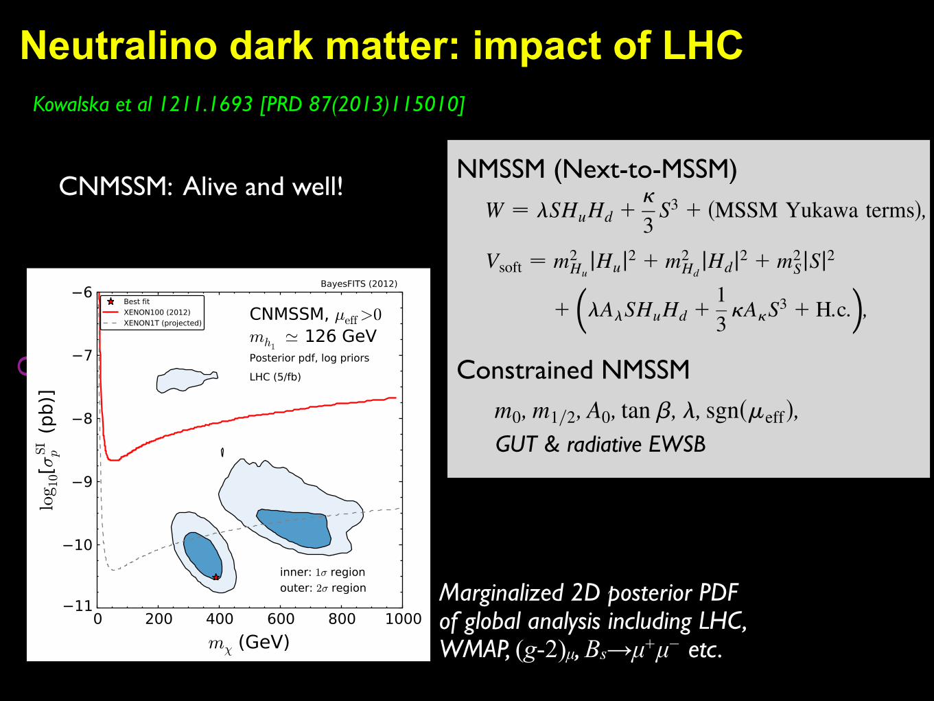
Kowalska et al 1211.1693 [PRD 87(2013)115010]

Neutralino dark matter: impact of LHC

CNMSSM: Alive and well!

ΩC

DM

the posterior distribution. For the same reason Rh1ðZZÞcannot be perfectly fitted either, though its contributionto the total !2 is smaller than 0.5 units of !2, making thisobservable equally ineffective in constraining theposterior.

In Fig. 9(b) we present the posterior distribution forcase 2. Once again, Rh2ð""Þ can hardly become largerthan 1 over the preferred parameter space. The 95% cred-ible region lies far from the central value of the observedenhancement and, in fact, even covers values lower than incase 1. Rh2ðZZÞ presents similar behavior, although thesuppression of the reduced cross section is highly welcomefor this observable, as it places the calculated value closerto the rate observed at CMS. Smaller than 1 signal ratesindicate less of a SM-like character for h2, which is causedby the suppression of the SM couplings induced by itsincreased singlet component.

The posterior distributions presented in Figs. 9(a) and9(b) indicate that, in both case 1 and case 2 it is ingeneral extremely difficult to obtain the signal enhance-ment in the "" channel. The scan naturally tends to stayin the regions of parameter space favored by all con-straints. It is therefore no surprise that among the pointsscanned for case 1 only two presented a "" rate in therange 1.2–2, thanks to the reduced coupling of the signalHiggs boson to the bottom quarks. Such points present!2 contributions to the relic density of order several 10s,and the !2 contribution to BRðBs ! #þ#$Þ is of order100. In case 2 we found a dozen such points, for whichthe contribution to the relic density is even worse.

In case 3 one could expect to obtain an enhancement ofRhsigð""Þ by adding the individual rates for both almost

degenerate light scalars. However, the posterior pdf inthe (Rh1þh2ð""Þ, Rh1þh2ðZZÞ) plane is remarkably similar

to the one shown in Fig. 9(a), due to the large singletcomponent of h2, and we refrain from showing it againover here. In fact, in case 3 wewere not able to find a singlepoint with the enhanced "" rate. Since case 3 is a subset ofcase 2 in terms of the favored parameter space, and therates in the "" and ZZ channel do not show interestingfeatures, we will not consider it separately from the othercases any further.

D. Prospects for DM direct detection andBRðBs ! !þ!#Þ

In this subsection we will discuss the impact oflimits from direct DM searches on the preferred para-meter space of the CNMSSM. This kind of experimentsare complementary to direct LHC SUSY searches, as theyare capable of testing neutralino mass ranges beyond thecurrent and future reach of the LHC, and therefore couldadd new pieces of information to the global picture.At present the most stringent limit on the spin-

independent cross section $SIp comes from XENON100

[78]. In supersymmetric models it can then be plotted asa function of the neutralino mass in the form of an exclu-sion limit in the (m!, $

SIp ) plane.

We want to point out that the theory uncertaintiesare very large (up to a factor of 10) and strongly affectthe impact of the experimental limit on the parameterspace [41]. It was shown that, when smearing out theXENON100 limit with a theoretical uncertainty of order10 times the given value of $SI

p , the effect on the posterior

FIG. 10 (color online). Marginalized 2D posterior pdf in the ðm!;$SIp Þ plane of the CNMSSM constrained by the experiments listed

in Table I in (a) case 1 and (b) case 2. The solid red line shows the 90% C.L. exclusion bound by XENON100 (not included in thelikelihood), and the dashed gray line the projected sensitivity for XENON1T. The color code is the same as in Fig. 2.

CONSTRAINED NEXT-TO-MINIMAL SUPERSYMMETRIC . . . PHYSICAL REVIEW D 87, 115010 (2013)

115010-15

Marginalized 2D posterior PDF of global analysis including LHC, WMAP, (g-2)µ, Bs→µ+µ− etc.

We include the constraint in our likelihood function takinginto account both theoretical and experimental uncertain-ties, as will be described below.

The other important update was the top pole mass by theParticle Data Group, obtained from an average of data fromTevatron and the LHC at

ffiffiffis

p ¼ 7 TeV, Mt ¼ 173:5"1:0 GeV [38]. As we shall see below this is a welcomeincrease relative to its previous value in the context of theHiggs sector of constrained SUSY models as it pushes themass of h1 up, closer to the experimentally observedHiggs-like resonance mass.

In this article, we present the first global Bayesiananalysis of the CNMSSM after the observation of the SMHiggs-like boson. We separately consider the cases of thisboson being h1, or h2, or a combination of both. We test theparameter space of the model against the currently pub-lished, already stringent constraints from SUSY searches atthe LHC and other relevant constraints from colliders,b-physics and dark matter (DM) relic density. Our goal isto map out the regions of the parameter space of theCNMSSM that are favored by these constraints. As inour CMSSM study [30], the CMS razor limit based on4:4=fb of data is implemented through an approximate butaccurate likelihood function. We also study the effects ofrelaxing the ðg$ 2Þ! constraint.

The article is organized as follows. In Sec. II we brieflyrevisit the model, highlighting some of its salient features.In Sec. III we detail our methodology, including our sta-tistical approach and our construction of the likelihoods forthe BRðBs ! !þ!$Þ signal, the CMS razor 4:4=fb, andthe CMS Higgs searches. In Sec. IV we present the resultsfrom our scans and discuss their novel features. We sum-marize our findings in Sec. V.

II. THE NMSSM WITH GUT-SCALEUNIVERSALITY

The NMSSM is an economical extension of the MSSM,in which one adds a gauge-singlet superfield S whosescalar component couples only to the two MSSM Higgsdoublets Hu and Hd at the tree level.1 The scale-invariantsuperpotential of the model has the form

W ¼ "SHuHd þ#

3S3 þ ðMSSM Yukawa termsÞ; (1)

where " and # are dimensionless couplings. Uponspontaneous symmetry breaking, the scalar Higgs field Sdevelops a vev, s ' hSi, and the first term in Eq. (1)assumes the role of the effective !-term of the MSSM,!eff ¼ "s. The soft SUSY-breaking terms in the Higgssector are then given by

Vsoft ¼ m2HujHuj2 þm2

HdjHdj2 þm2

SjSj2

þ""A"SHuHd þ

1

3#A#S

3 þ H:c:#; (2)

where A" and A# are soft trilinear terms associated with the" and # terms in the superpotential. The vev s, determinedby the minimization conditions of the Higgs potential, iseffectively induced by the SUSY-breaking terms in Eq. (2),and is naturally set by MSUSY, thus solving the !-problemof the MSSM.We define the CNMSSM in terms of five continuous

input parameters and one sign,

m0; m1=2; A0; tan$;"; sgnð!effÞ; (3)

where unification conditions at a high scale require that allthe scalar soft SUSY-breaking masses in the superpotential(except mS) are unified to m0, the gaugino masses areunified to m1=2, and all trilinear couplings, including A"

and A#, are unified to A0. This leaves us with two addi-tional free parameters: " and the singlet soft-breaking massm2

S. The latter is not unified to m20 for both theoretical and

phenomenological reasons. From the theoretical point ofview, it has been argued [39] that the mechanism for SUSYbreaking might treat the singlet field differently from theother superfields. From the phenomenological point ofview, the freedom in mS allows for easier convergencewhen the renormalization group equations (RGEs) areevolved from the GUT scale down toMSUSY. It also yields,in the limit " ! 0, and with "s fixed, effectively theCMSSM plus a singlet and singlino fields that bothdecouple from the rest of the spectrum. Through the mini-mization equations of the Higgs potential, m2

S can then betraded for tan$ (the ratio of the vev’s of the neutralcomponents of the Hu and Hd fields) and either sgnð!effÞor #. We choose sgnð!effÞ for conventional analogy withthe CMSSM. Both " and tan$ are defined at MSUSY. Ourchoice of the parameter space is the same as the one usedby one of us in a previous Bayesian analysis [31], of whichthis paper is, in some sense, an update. Of course, thereexist different possibilities that have been explored in theliterature. Some authors have studied the more constrainedversion of the CNMSSM, characterized by m2

S ¼ m20 [26].

But it is also true that the underlying assumption employedhere, of a different treatment of the singlet field by theSUSY breaking mechanism, would allow for freedom inA# at the GUT scale [39]. We will give some comment inthe Conclusions about the possible impact of relaxing theunification condition for A#.

III. STATISTICAL TREATMENT OFEXPERIMENTAL DATA

We explore the parameter space of the model with thehelp of Bayesian formalism. We follow the procedureoutlined in detail in our previous papers [30,40,41], ofwhich we give a short summary here. Our aim is to map

1For simplicity we will be using the same notation for super-fields and their bosonic components.


115010-3



ffiffiffis






W ¼ "SHuHd þ#




HdjHdj2 þm2

SjSj2

þ""A"SHuHd þ

1

3#A#S

3 þ H:c:#; (2)



m0; m1=2; A0; tan$;"; sgnð!effÞ; (3)






S ¼ m20 [26].






115010-3



ffiffiffis






W ¼ "SHuHd þ#




HdjHdj2 þm2

SjSj2

þ""A"SHuHd þ

1

3#A#S

3 þ H:c:#; (2)



m0; m1=2; A0; tan$;"; sgnð!effÞ; (3)






S ¼ m20 [26].






115010-3

NMSSM (Next-to-MSSM)

Constrained NMSSM

GUT & radiative EWSB

Neutralino dark matter4

tan β=10

mχ10= ●0.1 |●0.2 |●0.5 |●1.0 |●1.5 |●2.0 |●2.5 TeVLSP mass

No Sommerfeld = ●

-4 -3 -2 -1 0 1 2 3 4

m@TeVD12

34

M1 @TeVD

0

1

2

3

4

M2@Te

VD

tan β=10

-4 -3 -2 -1 0 1 2 3 4

m@TeVD01234

M1@Te

VD 0

1

2

3

4

M2@Te

VD

●<0.01 | ●0.1 | ●0.3 | ●0.5 | ●0.7 | ●0.9 | ●0.95 |●>0.99Wino fraction of LSP

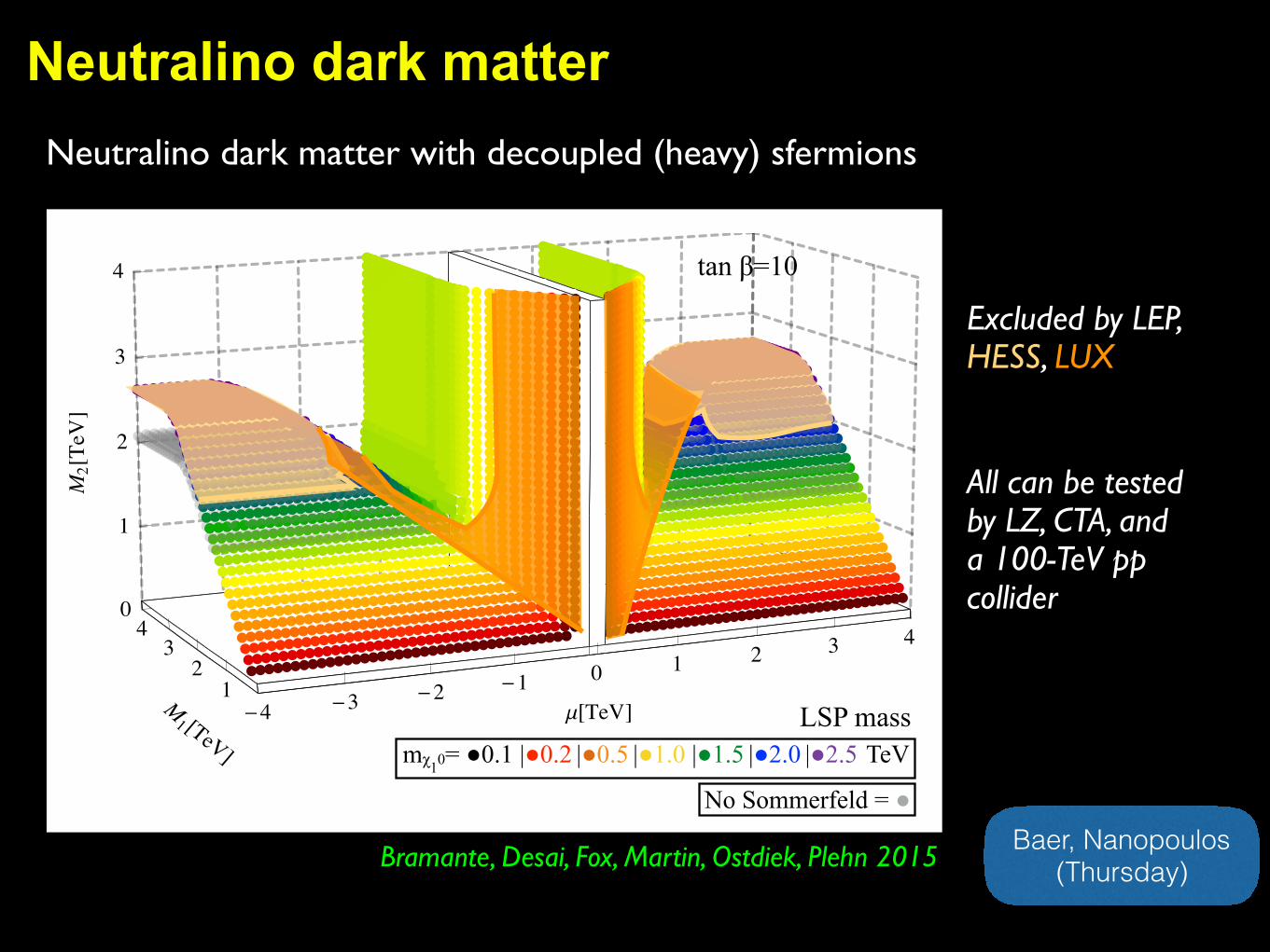
Figure 1. Left panel: Combinations of neutralino mass parameters M1, M2, µ that produce the correct relicabundance, accounting for Sommerfeld-enhancement, along with the LSP mass. The relic surface withoutSommerfeld enhancement is underlain in gray. Regions excluded by LEP are occluded with a white box.Right panel: The wino fraction of the lightest neutralino.

sfermions are also motivated by models of split supersymmetry, where most scalar supersymmetricpartners are decoupled [58–71].

Neutralinos in the MSSM are mixtures of the spin-12

superpartners of the weak gauge bosons,hypercharge gauge bosons, and Higgs bosons. After electroweak symmetry is broken, the neutraland charged states mix to form neutralinos and charginos, respectively. We identify the neutralinosas �̃0

i = Nij(B̃, W̃ 0, H̃0

u, H̃0

d) and the charginos as �̃±i = Vij(W̃±, H̃±). Here B̃, W̃ , H̃0

d , H̃0

u, are thebino, wino, and higgsino fields; Nij and Vij are the neutralino and chargino mixing matrices in thebino-wino basis, such that i and j index mass and gauge respectively [72]. The bino, wino, andhiggsino mass parameters are M

1

, M2

, and µ, and tan � defines the ratio of up- and down-typeHiggs boson vacuum expectation values in the MSSM.

Assuming that all scalar superpartners are heavy, when the universe cools to Trad

< TeV duringradiation dominated expansion, MSSM neutralinos freeze out to a relic abundance determined bytheir rate of annihilation to Standard Model particles. For neutralinos with masses below 1 TeV, itis often su�cient to use tree-level annihilation cross-sections and ignore the initial state exchangeof photons and weak bosons between annihilating neutralinos. On the other hand, the exchange ofgauge bosons between two initial-state particles can substantially alter the annihilation probabilityof neutralinos with masses above 1 TeV. At threshold this higher-order correction can divergelike 1/v, where v is the relative velocity of the two incoming states. For a Yukawa-like potential,mediated for example by a Z-boson, this e↵ect is cut o↵ at v ⇡ mZ/m�̃, leading to large e↵ects fora large ratio of LSP vs weak boson masses. This non-relativistic modification of the potential oftwo incoming states is called the Sommerfeld e↵ect. For freeze-out temperatures below the mass ofelectroweak bosons (T

freeze-out

⌘ m�̃/20 . 0.1 TeV), and thus for lighter LSPs, the contribution ofW± exchange to the e↵ective potential of neutralino pairs is suppressed by factors of e�mW /Trad [56].

To understand when the Sommerfeld enhancement will a↵ect the freeze-out of mixed neutralinos,it is useful to first consider the thermal relic abundance of pure neutralino states. With decoupledscalars, two neutralinos or charginos can either annihilate through an s-channel Z or Higgs boson,or through a t-channel neutralino or chargino. For the lightest neutralinos the relevant couplings

Bramante, Desai, Fox, Martin, Ostdiek, Plehn 2015

Neutralino dark matter with decoupled (heavy) sfermions

Excluded by LEP, HESS, LUX

All can be tested by LZ, CTA, and a 100-TeV pp collider

Baer, Nanopoulos (Thursday)

QCD axions

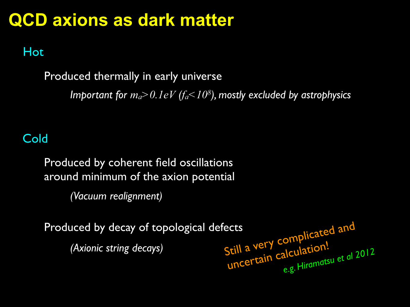
QCD axions as dark matterHot

Cold

Produced thermally in early universe

Important for ma>0.1eV (fa<108), mostly excluded by astrophysics

Produced by coherent field oscillations around minimum of the axion potential

(Vacuum realignment)

Produced by decay of topological defects

(Axionic string decays) Still a very complicated and

uncertain calculation!

e.g. Hiramatsu et al 2012

White Dwarfs Cooling Time

Wa > WcADMX

f a=H Iê2p

Axion IsocurvatureFluctuations

qi=1

qi=0.1

qi=0.01

qi=0.001

qi=0.0001

104 106 108 1010 1012 1014108

1010

1012

1014

1016

1018

10-3

10-6

10-9

10-12

HI @GeVD

f a@Ge

VD

ma@eVD

Expansion rate at end of inflation

PQ s

ymm

etry

bre

akin

g sc

ale

axio

n m

ass

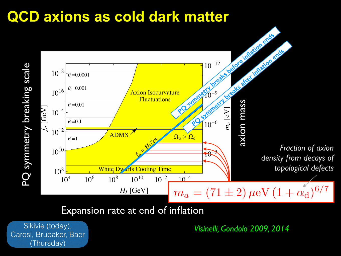
Visinelli, Gondolo 2009, 2014

PQ symmetr

y brea

ks befo

re infl

ation e

nds

PQ symmetr

y brea

ks aft

er infl

ation e

nds

ma = (71± 2)µeV (1 + ↵d)6/7

Fraction of axion density from decays of

topological defects

QCD axions as cold dark matter

Sikivie (today), Carosi, Brubaker, Baer

(Thursday)

Anapole dark matter

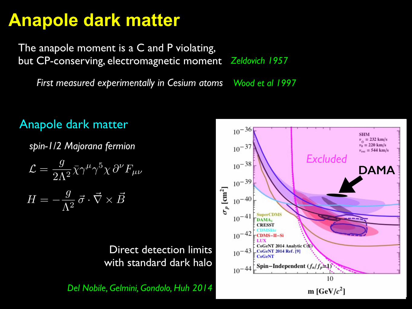
Anapole dark matterThe anapole moment is a C and P violating, but CP-conserving, electromagnetic moment Zeldovich 1957

First measured experimentally in Cesium atoms Wood et al 1997

Anapole dark matter

L =g

2⇤2�̄�µ�5�@⌫Fµ⌫

H = � g

⇤2~� · ~r⇥ ~B

spin-1/2 Majorana fermion

Direct detection limits with standard dark halo

Del Nobile, Gelmini, Gondolo, Huh 2014

ExcludedDAMA

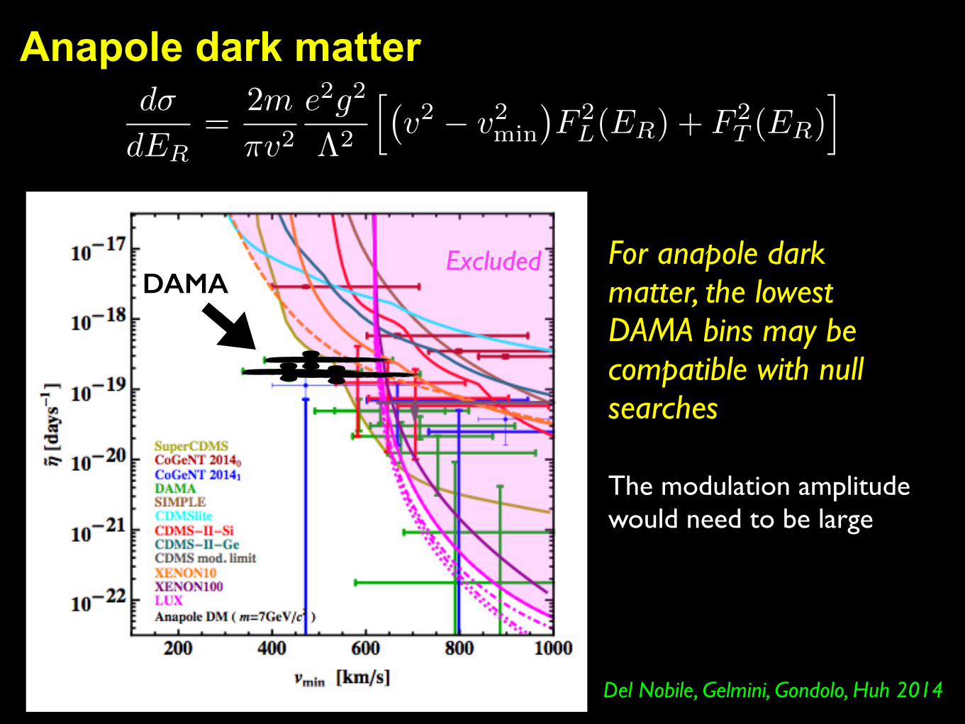
Anapole dark matter

Del Nobile, Gelmini, Gondolo, Huh 2014

For anapole dark matter, the lowest DAMA bins may be compatible with null searches

d�

dER=

2m

⇡v2e2g2

⇤2

h�v2 � v2min

�F 2L(ER) + F 2

T (ER)i

The modulation amplitude would need to be large

ExcludedDAMA

Scalar phantoms

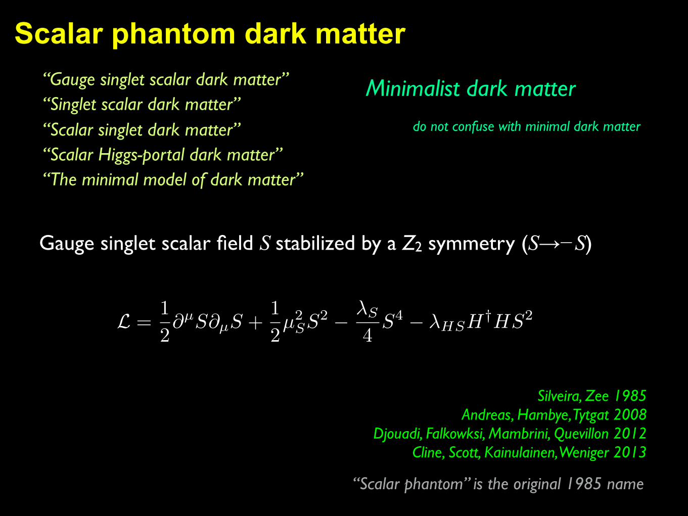
Scalar phantom dark matter

Gauge singlet scalar field S stabilized by a Z2 symmetry (S→−S)

Silveira, Zee 1985Andreas, Hambye, Tytgat 2008

Djouadi, Falkowksi, Mambrini, Quevillon 2012Cline, Scott, Kainulainen, Weniger 2013

do not confuse with minimal dark matter

“Scalar phantom” is the original 1985 name

Minimalist dark matter“Gauge singlet scalar dark matter”“Singlet scalar dark matter”“Scalar singlet dark matter”“Scalar Higgs-portal dark matter”“The minimal model of dark matter”

L =1

2@µS@µS +

1

2µ2SS

2 � �S

4S4 � �HSH

†HS2

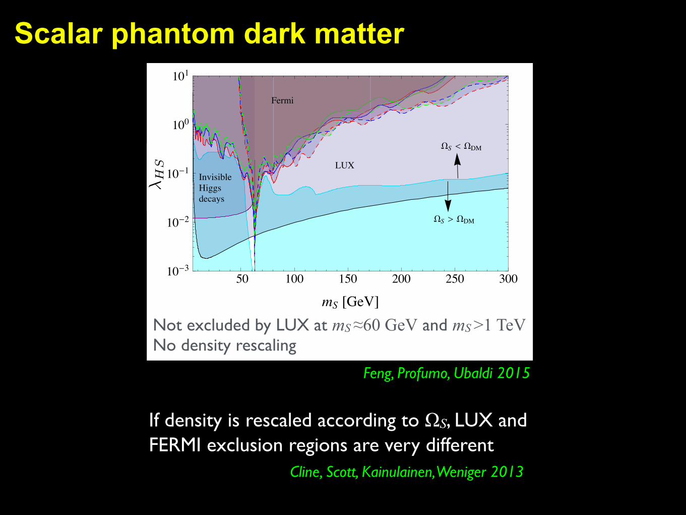
Scalar phantom dark matter

Fermi

InvisibleHiggsdecays

LUX

WS < WDM

WS > WDM

50 100 150 200 250 30010-3

10-2

10-1

100

101

mS @GeVD

a 2

Figure 1. Along the cyan line the real scalar singlet gives the correct dark matter relic abundance.The region below this line corresponds to overabundance and is excluded, while most of the regionabove is excluded by experimental constraints. The strongest limits are from direct detection(LUX [37]): they exclude the region above the black line. Going to masses below a few GeVthe most important constraint comes from invisible Higgs decays searches [40], which exclude theregion above the purple line. We show several lines for the constraints from gamma-ray line searches(Fermi [38]): the plain lines correspond to the annihilation SS ! ��, the dashed lines to SS ! �Z.The colors correspond to di↵erent dark matter density profiles: red is for Einasto, blue for NFW,green for Isothermal. Fermi excludes the area above these lines. The only small region which is notyet excluded is the white area on the lower left part of the plot, close to the resonance mS = mh/2.We zoom into the resonant region in Fig. 2.

where µ2 < 0, � is the quartic coupling for the Higgs, and (�µ2/�)1/2 = v. This potential

is bounded from below, at tree level, provided that �, b4 � 0, and �b4 � a22 for negative a2.

The singlet mass is, at tree level,

m2S = b2 + a2v

2 . (2.3)

The phenomenology of this model is completely determined by the parameters a2 and b2(or mS), since the self-interaction quartic coupling b4 does not play any phenomenologically

observable role (see e.g. [26, 39]).

In this paper we study experimental bounds on the two-dimensional parameter space

{a2,mS} and we update the results of our previous work [26]. Since then, the Higgs has

been discovered [35, 36], thus its mass is no longer a free parameter. In addition, we also

now have constraints on the invisible Higgs decay h ! SS [40–42], and both direct [37]

and indirect [38] detection limits have improved significantly.

– 3 –

Not excluded by LUX at mS ≈60 GeV and mS >1 TeV

�H

S

Feng, Profumo, Ubaldi 2015

No density rescaling

If density is rescaled according to ΩS, LUX and FERMI exclusion regions are very different

Cline, Scott, Kainulainen, Weniger 2013

750-GeV portal

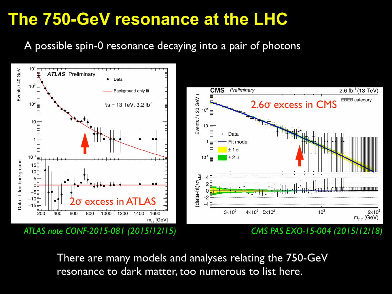
The 750-GeV resonance at the LHC

There are many models and analyses relating the 750-GeV resonance to dark matter, too numerous to list here.

[GeV]γγm200 400 600 800 1000 1200 1400 1600

Even

ts /

40 G

eV

1−10

1

10

210

310

410ATLAS Preliminary

-1 = 13 TeV, 3.2 fbs

Data

Background-only fit

[GeV]γγm200 400 600 800 1000 1200 1400 1600

Dat

a - f

itted

bac

kgro

und

15−10−

5−05

1015

Even

ts /

( 20

GeV

)

-110

1

10

210

DataFit model

σ 1 ±σ 2 ±

EBEB category

(GeV)γ γm210×3 210×4 210×5 310 310×2

stat

σ(d

ata-

fit)/

-4-2024

(13 TeV)-12.6 fbCMS Preliminary

2.6σ excess in CMS

2σ excess in ATLAS

ATLAS note CONF-2015-081 (2015/12/15) CMS PAS EXO-15-004 (2015/12/18)

A possible spin-0 resonance decaying into a pair of photons

750-GeV portal with Majorana dark matter

�� -�

��-�

�

��

��

��

� χ�

��

��

�� χ� = �π

��/Λ = �� -�

��/Λ ≃ �� ⨯ ��-� ��-�

��/Λ = �

��

��

Ω�� = ��

± �σ

Figure 6: DM analysis in the gluon fusion regime. The notation is the same as in Fig. 5.

and we show results for this scenario in Fig. 6. The couplings to gluons for a scalar mediator isresponsible for quite large direct detection rates. As an example, the RG analysis in Section (3.2)yields a direct detection cross section �SI ' c2�S ⇥ 2.2 · 10�46 cm2 for m� = 1TeV and cGG/⇤ '0.03TeV�1. Limits from mono-jet events are not relevant in this DM mass range (see Eq. (40)).The thermal relic line for m� < mS is almost completely excluded by LUX, except for DMmasses extremely close to mS/2. Similar to the photon fusion case, for m� > mS the requiredvalue of c�S suddenly drops and a thermal relic is consistent with LUX bounds. However, theentire parameter space will be deeply probed by LZ. Although the results in Fig. 6 are presentedfor a fixed value of cGG/⇤, it is straightforward to rescale the results. DD bounds scale linearlywith cGG/⇤. This is true also for the the relic line but only for m� < mS, since for larger DMmasses annihilation to mediators dominate and the line is e↵ectively independent on cGG/⇤.

Unlike the photon fusion case discussed above, a thermal relic with pseudo-scalar mediator(right panel of Fig. 6) is less constrained in the gluon fusion regime. Limits from �-ray linessearches are not applicable in this case, since the annihilation cross section in gluons (i.e. theone responsible for a continuum spectrum of photons) is up to 200 times bigger than the one inlines. Fermi limits from �-ray continuum are of course still valid, but they exclude regions wayabove the thermal relic line. As for the scalar case, mono-jet searches do not put bounds inthis DM mass range. In this case, the relic line is very smooth and the drop around m� = mP

is not visible.

5.2 DM Dominated Resonance

The other half of the parameter space corresponds to DM masses below mS/2, yielding the DMdominated resonance scenario discussed in Section 4.3. We use again the output of our LHCstudy to identify interesting classes of DM models.

We now examine the DM phenomenology in the photon fusion regime. Results are shown

20

�� -�

��-�

�

��

��

��

� χ�

��

��

�� χ� = �π

��/Λ = �� -�

��/Λ ≃ �� ⨯ ��-� ��-�

��/Λ = �

��

� ��

Ω�� = �� ± �σ

Figure 6: DM analysis in the gluon fusion regime. The notation is the same as in Fig. 5.

and we show results for this scenario in Fig. 6. The couplings to gluons for a scalar mediator isresponsible for quite large direct detection rates. As an example, the RG analysis in Section (3.2)yields a direct detection cross section �SI ' c2�S ⇥ 2.2 · 10�46 cm2 for m� = 1TeV and cGG/⇤ '0.03TeV�1. Limits from mono-jet events are not relevant in this DM mass range (see Eq. (40)).The thermal relic line for m� < mS is almost completely excluded by LUX, except for DMmasses extremely close to mS/2. Similar to the photon fusion case, for m� > mS the requiredvalue of c�S suddenly drops and a thermal relic is consistent with LUX bounds. However, theentire parameter space will be deeply probed by LZ. Although the results in Fig. 6 are presentedfor a fixed value of cGG/⇤, it is straightforward to rescale the results. DD bounds scale linearlywith cGG/⇤. This is true also for the the relic line but only for m� < mS, since for larger DMmasses annihilation to mediators dominate and the line is e↵ectively independent on cGG/⇤.

Unlike the photon fusion case discussed above, a thermal relic with pseudo-scalar mediator(right panel of Fig. 6) is less constrained in the gluon fusion regime. Limits from �-ray linessearches are not applicable in this case, since the annihilation cross section in gluons (i.e. theone responsible for a continuum spectrum of photons) is up to 200 times bigger than the one inlines. Fermi limits from �-ray continuum are of course still valid, but they exclude regions wayabove the thermal relic line. As for the scalar case, mono-jet searches do not put bounds inthis DM mass range. In this case, the relic line is very smooth and the drop around m� = mP

is not visible.

5.2 DM Dominated Resonance

The other half of the parameter space corresponds to DM masses below mS/2, yielding the DMdominated resonance scenario discussed in Section 4.3. We use again the output of our LHCstudy to identify interesting classes of DM models.

We now examine the DM phenomenology in the photon fusion regime. Results are shown

20

�� -�

��-�

��-�

�

��

��

��

(�χ�

·��)/Λ

��

-�

��

��

�� χ� · ��/Λ = �π ��-�

��⨯��-� ��-�≲ ��/Λ ≲ �� -�

��/Λ = �

�� -�≲ ��/Λ ≲ �� -�

Γ�/�� = �% (��/Λ ≃ �� -�)

Γ�/�� = ��% (��/Λ ≃ �� -�)

��

��

�+�� (�χ� = ��)

Ω�� = �� ± �

σ

Figure 8: Same as Fig. 7 but for the gluon fusion case. The indirect detection constraints inthe right panel are given for cBB/⇤ ' 0.01TeV�1.

the (m�, c�ScBB/⇤) plane of Fig. 7. A thermal relic consistent with �S ' 45GeV then requiresc�S ' 2.42. If resonance e↵ects are negligible, the relic density line is a universal function ofc�ScBB/⇤ and we have explicitly checked that this rescaling invariance works perfectly for lowervalues of c�S. We expect it to break down for large enough c�S, and we estimate the error wecould make with this rescaling by computing self-consistently the relic density line for a thermalrelic with �S ' mS. As can be seen from Figs. 3 and 4, this corresponds to a larger couplingcBB/⇤ ' 0.53TeV, and a thermal relic would then require c�S ' 6.77. The net result on therelic density is a combination of two e↵ects: a large overall coupling in the cross section and abroader width of the mediator. The green bands in the figure show that these combined e↵ectsare rather mild. Given the lack of constraints from DM searches, a scalar portal in the photonfusion regime leads again to a viable DM candidate. To summarize this discussion we presenthere the values of the parameters consistent with a thermal relic and a scalar width of 45 GeV:

m� ' 289GeV , c�S ' 2.42 , cBB/⇤ ' 0.26TeV�1 , cWW = cGG = 0 . (48)

The LHC analysis allows for values of cWW . cBB, but turning on this coupling does not greatlyimpact the obtained DM parameters m� and c�S.

The pseudo-scalar case is shown in the right panel of Fig. 7 with identical conventions. Weagain give the values of the parameters for a thermal relic and a 45 GeV width:

m� ' 227GeV , c�P ' 1.38 , cBB/⇤ ' 0.26TeV�1 , cWW = cGG = 0 . (49)

However, in contrast to the scalar case, ID limits are now quite severe, and the �-ray linebounds completely rule out a thermal relic even for a cored DM profile like the isothermal one.

Finally, in Fig. 8 we consider the gluon fusion regime for a DM dominated resonance. Inboth panels, cBB/⇤ and cGG/⇤ are understood to be within the range written in the label,

22

�� -�

��-�

��-�

�

��

��

��

(�χ�

·��)/Λ

��

-�

��

��

�� χ� · ��/Λ = �π ��-�

��⨯��-� ��-�≲ ��/Λ ≲ �� -�

��/Λ = �

�� -�≲ ��/Λ ≲ �� -�

Γ�/�� = �% (��/Λ ≃ �� -�)

Γ�/�� = ��% (��/Λ ≃ �� -�)

��

�

��

��

�+�� (�χ� = ��)

��Ω��

= �� ± �σ

Figure 8: Same as Fig. 7 but for the gluon fusion case. The indirect detection constraints inthe right panel are given for cBB/⇤ ' 0.01TeV�1.

the (m�, c�ScBB/⇤) plane of Fig. 7. A thermal relic consistent with �S ' 45GeV then requiresc�S ' 2.42. If resonance e↵ects are negligible, the relic density line is a universal function ofc�ScBB/⇤ and we have explicitly checked that this rescaling invariance works perfectly for lowervalues of c�S. We expect it to break down for large enough c�S, and we estimate the error wecould make with this rescaling by computing self-consistently the relic density line for a thermalrelic with �S ' mS. As can be seen from Figs. 3 and 4, this corresponds to a larger couplingcBB/⇤ ' 0.53TeV, and a thermal relic would then require c�S ' 6.77. The net result on therelic density is a combination of two e↵ects: a large overall coupling in the cross section and abroader width of the mediator. The green bands in the figure show that these combined e↵ectsare rather mild. Given the lack of constraints from DM searches, a scalar portal in the photonfusion regime leads again to a viable DM candidate. To summarize this discussion we presenthere the values of the parameters consistent with a thermal relic and a scalar width of 45 GeV:

m� ' 289GeV , c�S ' 2.42 , cBB/⇤ ' 0.26TeV�1 , cWW = cGG = 0 . (48)

The LHC analysis allows for values of cWW . cBB, but turning on this coupling does not greatlyimpact the obtained DM parameters m� and c�S.

The pseudo-scalar case is shown in the right panel of Fig. 7 with identical conventions. Weagain give the values of the parameters for a thermal relic and a 45 GeV width:

m� ' 227GeV , c�P ' 1.38 , cBB/⇤ ' 0.26TeV�1 , cWW = cGG = 0 . (49)

However, in contrast to the scalar case, ID limits are now quite severe, and the �-ray linebounds completely rule out a thermal relic even for a cored DM profile like the isothermal one.

Finally, in Fig. 8 we consider the gluon fusion regime for a DM dominated resonance. Inboth panels, cBB/⇤ and cGG/⇤ are understood to be within the range written in the label,

22

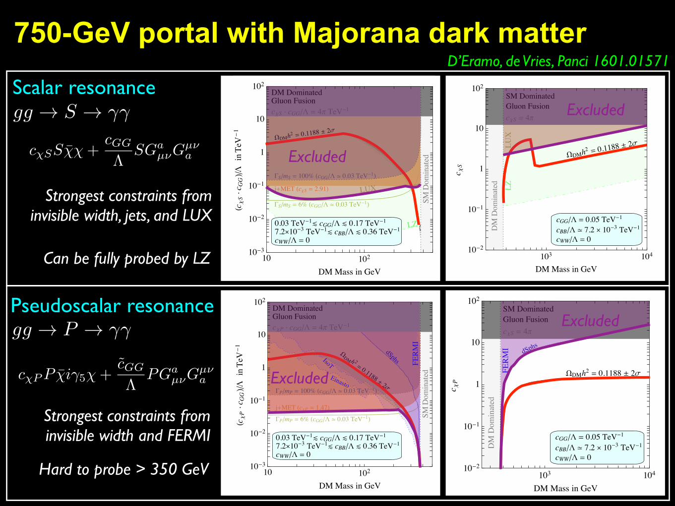
gg ! S ! ��

gg ! P ! ��Pseudoscalar resonance

Scalar resonanceD’Eramo, de Vries, Panci 1601.01571

c�PP �̄i�5�+c̃GG

⇤PGa

µ⌫Gµ⌫a

c�SS�̄�+cGG

⇤SGa

µ⌫Gµ⌫a Excluded

Excluded

Excluded

Excluded

Strongest constraints frominvisible width, jets, and LUX

Can be fully probed by LZ

Strongest constraints frominvisible width and FERMI

Hard to probe > 350 GeV

Self-interacting dark matter

Self-interacting dark matter

Proposed as solution to ‘cusp vs core’ and ‘too big to fail’ puzzles in collisionless dark matter simulations. Spergel, Steinhardt 1999

1 barn/GeV = 0.6 cm2/g

Tested on cluster and galaxy collisionsRandall et al 2008σ/m < 0.7 cm2/g mass loss in Bullet Cluster

Harvey et al 2015σ/m < 0.47 cm2/g 72 cluster collisionsMassey et al 2015σ/m = (1.7±0.7)×10-4 cm2/g in Abell 3827 (?)

Several particle models existLight mediator

Hidden vector dark matter (HVDM)

Feng, Kaplinghat, Yu; Buckley, Fox 2009; Tulin, Yu, Zurek 2013

Hambye 2008

Dark matter is 3 gauge bosons of a hidden SU(2) group spontaneously broken by a hidden Higgs doublet coupled to the SM Higgs. Allowed in some regimes Bernal et al 2015

Yu, Bullock, Boddy (Thursday)

Dynamical dark matter

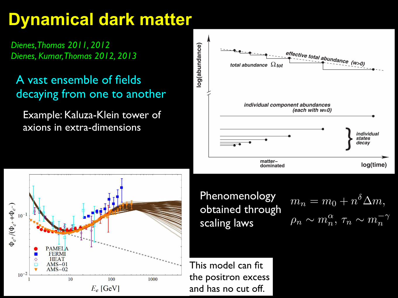
Dynamical dark matterDienes, Thomas 2011, 2012Dienes, Kumar, Thomas 2012, 2013

in all cosmological eras, the presence of an effective weff

which differs (however slightly) from zero would thensignify a departure from the traditional dark-matterscenarios.

We can also understand this at a mathematical level. Thefact that each individual dark-matter component has anabundance which follows the behavior in Eq. (1) with w ¼0 does not guarantee that their sum !tot must follow thesame behavior. Indeed, the two effects which can alter thetime-evolution of the sum !tot in our scenario are a pos-sible staggered turn-on at early times, and the individuallydecaying dark-matter components at late times. Thusthe time-dependence of !tot need not necessarily followEq. (1) with w ¼ 0.

One possibility, of course, is that !tot will continue tofollow Eq. (1), but with some other effective value weff .However, even this outcome requires that our individualdark-matter components exhibit certain relationshipsbetween their abundances and lifetimes which need notactually hold for our dark-matter ensemble. Therefore, ingeneral, we expect that !tot might exhibit a time-dependence which does not resemble that given inEq. (1) for any constant weff . Or, to phrase this somewhatdifferently, we expect that in general, our effectiveequation-of-state parameter weff might itself be time-dependent. We therefore seek to define a function weffðtÞwhich parametrizes a time-dependent equation of state forour dynamical dark-matter ensemble as a whole.

In order to define such an effective functionweffðtÞ, let usfirst recall that the traditional parameterw is fundamentallydefined through the relation p ¼ w! where p and ! are,respectively, the pressure and energy density of the ‘‘fluid’’in question. Of course, in an FRW universe with radius R,the conservation law for energy density dE ¼ $pdV

yields the relation dðR3!Þ ¼ $pdðR3Þ, from which it im-mediately follows that ðpþ !ÞdR3=R3 ¼ $d! or3ðpþ !Þd logR ¼ $d!. Recognizing pþ ! ¼ ð1þ wÞ!and d logR ¼ Hdt where H is the Hubble parameter, wethus have

3Hð1þ wÞ ¼ $d log!

dt: (6)

This is a completely general relation which makes noassumptions about the time-(in)dependence of w. Wemay therefore take this to be our fundamental definitionfor weffðtÞ—i.e.,

weffðtÞ & $!1

3H

d log!tot

dtþ 1

"

¼

8>>><>>>:

$ 12

!d log!tot

d logt

"forRH=MD eras

$ 23

!d log!tot

d logt

"þ 1

3 forRD era.

(7)

Note that while our derivation has thus far been completelygeneral, we have specialized to specific cosmological erasin passing to the final expressions in Eq. (7). Specifically,we have written !tot ¼ !tot!crit and taken 3H ' "=twhere" ¼ 2 (RH=MD), " ¼ 3=2 (RD).The final expressions in Eq. (7) are easy to interpret

physically, since the double-logarithmic derivatives whichappear in these expressions are nothing but the slopes in thesketches in Figs. 1 and 2. However, the important point ofthis derivation has been to demonstrate that weff defined asin Eq. (7) continues to have a direct interpretation as a trueequation-of-state parameter relating energy density andpressure, even when weff is time-dependent. No otherdefinition of weff would have had this property.The results in Eq. (7) provide a relation betweenweff and

!totðtÞ. However, it is also possible to derive a similarrelation between weff and #. Assuming that we restrictour attention to periods of time after all staggered turn-ons are complete (so that the identity of the dark-mattercomponent associated with!0 is fixed), it trivially followsfrom the definition of # in Eq. (5) that

d logð1$ #Þd logt

¼

8><>:

$!d log!tot

d logt

"RH=MD eras

$!d log!tot

d logt

"þ 1

2 RD era:(8)

Using the results in Eq. (7), we therefore find that

weffðtÞ ¼

8>>><>>>:

12

#d logð1$#Þ

d logt

$RH=MD eras

23

#d logð1$#Þ

d logt

$RD era:

(9)

It therefore follows that decreasing # corresponds to posi-tive weff , and vice versa. As a self-consistency check, we

total abundance tot

matter−dominated

individualstatesdecay

individual component abundances(each with w=0)

log(

abun

danc

e)

log(time)

effective total abundance (w>0)

FIG. 2. A sketch of the total dark-matter abundance in ourscenario during the final, matter-dominated era. Even thougheach dark-matter component individually has w ¼ 0, the spec-trum of lifetimes and abundances of these components conspireto produce a time-dependent total dark-matter abundance !tot

which corresponds to an effective equation of state with w> 0.

KEITH R. DIENES AND BROOKS THOMAS PHYSICAL REVIEW D 85, 083523 (2012)

083523-8

A vast ensemble of fields decaying from one to another

Phenomenology obtained through scaling laws

mn = m0 + n��m,

⇢n ⇠ m↵n, ⌧n ⇠ m��

n

11

Significance:1Σ 2Σ 3Σ 4Σ 5Σ

FIG. 2: Contours of the minimum significance level with which a given DDM ensemble is consistent with AMS-02 data,plotted within the (m0,α + γ) DDM parameter space for α = −3 (left panel) and α = −2 (right panel). The coloredregions correspond to DDM ensembles which successfully reproduce the AMS-02 data while simultaneously satisfying all of theapplicable phenomenological constraints outlined in Sect. IV, while the white regions of parameter space correspond to DDMensembles which either cannot simultaneously satisfy these constraints or which fail to match the AMS-02 positron-excess dataat the 5σ significance level or greater. The slight difference between the results shown in the two panels is a consequence ofthe differences in the CMB constraints for the two corresponding values of α.

FIG. 3: Predicted combined fluxes Φe+ +Φ

e− (left panel) and positron fractions Φe+/(Φe

+ +Φe− ) (right panel) corresponding

to the DDM parameter choices lying within those regions of Fig. 2 for which our curves agree with AMS-02 data to within 3σ.These curves are therefore all consistent with current combined-flux data to within 3σ and also consistent with current positron-fraction data to within 3σ (with the color of the curve indicating the precise quality of fit, using the same color scheme inFig. 2). These curves are also consistent with all other applicable phenomenological constraints discussed in Sect. IV. However,despite these constraints, the behavior of the positron-fraction curves beyond E

e± ∼ 350 GeV is entirely unconstrained except

by the internal theoretical structure of the DDM ensemble. Their relatively flat shape in this energy range thus serves as aprediction (and indeed a “smoking gun”) of the DDM framework. Data from AMS-02 [1], HEAT [2], AMS-01 [3], PAMELA [6],FERMI [7, 9], PBB-BETS [45], ATIC [46], and HESS [47] are also shown for reference.

Example: Kaluza-Klein tower of axions in extra-dimensions

This model can fit the positron excess and has no cut off.

Asymmetric dark matter

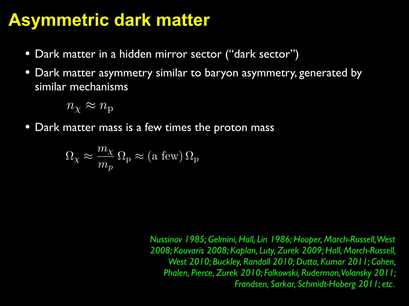
• Dark matter in a hidden mirror sector (“dark sector”)

• Dark matter asymmetry similar to baryon asymmetry, generated by similar mechanisms

• Dark matter mass is a few times the proton mass

Asymmetric dark matter

Nussinov 1985; Gelmini, Hall, Lin 1986; Hooper, March-Russell, West 2008; Kouvaris 2008; Kaplan, Luty, Zurek 2009; Hall, March-Russell,

West 2010; Buckley, Randall 2010; Dutta, Kumar 2011; Cohen, Phalen, Pierce, Zurek 2010; Falkowski, Ruderman, Volansky 2011;

Frandsen, Sarkar, Schmidt-Hoberg 2011; etc.

n� ⇡ np

⌦� ⇡m�

mp⌦p ⇡ (a few) ⌦p

Model-agnostic dark matter

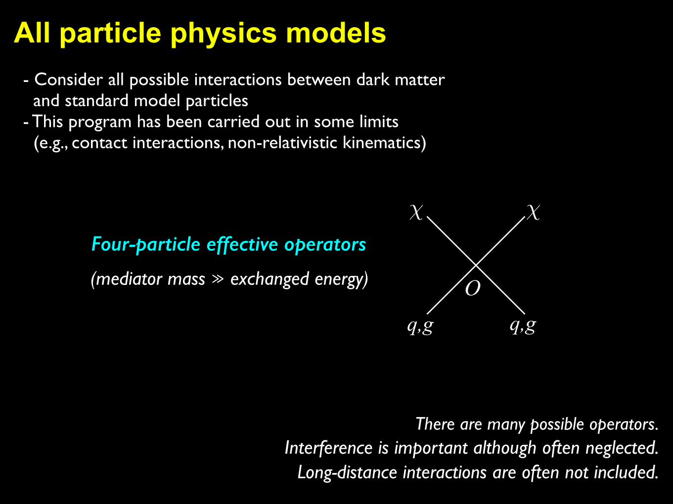
All particle physics models- Consider all possible interactions between dark matter and standard model particles- This program has been carried out in some limits (e.g., contact interactions, non-relativistic kinematics)

χ χ

Oq,g q,g

There are many possible operators.Interference is important although often neglected.

Long-distance interactions are often not included.

Four-particle effective operators

(mediator mass ≫ exchanged energy)

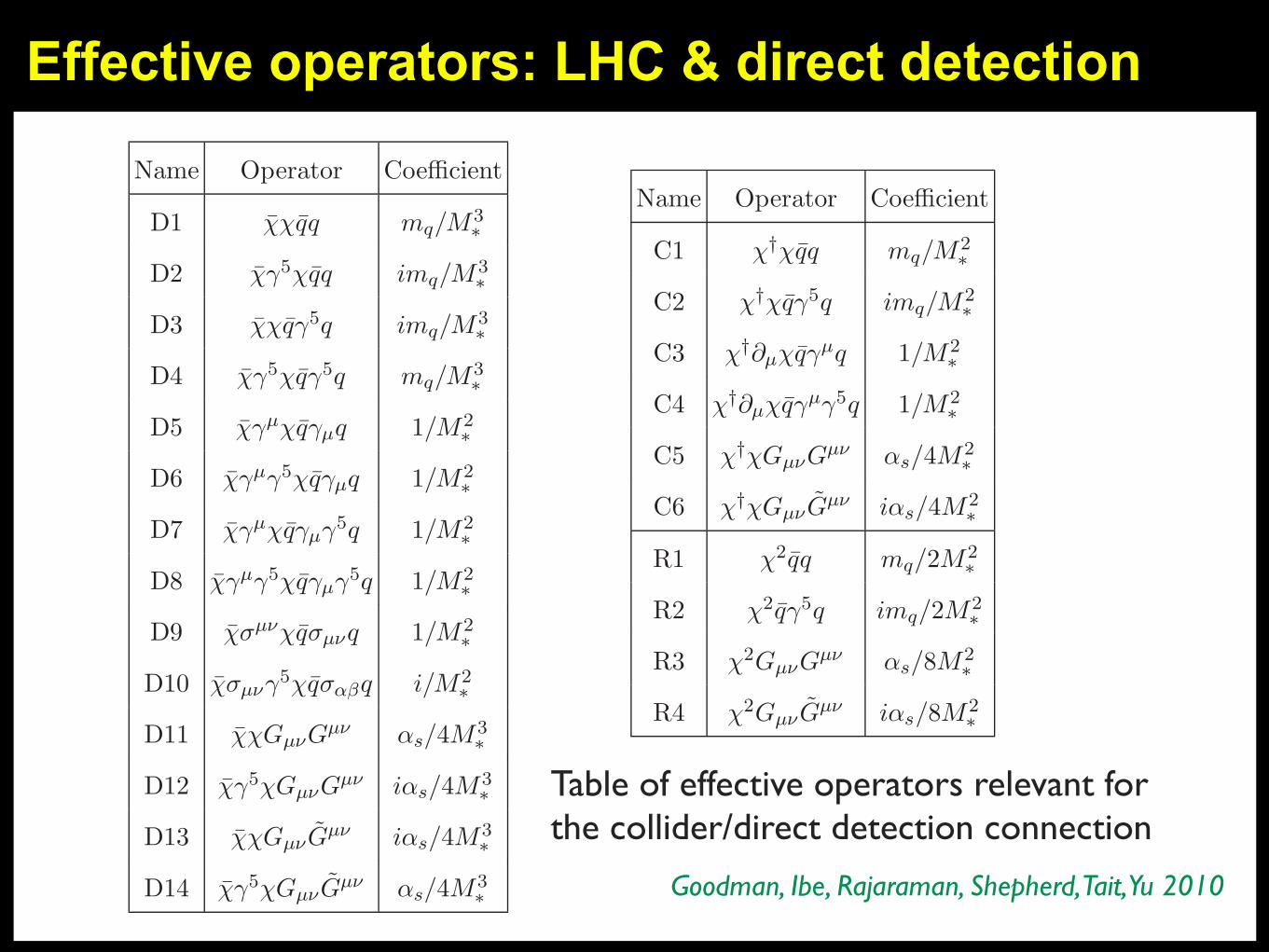
Effective operators: LHC & direct detection

Name Operator Coefficient

D1 χ̄χq̄q mq/M3∗

D2 χ̄γ5χq̄q imq/M3∗

D3 χ̄χq̄γ5q imq/M3∗

D4 χ̄γ5χq̄γ5q mq/M3∗

D5 χ̄γµχq̄γµq 1/M2∗

D6 χ̄γµγ5χq̄γµq 1/M2∗

D7 χ̄γµχq̄γµγ5q 1/M2∗

D8 χ̄γµγ5χq̄γµγ5q 1/M2∗

D9 χ̄σµνχq̄σµνq 1/M2∗

D10 χ̄σµνγ5χq̄σαβq i/M2∗

D11 χ̄χGµνGµν αs/4M3∗

D12 χ̄γ5χGµνGµν iαs/4M3∗

D13 χ̄χGµνG̃µν iαs/4M3∗

D14 χ̄γ5χGµνG̃µν αs/4M3∗

Name Operator Coefficient

C1 χ†χq̄q mq/M2∗

C2 χ†χq̄γ5q imq/M2∗

C3 χ†∂µχq̄γµq 1/M2∗

C4 χ†∂µχq̄γµγ5q 1/M2∗

C5 χ†χGµνGµν αs/4M2∗

C6 χ†χGµνG̃µν iαs/4M2∗

R1 χ2q̄q mq/2M2∗

R2 χ2q̄γ5q imq/2M2∗

R3 χ2GµνGµν αs/8M2∗

R4 χ2GµνG̃µν iαs/8M2∗

TABLE I: Operators coupling WIMPs to SM particles. The operator names beginning with D, C,

R apply to WIMPS that are Dirac fermions, complex scalars or real scalars respectively.

III. COLLIDER CONSTRAINTS

A. Overview

We can constrain M∗ for each operator in the table above by considering the pair pro-

duction of WIMPs at a hadron collider:

pp̄ (pp) → χχ+X. (2)

Since the WIMPs escape undetected, this leads to events with missing transverse energy,

recoiling against additional hadronic radiation present in the reaction.

The most significant Standard Model backgrounds to this process are events where a Z

boson decays into neutrinos, together with the associated production of jets. This back-

ground is irreducible. There are also backgrounds from events where a particle is either

missed or has a mismeasured energy. The most important of these comes from events pro-

7

Table of effective operators relevant for the collider/direct detection connection

Goodman, Ibe, Rajaraman, Shepherd, Tait, Yu 2010

Fox, Harnik, Primulando, Yu 2012

16

CoGeNT

CRESST

CDMS

XENON - 100

DAMAHq ± 33%L

Hc gm cL I q gm qM

monojetrazorcombined

Hc gm cL Ias Gmn GmnM Spin-independent

0.1 1 10 100 100010-46

10-44

10-42

10-40

10-38

10-36

mc@GeVD

sSI@cm

2 D

DAMAHq ± 33%L

PICASSO

XENON 10

COUPP

SIMPLE

monojet

razor

combined

Ic gm g5 cM I q gm g5 qMSpin-dependent

0.1 1 10 100 100010-41

10-39

10-37

10-35

mc@GeVDs

SD@cm

2 D

FIG. 6: Razor limits on spin-independent (LH plot) and spin-dependent (RH plot) DM-nucleon

scattering compared to limits from the direct detection experiments. We also include the mono-

jet limits and the combined razor/monojet limits. We show the constraints on spin-independent

scattering from CDMS [2], CoGeNT [36], CRESST [37], DAMA [38], and XENON-100 [3], and

the constraints on spin-dependent scattering from COUPP [39], DAMA [38], PICASSO [40], SIM-

PLE [41], and XENON-10 [42]. We have assumed large systematic uncertainties on the DAMA

quenching factors: qNa

= 0.3 ± 0.1 for sodium and qI = 0.09 ± 0.03 for iodine [43], which gives

rise to an enlargement of the DAMA allowed regions. All limits are shown at the 90% confidence

level. For DAMA and CoGeNT, we show the 90% and 3� contours based on the fits of [44], and

for CRESST, we show the 1� and 2� contours.

energy required to create a pair of DM is higher.

In addition to the direct detection bounds, we can also convert the collider bounds into a

DM annihilation cross-section, which is relevant to DM relic density calculations and indirect

detection experiments. The annihilation rate is proportional to the quantity h�vreli, where� is the DM annihilation cross section, v

rel

is the relative velocity of the annihilating DM

and h.i is the average over the DM velocity distribution. The quantity �vrel

for OV and OA

operators is 5

�V vrel =1

16⇡⇤4

X

q

s

1� m2

q

m2

�

✓24(2m2

� +m2

q) +8m4

� � 4m2

�m2

q + 5m4

q

m2

� �m2

q

v2rel

◆(14)

�Avrel =1

16⇡⇤4

X

q

s

1� m2

q

m2

�

✓24m2

q +8m4

� � 22m2

�m2

q + 17m4

q

m2

� �m2

q

v2rel

◆(15)

5 A comprehensive study of di↵erent types of operators can be found in Ref. [8].

Spin-independent

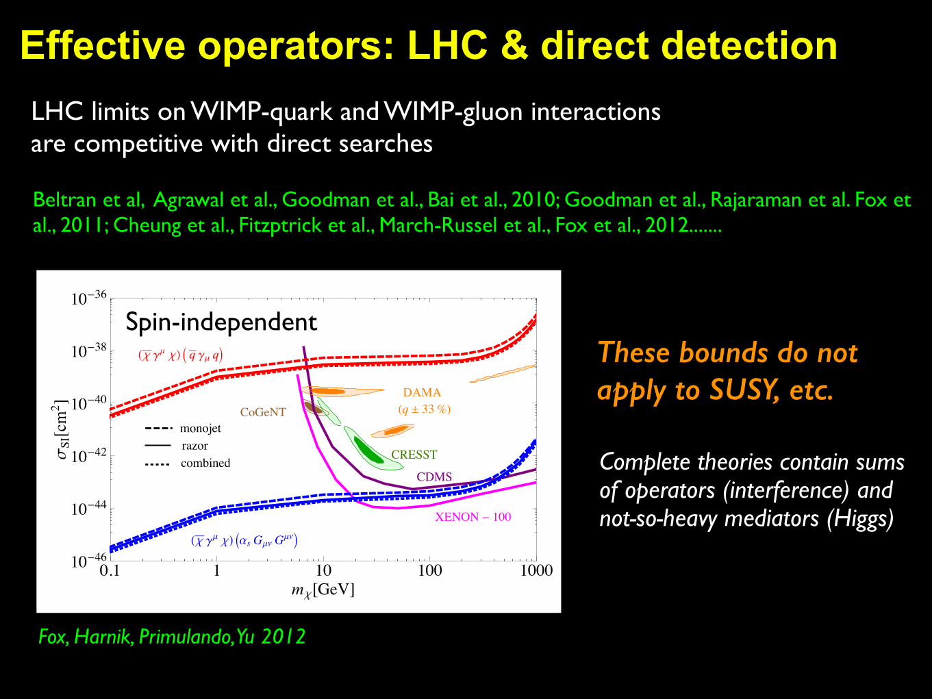
LHC limits on WIMP-quark and WIMP-gluon interactions are competitive with direct searches

Beltran et al, Agrawal et al., Goodman et al., Bai et al., 2010; Goodman et al., Rajaraman et al. Fox et al., 2011; Cheung et al., Fitzptrick et al., March-Russel et al., Fox et al., 2012.......

These bounds do not apply to SUSY, etc.

Complete theories contain sums of operators (interference) and not-so-heavy mediators (Higgs)

Effective operators: LHC & direct detection

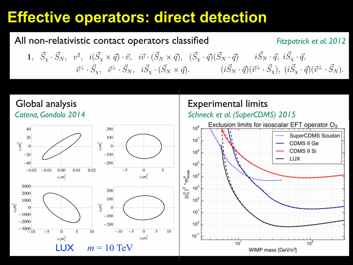
All non-relativistic contact operators classified

of particles of spin one or less (i.e. at most quadratic in either ~S or ~v). In any Lorentz-invariant

local quantum field theory, CP-violation is equivalent to T-violation, so let us first consider

operators that respect time reversal symmetry. These operators are

1, ~S�

· ~SN

, v2, i(~S�

⇥ ~q) · ~v, i~v · (~SN

⇥ ~q), (~S�

· ~q)(~SN

· ~q) (4)

~v? · ~S�

, ~v? · ~SN

, i~S�

· (~SN

⇥ ~q).

The operators in the first line of eq. (4) are parity conserving, while those of the second line

are parity violating. In addition, there are T-violating operators:

i~SN

· ~q, i~S�

· ~q, (5)

(i~SN

· ~q)(~v? · ~S�

), (i~S�

· ~q)(~v? · ~SN

).

In order to determine the interaction of DM particles with the nucleus, the above oper-

ators need to be inserted between nuclear states. Experimentally, the relevant question is

thus what sort of nuclear responses these operators illicit when DM couples to the nucleus.

We find that there are six basic responses corresponding to single-nucleon operators labeled

MJ ;p,n

, ⌃0J ;p,n

, ⌃00J ;p,n

, �J ;p,n

, �̃0J ;pn

, �00J ;p,n

in our discussion of section 3. Five of these re-

sponses (MJ ;p,n

, ⌃0J ;p,n

, ⌃00J ;p,n

, �J ;p,n

, �00J ;p,n

) arise in CP conserving interactions (due to the

exchange of spin one or less), and we therefore primarily focus on this smaller set. Although a

certain CP-violating interaction can be viable (see section 6), finding a UV-model which will

result in the response �̃0J ;pn

seems more challenging. In this paper we provide form factors in

detail for some commonly used elements, however, it is useful to have a heuristic description

for the responses. M is the standard spin-independent response. ⌃0, ⌃00 are the transverse

and longitudinal (with respect to the momentum transfer) components of the nucleon spin

(either p or n). They favor elements with unpaired nucleons. A certain linear combination

of them is the usual spin-dependent coupling. � at zero-momentum transfer measures the

net angular-momentum of a nucleon (either p or n). This response can be an important

contribution to the coupling of DM to elements with unpaired nucleons, occupying an orbital

shell with non-zero angular momentum. Finally, �00, at zero-momentum transfer is related to

(~L · ~S)n,p

. It favors elements with large, not fully occupied, spin-partner angular-momentum

orbitals (i.e. when orbitals j = ` ± 1

2

are not fully occupied). As all these responses view

nuclei di↵erently, a completely model independent treatment of the experiments requires data

to be considered for each response separately (up to interference e↵ects).

Our paper is organized as follows. In section 2, we describe in detail the e↵ective field

theory, emphasizing the non-relativistic building blocks of operators and their symmetry

properties, and demonstrate that the operators in (4,5) describe the most general low-energy

theory given our assumptions. In section 3, we discuss the relevant nuclear physics, and in

particular we thoroughly analyze the possible nuclear response function in a partial wave

basis, which is the standard formalism for such physics. In section 4, we give an overview of

the various new nuclear responses, with an emphasis on their relative strength at di↵erent

elements. In section 5, we summarize these results in a format that can be easily read o↵ and

4

of particles of spin one or less (i.e. at most quadratic in either ~S or ~v). In any Lorentz-invariant

local quantum field theory, CP-violation is equivalent to T-violation, so let us first consider

operators that respect time reversal symmetry. These operators are

1, ~S�

· ~SN

, v2, i(~S�

⇥ ~q) · ~v, i~v · (~SN

⇥ ~q), (~S�

· ~q)(~SN

· ~q) (4)

~v? · ~S�

, ~v? · ~SN

, i~S�

· (~SN

⇥ ~q).

The operators in the first line of eq. (4) are parity conserving, while those of the second line

are parity violating. In addition, there are T-violating operators:

i~SN

· ~q, i~S�

· ~q, (5)

(i~SN

· ~q)(~v? · ~S�

), (i~S�

· ~q)(~v? · ~SN

).

In order to determine the interaction of DM particles with the nucleus, the above oper-

ators need to be inserted between nuclear states. Experimentally, the relevant question is

thus what sort of nuclear responses these operators illicit when DM couples to the nucleus.

We find that there are six basic responses corresponding to single-nucleon operators labeled

MJ ;p,n

, ⌃0J ;p,n

, ⌃00J ;p,n

, �J ;p,n

, �̃0J ;pn

, �00J ;p,n

in our discussion of section 3. Five of these re-

sponses (MJ ;p,n

, ⌃0J ;p,n

, ⌃00J ;p,n

, �J ;p,n

, �00J ;p,n

) arise in CP conserving interactions (due to the

exchange of spin one or less), and we therefore primarily focus on this smaller set. Although a

certain CP-violating interaction can be viable (see section 6), finding a UV-model which will

result in the response �̃0J ;pn

seems more challenging. In this paper we provide form factors in

detail for some commonly used elements, however, it is useful to have a heuristic description

for the responses. M is the standard spin-independent response. ⌃0, ⌃00 are the transverse

and longitudinal (with respect to the momentum transfer) components of the nucleon spin

(either p or n). They favor elements with unpaired nucleons. A certain linear combination

of them is the usual spin-dependent coupling. � at zero-momentum transfer measures the

net angular-momentum of a nucleon (either p or n). This response can be an important

contribution to the coupling of DM to elements with unpaired nucleons, occupying an orbital

shell with non-zero angular momentum. Finally, �00, at zero-momentum transfer is related to

(~L · ~S)n,p

. It favors elements with large, not fully occupied, spin-partner angular-momentum

orbitals (i.e. when orbitals j = ` ± 1

2

are not fully occupied). As all these responses view

nuclei di↵erently, a completely model independent treatment of the experiments requires data

to be considered for each response separately (up to interference e↵ects).

Our paper is organized as follows. In section 2, we describe in detail the e↵ective field

theory, emphasizing the non-relativistic building blocks of operators and their symmetry

properties, and demonstrate that the operators in (4,5) describe the most general low-energy

theory given our assumptions. In section 3, we discuss the relevant nuclear physics, and in

particular we thoroughly analyze the possible nuclear response function in a partial wave

basis, which is the standard formalism for such physics. In section 4, we give an overview of

the various new nuclear responses, with an emphasis on their relative strength at di↵erent

elements. In section 5, we summarize these results in a format that can be easily read o↵ and

4

Effective operators: direct detection

-0.02 -0.01 0.00 0.01 0.02-40

-20

0

20

40

c1mv2

c 3mv2

-5 0 5-200

-100

0

100

200

c4mv2

c 5mv2

-10 -5 0 5 10-200

-100

0

100

200

c8mv2

c 9mv2

-10 -5 0 5 10-3000-2000-1000

0100020003000

c4mv2

c 6mv2

Figure 4. 95% CL profile-likelihood upper limits on the coupling constants c0i (i = 1, 3, . . . , 11) thatcan in principle exhibit correlations, for the LUX experiment and a dark matter particle massm� = 10TeV. There is negligible correlation between c

04 and c

05 and between c

08 and c

09, positive correlation

between c

01 and c

03, and negative correlation between c

04 and c

06.

for a given experiment at a given m� and ⌘ are ellipses in the c0i –c0j plane. These ellipses can

be obtained without random sampling in parameter space by writing

aii(c0i )

2 + 2aijc0i c

0j + ajj(c

0j )

2 = µSconst, (5.4)

where µSconst is the desired value of µS (e.g., its upper limit) and the coe�cients aii, aij ,and ajj are obtained using Eqs. (2.3), (2.5), (4.1), (4.2), and (B.1). The relative size of thesecoe�cients, and thus the shape of the ellipses, is essentially fixed by the nuclear structurefunctions W . The correlation coe�cient rij for the pair of variables c0i and c

0j follows as

rij = � aijpaiiajj

. (5.5)

Fig. 4 shows the ellipses (5.4) for LUX at m� = 10 TeV, with µSconst corresponding to theLUX upper limit. We see that out of the four possible cases, two exhibit negligible correlations(with r45 = �0.027 and r89 = 0.054), one has positive correlation (c01 and c

03 with r13 = 0.90)

and one has negative correlation (c04 and c

06 with r46 = �0.64). These correlations survive

when all experiments are included in the profile likelihood analysis, as seen next.

– 21 –

LUX m = 10 TeV

Catena, Gondolo 2014Global analysis Experimental limits

Schneck et al. (SuperCDMS) 2015

Fitzpatrick et al. 2012

Summary

• There have been many candidates for nonbaryonic dark matter over the years. There seem to be even more now.

• Particle physicists do not lack ideas and are able to escape stronger and stronger experimental constraints.

• The time is ripe for experiments to conclusively find a particle of dark matter.

Dark Matter Particle Candidatesdark matter simulations, which have not been carried out...

Documents

Transcript of Dark Matter Particle Candidatesdark matter simulations, which have not been carried out...