D. Poggi G. G. Katul - Nicholas School of the Environment

Boundary-Layer Meteorol (2010) 136:219–233DOI 10.1007/s10546-010-9503-2

ARTICLE

Evaluation of the Turbulent Kinetic Energy DissipationRate Inside Canopies by Zero- and Level-CrossingDensity Methods

D. Poggi · G. G. Katul

Received: 10 September 2009 / Accepted: 26 April 2010 / Published online: 16 May 2010© Springer Science+Business Media B.V. 2010

Abstract Inferring the vertical variation of the mean turbulent kinetic energy dissipationrate (ε) inside dense canopies remains a basic research problem to be confronted. Usingdetailed laser Doppler anemometry (LDA) measurements collected within a densely arrayedrod canopy, traditional and newly proposed methods to infer ε profiles are compared. Thetraditional methods for estimating ε at a given layer include isotropic relationships applied tothe viscous dissipation scales that are resolved by LDA measurements, higher order structurefunction methods, and residuals of the turbulent kinetic energy budget in which productionand transport terms are all independently inferred. The newly proposed method extends ear-lier approaches based on zero-crossing statistics, which were shown to be promising in anumber of laboratory flows. The extension to account for an arbitrary threshold (hereafterreferred to as the level-crossing method) instead of zero-crossing minimizes the effects ofinstrument noise on the inferred ε. While none of the ε methods employed here can be titledas ‘measured’, these methods differ in their underlying assumptions and simplifications.Above the canopy, where a balance between production and dissipation rate of turbulentkinetic energy is expected, the agreement among all the methods is reasonably good. Inthe lower-to-middle layers of the canopy, all the methods agree except for those based on astructure-function inference of ε. This departure can be attributed to the lack of a well-definedinertial subrange in these layers. In the upper canopy layers, the disagreements between themethods are largest. Even the higher order structure-function methods disagree with eachother when ε is inferred from third- and fifth-order moments. However, for all layers withinthe canopy, the proposed zero- and threshold-crossing methods agree well with estimates of

D. PoggiDipartimento di Idraulica, Trasporti ed Infrastrutture Civili, Politecnico di Torino, Torino, Italy

G. G. Katul (B)Nicholas School of the Environment, Duke University, Box 90328, Durham, NC 27708-0328, USAe-mail: [email protected]

G. G. KatulDepartment of Civil and Environmental Engineering, Pratt School of Engineering, Duke University,Durham, NC 27708, USA

123

220 D. Poggi, G. G. Katul

ε derived from the isotropic relationship applied to the viscous dissipation range. Finally, theadvantages of introducing thresholds to minimize two types of instrument noises, additiveand multiplicative, are briefly discussed.

Keywords Canopy turbulence · Rice’s formula · Telegraphic approximation · Turbulentkinetic energy dissipation rate · Zero-crossing statistics

1 Introduction

Two reviews on the structure of turbulence within the canopy sub-layer (CSL), one publishedabout a decade ago (Finnigan 2000) and another published some three decades ago (Raupachand Thom 1981), virtually share the same message about the difficulty in estimating themean turbulent kinetic energy dissipation rate (ε) inside canopies. A more robust estimationof ε profiles within vegetated canopies is now needed in wide ranging applications such asLagrangian trajectory analysis of passive scalars (Rodean 1996; Poggi et al. 2006) and heavyparticle dispersion (Wilson 2000; Nathan et al. 2002; Katul et al. 2005), relaxation time scaleformulation in higher order closure modeling (Katul et al. 2004; Poggi et al. 2004b; Juanget al. 2008), or in formulating subgrid models for large-eddy simulation (Moeng and Sullivan1994; Sullivan et al. 1994; Patton et al. 1998). There are two reasons why the determinationof ε remains a major research obstacle for canopy flows. Firstly, the work that the mean flowand turbulence exercise against the foliage drag produces turbulent kinetic energy (TKE) bywakes and by spectral short-circuiting of the energy cascade over a broad range of scales, andsecondly the means by which this extra TKE is transferred and dissipated has resisted com-plete theoretical treatments (Finnigan 2000; Poggi and Katul 2006; Cava and Katul 2008).On the experimental side, measuring ε inside canopies remains a formidable challenge, espe-cially using standard sonic anemometry or hot-film probes (Kaimal and Finnigan 1994). Itsindirect inference from structure function scaling laws or as a residual of the TKE budgetcannot be rigorous given that the numerous assumptions employed by these two approachesare routinely violated inside dense canopies. The inference of ε from isotropic relationshipsapplied to the finest length scales commensurate with the Kolmogorov dissipation scale (η)requires the computation of spatial gradients at even smaller spatial scales when comparedto the previous two approaches. These fine-scale measurements are known to be difficult andsensitive to instrumentation filtering and noise contamination even when conducted in themost idealized of flow conditions.

Here, we explore an alternative method to estimate ε within and above canopies, whichwe call the ‘threshold-crossing method’. This approach extends an earlier method that isbased on measuring zero-crossing density and relating this zero-crossing density to the meansquared gradients of the velocity using a number of assumptions (Sreenivasan et al. 1983).The zero-crossing density Nd(0) method (Sreenivasan et al. 1983) employs Rice’s formula(Rice 1945), which states that

Nd(0) =√√√√

q2

4πq2, (1)

where q = dq/dt and q are stationary Gaussian distributed and statistically independent pro-cesses with q = 0, where the overbar indicates time averaging. Shortly after the publicationof Rice’s formula, it was originally suggested that when q represents a longitudinal turbulentvelocity component, ε can be estimated from Nd(0) given its links with the longitudinal

123

Dissipation and Level-Crossing 221

velocity Taylor microscale λ. This linkage is developed and discussed in Sect. 3.2 below.A number of investigations have already shown that ε or the Taylor microscale λ estimatedfrom Nd(0) agree well with independent measurements in several laboratory flows that donot diverge appreciably from Gaussian (Sreenivasan et al. 1983; Kailasnath and Sreenivasan1993). For canopy turbulence applications, the premise that ε may be estimated from Nd(0) israther ‘seductive’ given that, (i) gradient measurements are not required, (ii) no assumptionsare made about scaling laws in the structure functions, and (iii) no simplifications need tobe adopted in the TKE budget for which ε has to be computed as a residual. However, can-opy turbulence is strongly inhomogeneous and non-Gaussian, and hence, the use of Rice’sformula may be highly questionable.

Here, a number of methods to estimate ε profiles inside and above a canopy composedof densely arrayed rods in a flume are compared, where the velocity time series used inthe ε estimation was measured using laser Doppler anemometry. We also extend Rice’sformula to include ‘threshold-crossing’ in lieu of zero-crossing thereby generalizing the zero-crossing approach to any arbitrary threshold. This latter approach minimizes the effects ofnoise on crossing density statistics, which we explore via simulations. A comparison betweenε profiles estimated from higher order structure functions, the residual in TKE budgets wherethe production and transport terms are independently estimated, the isotropic relationshipsapplied to mean squared gradients computed in the viscous dissipation range, Nd(0) andNd(Tc) for various Tc thresholds, is presented.

Throughout, both meteorological and index notation are used with x1 = x , x2 = y andx3 = z representing the longitudinal, lateral, and vertical directions respectively, and withu1 = u, u2 = v, and u3 = w representing the longitudinal, lateral, and vertical velocity com-ponents respectively, with z = 0 being the ground. Primed quantities represent instantaneousturbulent excursions from mean states, the latter being represented by time averaging abovethe canopy, and time and planar averaging inside the canopy (Raupach and Shaw 1982).For notational simplicity, both averaging operators are represented by the overbar, and theroot-mean-squared value of an arbitrary variable q is defined as σq = q ′2.

2 Experimental Set-Up

Much of the experimental set-up is described elsewhere (Poggi et al. 2004a,c,d), but forcompleteness, a brief review is presented. The experiment was conducted in an 18 m long,0.90-m wide, and 1 m deep re-circulating rectangular flume having glass sidewalls to permitoptical access. The canopy was composed of stainless steel cylinders, 120 mm tall (= Hc)

and 4 mm in diameter (= dr ), which were arranged in a regular pattern along a 9-m long testsection. The rod density was 1072 rods m−2 and resulted in a drag coefficient comparableto drag coefficients reported for crops and densely forested canopies (Katul et al. 2004).The stationary flow rate employed here resulted in a friction velocity (= u∗) of 0.098 m s−1

based on the measured shear stress at the canopy top and based on the uniform flow depthHw of 0.60 m. The canopy Reynolds numbers (Re∗ = u∗ Hc/ν) was about 12,000. Theu and w series were collected at 2500–3000 Hz for a sampling duration of 300 s per levelabove the channel bottom using two-component laser Doppler anemometry (LDA). The sam-pling frequency of the LDA was sufficiently high to resolve the entire inertial sub-range andmore than half a decade of the viscous dissipation range above the canopy. Given the planarnon-homogeneity in the single-point statistics within the canopy, as may occur when consid-ering the flow statistics near and away from a rod, 11 planar sampling measurement locationswere employed to compute the spatial average of temporally-averaged flow statistics. These

123


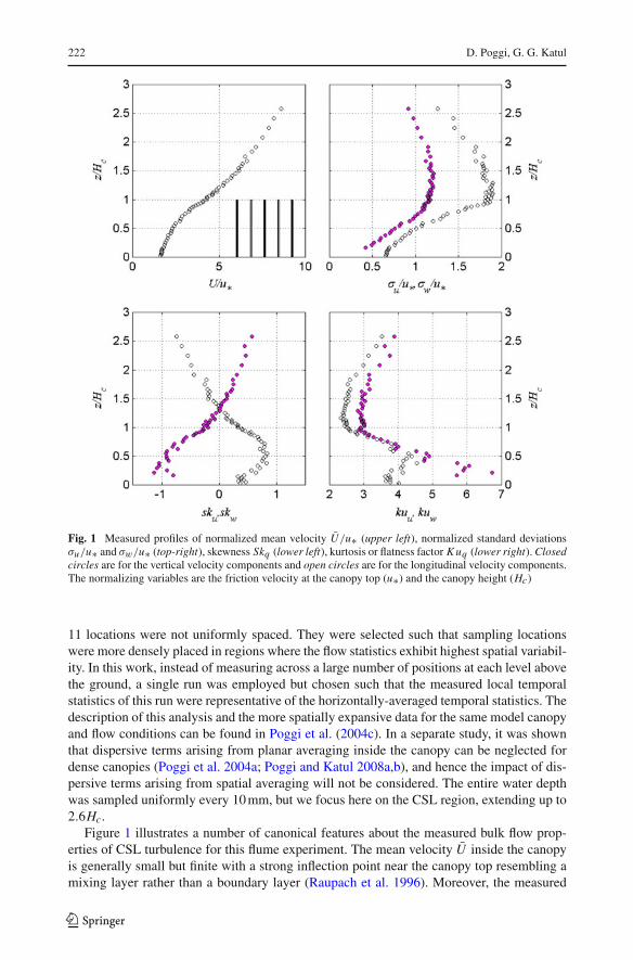
Fig. 1 Measured profiles of normalized mean velocity U/u∗ (upper left), normalized standard deviationsσu/u∗ and σw/u∗ (top-right), skewness Skq (lower left), kurtosis or flatness factor K uq (lower right). Closedcircles are for the vertical velocity components and open circles are for the longitudinal velocity components.The normalizing variables are the friction velocity at the canopy top (u∗) and the canopy height (Hc)

11 locations were not uniformly spaced. They were selected such that sampling locationswere more densely placed in regions where the flow statistics exhibit highest spatial variabil-ity. In this work, instead of measuring across a large number of positions at each level abovethe ground, a single run was employed but chosen such that the measured local temporalstatistics of this run were representative of the horizontally-averaged temporal statistics. Thedescription of this analysis and the more spatially expansive data for the same model canopyand flow conditions can be found in Poggi et al. (2004c). In a separate study, it was shownthat dispersive terms arising from planar averaging inside the canopy can be neglected fordense canopies (Poggi et al. 2004a; Poggi and Katul 2008a,b), and hence the impact of dis-persive terms arising from spatial averaging will not be considered. The entire water depthwas sampled uniformly every 10 mm, but we focus here on the CSL region, extending up to2.6Hc.

Figure 1 illustrates a number of canonical features about the measured bulk flow prop-erties of CSL turbulence for this flume experiment. The mean velocity U inside the canopyis generally small but finite with a strong inflection point near the canopy top resembling amixing layer rather than a boundary layer (Raupach et al. 1996). Moreover, the measured

123


U/u∗ ≈ 3.3 at z/Hc = 1 is consistent with a wide range of field experiments conductedfor dense canopies (Raupach et al. 1996; Katul and Albertson 1998; Finnigan 2000). Thenormalized square root of the longitudinal and vertical velocity variances, σu/u∗ and σw/u∗,are damped inside the canopy though they remain significant even in the vicinity of z = 0.The longitudinal and vertical velocity skewness and flatness factor profiles, computed fromSkq = q ′3/σ 3

q and K uq = q ′4/σ 4q for q = u, w, respectively are also shown. Inside the

canopy, the flow statistics are clearly non-Gaussian, with positively skewed longitudinalvelocity and negatively skewed vertical velocity consistent with arguments that organizedsweeps dominate momentum transfer vis-à-vis ejections (Poggi et al. 2004b; Poggi and Katul2007). Moreover, with intermittency often defined as 3/K uq , it is clear that the flow insidethe canopy is highly intermittent but almost Gaussian close to the canopy top. Hence, fromFig. 1, it is evident that one of the key assumptions for the use of Rice’s formula is violatedfor canopy flows, given the strong departure from Gaussian assumptions in u and w.

3 Methods of Analysis

The various methods used to compute the ε profiles are reviewed next and then comparedagainst this dataset.

3.1 Traditional Methods

The traditional methods for estimating ε include using (1) isotropic relationships for velocitymeasurements that resolve the kinetic energy dissipation rate spectrum, (2) spectra or struc-ture function scaling laws, and (3) the residual of the TKE budget. A brief description of howthe LDA velocity measurements were used for each method is provided next.

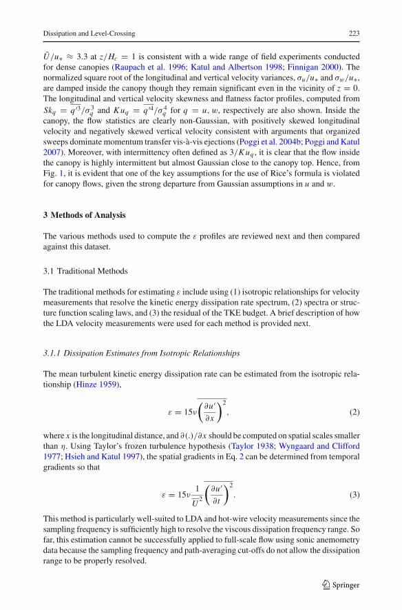
3.1.1 Dissipation Estimates from Isotropic Relationships

The mean turbulent kinetic energy dissipation rate can be estimated from the isotropic rela-tionship (Hinze 1959),

ε = 15ν

(∂u′∂x

)2

, (2)

where x is the longitudinal distance, and ∂(.)/∂x should be computed on spatial scales smallerthan η. Using Taylor’s frozen turbulence hypothesis (Taylor 1938; Wyngaard and Clifford1977; Hsieh and Katul 1997), the spatial gradients in Eq. 2 can be determined from temporalgradients so that

ε = 15ν1

U2

(∂u′∂t

)2

. (3)

This method is particularly well-suited to LDA and hot-wire velocity measurements since thesampling frequency is sufficiently high to resolve the viscous dissipation frequency range. Sofar, this estimation cannot be successfully applied to full-scale flow using sonic anemometrydata because the sampling frequency and path-averaging cut-offs do not allow the dissipationrange to be properly resolved.

123


3.1.2 Structure-Function Approach

The velocity structure functions are widely used to infer ε in atmospheric turbulence (Kaimaland Finnigan 1994). In the case of u, the pth-order structure function velocity difference alongthe longitudinal direction x for separation distance r is given as:

Dp(r) = |[u(x + r) − u(x)]|p. (4)

According to the Kolmogorov’s (1941) second similarity hypothesis (hereafter referred to asK41), Dp(r) in the inertial subrange depends on ε and r only and is given by

Dp(r) = C p (εr)p/3 , (5)

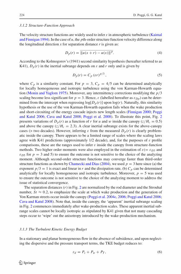
where C p is a similarity constant. For p = 3, C p = 4/5 can be determined analyticallyfor locally homogeneous and isotropic turbulence using the von Karman-Howarth equa-tion (Monin and Yaglom 1975). Moreover, any intermittency corrections modifying the p/3scaling become less significant for p = 3. Hence, ε (labelled hereafter as εDp) can be deter-mined from the intercept when regressing log[Dp(r)] upon log(r). Naturally, this similarityhypothesis or the use of the von Karman-Howarth equation fails when the wake productionand short-circuiting of the energy cascade injects new length scales (Finnigan 2000; Poggiand Katul 2006; Cava and Katul 2008; Poggi et al. 2008). To illustrate this point, Fig. 2presents variations of Dp(r) as a function of r for u and w inside the canopy (z/Hc = 0.5)and above the canopy (z/Hc = 2.3). A clear inertial subrange exists for the above-canopycases (> two decades). However, inferring ε from the measured Dp(r) is clearly problem-atic inside the canopy. There appears to be a limited range of scales where the scaling lawsagree with K41 predictions (approximately 1/2 decade), and, for the purposes of ε profilecomparisons, these are the ranges used to infer ε inside the canopy from structure-functionmethods. Two higher order moments were also employed in the estimation of ε(= εD3 andεD5 for p = 3 and 5) to ensure the outcome is not sensitive to the choice of the analyzingmoment. Although second-order structure functions may converge faster than third-orderstructure functions as shown by Chamecki and Dias (2004), we used p = 3 here since (a) theexponent p/3 = 1 is exact and linear in r and the dissipation rate, (b) C p can be determinedanalytically for locally homogeneous and isotropic turbulence. Moreover, p = 5 was usedto ensure the outcome is not sensitive to the choice of the analyzing moment to address theissue of statistical convergence.

The separation distances (r) in Fig. 2 are normalized by the rod diameter and the Strouhalnumber, St ≈ 0.2, to emphasize the scale at which wake production and the generation ofVon Karman streets occur inside the canopy (Poggi et al. 2004c, 2006; Poggi and Katul 2006;Cava and Katul 2008). Note that, inside the canopy, the ‘apparent’ inertial subrange scalingin Fig. 2 commences immediately after wake-production scales. These apparent inertial sub-range scales cannot be locally isotropic as stipulated by K41 given that not many cascadingsteps occur to ‘wipe’ out the anisotropy introduced by the wake-production mechanism.

3.1.3 The Turbulent Kinetic Energy Budget

In a stationary and planar homogeneous flow in the absence of subsidence, and upon neglect-ing the dispersive and the pressure transport terms, the TKE budget reduces to:

εd = Ps + Pw + PT , (6)

123


Fig. 2 Examples of measured higher order structure functions (D3(r), diamond, and D5(r), circles) for thelongitudinal velocity time series as a function of normalized separation distance r inferred from Taylor’s frozenturbulence hypothesis for four dimensionless distances from the channel bottom (z/Hc). The normalizationof r is based on the rod diameter (dr ) and the dimensionless Strouhal number (St = 0.21) at which wakeproduction occurs. The solid lines show the K41 scaling, the vertical solid lines in the top panels are when rapproaches the size of the von Karman vortices injected in the flow field by the rods

where Ps is the shear production, Pw is the wake production, and PT represents the transportterms. From the observations used herein, we estimated these terms as follows:

Ps = −u′w′ ∂U

∂z, (7a)

Pw = 2CdaU3, (7b)

PT = ∂(w′e′)∂z

, (7c)

with Cd accounting for sheltering effects and local Reynolds number variations with height,and is given elsewhere (Poggi et al. 2004b), a is the frontal area index (Poggi et al. 2004c), e′is the instantaneous turbulent kinetic energy, and e = u′

i u′i/2 is the turbulent kinetic energy.

By estimating Ps, Pw , and PT from the measured profiles of u′w′, U , and w′e′, εd can thenbe computed.

123


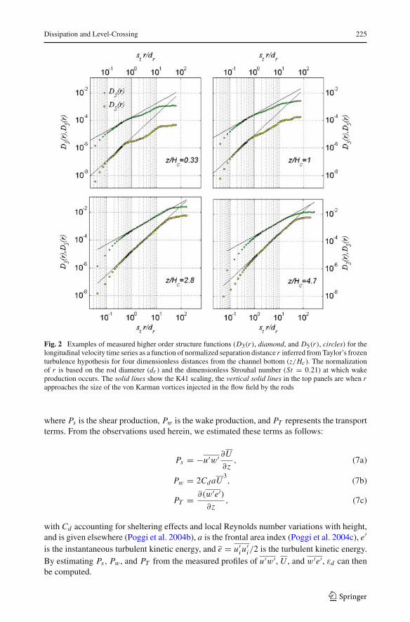
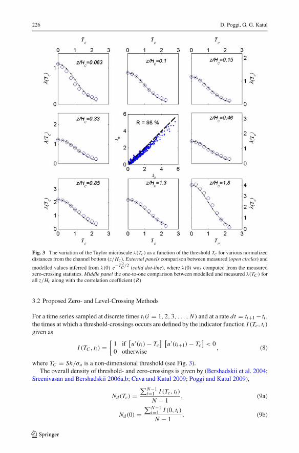
Fig. 3 The variation of the Taylor microscale λ(Tc) as a function of the threshold Tc for various normalizeddistances from the channel bottom (z/Hc). External panels comparison between measured (open circles) and

modelled values inferred from λ(0) e−T 2C /2 (solid dot-line), where λ(0) was computed from the measured

zero-crossing statistics. Middle panel the one-to-one comparison between modelled and measured λ(TC ) forall z/Hc along with the correlation coefficient (R)

3.2 Proposed Zero- and Level-Crossing Methods

For a time series sampled at discrete times ti (i = 1, 2, 3, . . . , N ) and at a rate dt = ti+1 − ti ,the times at which a threshold-crossings occurs are defined by the indicator function I (Tc, ti )given as

I (TC , ti ) ={

1 if[

u′(ti ) − Tc] [

u′(ti+1) − Tc]

< 00 otherwise

, (8)

where TC = Sh/σu is a non-dimensional threshold (see Fig. 3).The overall density of threshold- and zero-crossings is given by (Bershadskii et al. 2004;

Sreenivasan and Bershadskii 2006a,b; Cava and Katul 2009; Poggi and Katul 2009),

Nd(Tc) =∑N−1

i=1 I (Tc, ti )

N − 1, (9a)

Nd(0) =∑N−1

i=1 I (0, ti )

N − 1. (9b)

123


As earlier noted, for a zero mean Gaussian process having a variance σ 2 and an autocor-relation function f (r), the expected number of crossings of a level TC per unit of time isgiven as

Nd(TC ) = 1

π

[− f ′′(0)] 1

2 e(−T 2

C /2)

, (10)

which recovers the zero-crossing formulation when TC = 0, to yield (Sreenivasan et al. 1983):

Nd(0) = 1

π

[− f ′′(0)] 1

2 . (11)

These formulations can be used to estimate ε based on the longitudinal velocity Taylormicroscale. As discussed in Liepmann (1949), the Taylor microscale can be estimate from aparabolic extrapolation of the curvature of f (r) at r = 0, given by (Tennekes and Lumley1972; Pope 2000)

λ =[

−1

2f ′′(0)

]− 12

. (12)

It follows from these expressions that λ can be estimated from threshold- and zero-crossings as

λ(Tc) =√

2

π[Nd(TC )]−1 e

(−T 2C /2

)

, (13a)

λ(0) =√

2

πNd(0)−1. (13b)

Hence, when a threshold Tc is imposed, λ(Tc) = λ(0)e(−T 2

C /2)

. We compared estimates of λ

based on the inferred Nd(Tc) directly from the time series and based on λ(0)e(−T 2

C /2)

, whereonly Nd(0) was inferred from the time series as well. We found that the assumed ‘threshold’correction e

(−T 2C /2

)

to the zero-crossing estimate of λ is quite reasonable for various z/Hc

and Tc values as evident from Fig. 3.To link λ to ε, we note that, for isotropic flow,

(∂u

∂x

)2

= 2σ 2u

λ2 = ε

15ν, (14)

thereby allowing ε to be written as

εTC = 15π2

2ν σ 2

u [Nd(TC )]2 eT 2C , (15)

and

εzc = 15π2

2ν σ 2

u N 2d (0). (16)

The above two formulations have a number of advantages: they are simple to implement andrequire only event-counting, no derivative estimation and no inertial subrange identificationfor structure function computations. What is not known is how robust are these estimates ofε to the assumptions in Rice’s formula inside canopies.

123


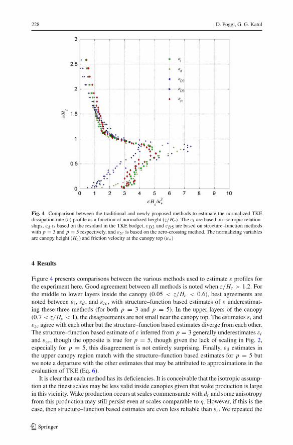
Fig. 4 Comparison between the traditional and newly proposed methods to estimate the normalized TKEdissipation rate (ε) profile as a function of normalized height (z/Hc). The εi are based on isotropic relation-ships, εd is based on the residual in the TKE budget, εD3 and εD5 are based on structure–function methodswith p = 3 and p = 5 respectively, and εzc is based on the zero-crossing method. The normalizing variablesare canopy height (Hc) and friction velocity at the canopy top (u∗)

4 Results

Figure 4 presents comparisons between the various methods used to estimate ε profiles forthe experiment here. Good agreement between all methods is noted when z/Hc > 1.2. Forthe middle to lower layers inside the canopy (0.05 < z/Hc < 0.6), best agreements arenoted between εi , εd , and εzc, with structure–function based estimates of ε underestimat-ing these three methods (for both p = 3 and p = 5). In the upper layers of the canopy(0.7 < z/Hc < 1), the disagreements are not small near the canopy top. The estimates εi andεzc agree with each other but the structure–function based estimates diverge from each other.The structure–function based estimate of ε inferred from p = 3 generally underestimates εi

and εzc, though the opposite is true for p = 5, though given the lack of scaling in Fig. 2,especially for p = 5, this disagreement is not entirely surprising. Finally, εd estimates inthe upper canopy region match with the structure–function based estimates for p = 5 butwe note a departure with the other estimates that may be attributed to approximations in theevaluation of TKE (Eq. 6).

It is clear that each method has its deficiencies. It is conceivable that the isotropic assump-tion at the finest scales may be less valid inside canopies given that wake production is largein this vicinity. Wake production occurs at scales commensurate with dr and some anisotropyfrom this production may still persist even at scales comparable to η. However, if this is thecase, then structure–function based estimates are even less reliable than εi . We repeated the

123


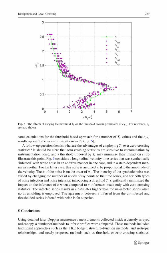
Fig. 5 The effects of varying the threshold Tc on the threshold-crossing estimates of εT C . For reference, εiare also shown

same calculations for the threshold-based approach for a number of Tc values and the εT C

results appear to be robust to variations in Tc (Fig. 5).A follow-up question then is: what are the advantages of employing Tc over zero-crossing

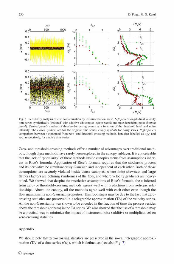
statistics? It should be clear that zero-crossing statistics are sensitive to contamination byinstrumentation noise, and a threshold imposed by Tc may minimize their impact on ε. Toillustrate this point, Fig. 6 considers a longitudinal velocity time series that was synthetically‘infected’ with white noise in an additive manner in one case, and in a state-dependent man-ner in another. For the latter case, this noise is assumed to be proportional to the amplitude ofthe velocity. The σ of the noise is on the order of σu . The intensity of the synthetic noise wasvaried by changing the number of added noisy points to the time series, and for both typesof noise infection and noise intensity, introducing a threshold Tc significantly minimized theimpact on the inference of ε when compared to ε inferences made only with zero-crossingstatistics. The infected series results in ε estimates higher than the un-infected series whenno thresholding is employed. The agreement between ε inferred from the un-infected andthresholded series infected with noise is far superior.

5 Conclusions

Using detailed laser Doppler anemometry measurements collected inside a densely arrayedrod canopy, a number of methods to infer ε profiles were compared. These methods includedtraditional approaches such as the TKE budget, structure–function methods, and isotropicrelationships, and newly proposed methods such as threshold or zero-crossing statistics.

123


Fig. 6 Sensitivity analysis of ε to contamination by instrumentation noise. Left panels longitudinal velocitytime series synthetically ‘infected’ with additive white noise (upper panel) and state dependent-noise (bottompanel). Central panels number of threshold-crossing events as a function of the threshold level and noiseintensity. The closed symbols are for the original time series, empty symbols for noisy series. Right panelscomparison between ε computed from zero- and threshold-crossing methods, hereafter labelled as εZC andεT s , respectively, for a noisy time series

Zero- and threshold-crossing methods offer a number of advantages over traditional meth-ods, though these methods have rarely been explored in the canopy sublayer. It is conceivablethat the lack of ‘popularity’ of these methods inside canopies stems from assumptions inher-ent in Rice’s formula. Application of Rice’s formula requires that the stochastic processand its derivative be simultaneously Gaussian and independent of each other. Both of thoseassumptions are severely violated inside dense canopies, where finite skewness and largeflatness factors are defining syndromes of the flow, and where velocity gradients are heavy-tailed. We showed that despite the restrictive assumptions of Rice’s formula, the ε inferredfrom zero- or threshold-crossing methods agrees well with predictions from isotropic rela-tionships. Above the canopy, all the methods agree well with each other even though theflow maintains its non-Gaussian properties. This robustness may be due to the fact that zero-crossing statistics are preserved in a telegraphic approximation (TA) of the velocity series.All the non-Gaussianity was shown to be encoded in the fraction of time the process residesabove the threshold (or zero) in the TA series. We also showed that the use of a threshold maybe a practical way to minimize the impact of instrument noise (additive or multiplicative) onzero-crossing statistics.

Appendix

We should note that zero-crossing statistics are preserved in the so-call telegraphic approxi-mation (TA) of a time series u′(ti ), which is defined as (see also Fig. 7)

123


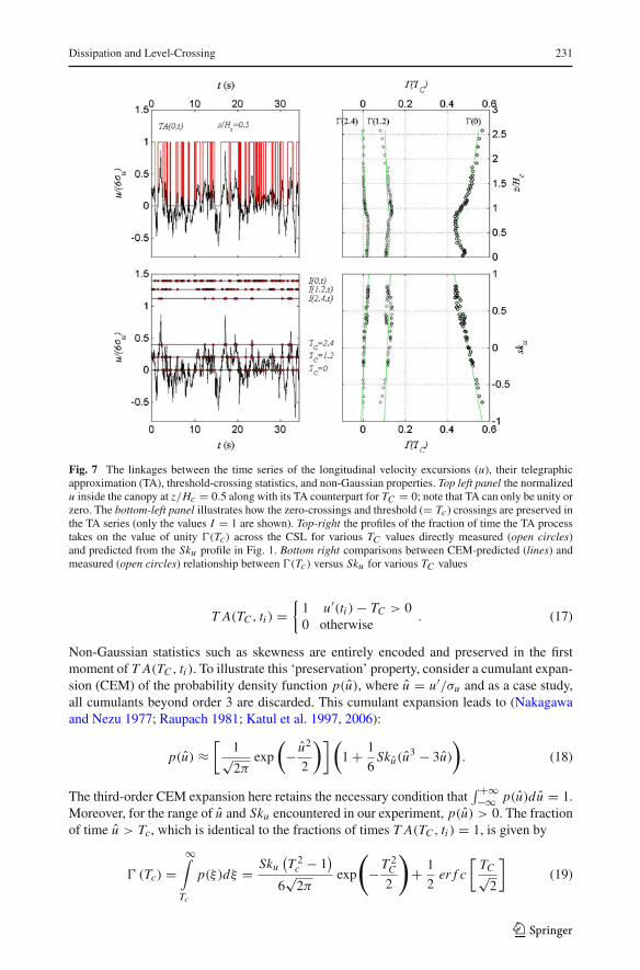
Fig. 7 The linkages between the time series of the longitudinal velocity excursions (u), their telegraphicapproximation (TA), threshold-crossing statistics, and non-Gaussian properties. Top left panel the normalizedu inside the canopy at z/Hc = 0.5 along with its TA counterpart for TC = 0; note that TA can only be unity orzero. The bottom-left panel illustrates how the zero-crossings and threshold (= Tc) crossings are preserved inthe TA series (only the values I = 1 are shown). Top-right the profiles of the fraction of time the TA processtakes on the value of unity (Tc) across the CSL for various TC values directly measured (open circles)and predicted from the Sku profile in Fig. 1. Bottom right comparisons between CEM-predicted (lines) andmeasured (open circles) relationship between (Tc) versus Sku for various TC values

T A(TC , ti ) ={

1 u′(ti ) − TC > 00 otherwise

. (17)

Non-Gaussian statistics such as skewness are entirely encoded and preserved in the firstmoment of T A(TC , ti ). To illustrate this ‘preservation’ property, consider a cumulant expan-sion (CEM) of the probability density function p(u), where u = u′/σu and as a case study,all cumulants beyond order 3 are discarded. This cumulant expansion leads to (Nakagawaand Nezu 1977; Raupach 1981; Katul et al. 1997, 2006):

p(u) ≈[

1√2π

exp

(

− u2

2

)](

1 + 1

6Sku(u3 − 3u)

)

. (18)

The third-order CEM expansion here retains the necessary condition that∫ +∞−∞ p(u)du = 1.

Moreover, for the range of u and Sku encountered in our experiment, p(u) > 0. The fractionof time u > Tc, which is identical to the fractions of times T A(TC , ti ) = 1, is given by

(Tc) =∞∫

Tc

p(ξ)dξ = Sku(

T 2c − 1

)

6√

2πexp

(

− T 2C

2

)

+ 1

2er f c

[TC√

2

]

(19)

123


where er f c [ ] is the complementary error function. Hereafter, we refer to the above expres-sion as the CEM-predicted(Tc)–Sku relationship. The classical zero-crossing (0) is recov-ered upon imposing TC = 0 and results in

(0) =∞∫

0

p(ξ)dξ = 1

2− 1

6√

2πSku . (20)

It is clear from this primitive illustration that a one-to-one connection between the fraction oftime the TA series takes on unity values (a first-moment statistic) and departures from Gaus-sianity (i.e. finite skewness) in the actual velocity time series must exist. Stated differently, (TC ) may capture the non-Gaussian properties embedded in the distributional propertiesof the series. Figure 7 shows that, indeed for the velocity time series, the CEM-predicted (TC )–Sku relationship well reproduces the measurements within and above the canopy andacross a wide range of thresholds. Hence, it is conceivable that N 2

d (TC ) may be less sensitiveto the Gaussian assumptions, given that their effects are already accounted for in (TC ),though this assessment is simply a speculation, and not a rigorous proof.

References

Bershadskii A, Niemela JJ, Praskovsky A, Sreenivasan KR (2004) Clusterization and intermittency of tem-perature fluctuations in turbulent convection. Phys Rev E 69(5):1–5

Cava D, Katul GG (2008) Spectral short-circuiting and wake production within the canopy trunk space of analpine hardwood forest. Boundary-Layer Meteorol 126(3):415–431

Cava D, Katul GG (2009) The effects of thermal stratification on clustering properties of canopy turbulence.Boundary-Layer Meteorol 130(3):307–325

Chamecki M, Dias NL (2004) The local isotropy hypothesis and the turbulent kinetic energy dissipation ratein the atmospheric surface layer. Q J R Meteorol Soc 130:2733–2752

Finnigan J (2000) Turbulence in plant canopies. Ann Rev Fluid Mech 32:519–571Hinze JO (1959) Turbulence. McGraw-Hill, New York, 790 ppHsieh CI, Katul GG (1997) Dissipation methods, Taylor’s hypothesis, and stability correction functions in the

atmospheric surface layer. J Geophys Res Atmos 102(D14):16391–16405Juang JY, Katul GG, Siqueira MB, Stoy PC, McCarthy HR (2008) Investigating a hierarchy of Eulerian closure

models for scalar transfer inside forested canopies. Boundary-Layer Meteorol 128(1):1–32Kailasnath P, Sreenivasan KR (1993) Zero crossings of velocity fluctuations in turbulent boundary layers.

Phys Fluids 5(11):2879–2885Kaimal JC, Finnigan JJ (1994) Atmospheric boundary layer flows: their structure and measurement. Oxford

University Press, New York, 289 ppKatul GG, Albertson JD (1998) An investigation of higher-order closure models for a forested canopy.

Boundary-Layer Meteorol 89(1):47–74Katul G, Hsieh CI, Kuhn G, Ellsworth D, Nie DL (1997) Turbulent eddy motion at the forest–atmosphere

interface. J Geophys Res Atmos 102(D12):13409–13421Katul GG, Mahrt L, Poggi D, Sanz C (2004) One- and two-equation models for canopy turbulence. Boundary-

Layer Meteorol 113(1):81–109Katul GG, Porporato A, Nathan R, Siqueira M, Soons MB, Poggi D, Horn HS, Levin SA (2005) Mechanistic

analytical models for long-distance seed dispersal by wind. Am Nat 166(3):368–381Katul G, Poggi D, Cava D, Finnigan J (2006) The relative importance of ejections and sweeps to momentum

transfer in the atmospheric boundary layer. Boundary-Layer Meteorol 120(3):367–375Liepmann HW (1949) Die anwendung eines satzes uber die nullstellen stochastischer funktionen auf turbu-

lenzmessungen. Helv Phys Acta 22(2):119–126Moeng CH, Sullivan PP (1994) A comparison of shear-driven and buoyancy-driven planetary boundary-layer

flows. J Atmos Sci 51(7):999–1022Monin AS, Yaglom AM (1975) Statistical fluid mechanics. MIT Press, Cambridge, MA, 782 ppNakagawa H, Nezu I (1977) Prediction of contributions to Reynolds Stress from bursting events in open-

channel flows. J Fluid Mech 80:99–128

123


Nathan R, Katul GG, Horn HS, Thomas SM, Oren R, Avissar R, Pacala SW, Levin SA (2002) Mechanismsof long-distance dispersal of seeds by wind. Nature 418(6896):409–413

Patton EG, Shaw RH, Judd MJ, Raupach MR (1998) Large-eddy simulation of windbreak flow. Boundary-Layer Meteorol 87(2):275–306

Poggi D, Katul GG (2006) Two-dimensional scalar spectra in the deeper layers of a dense and uniform modelcanopy. Boundary-Layer Meteorol 121(2):267–281

Poggi D, Katul G (2007) The ejection-sweep cycle over bare and forested gentle hills: a laboratory experiment.Boundary-Layer Meteorol 122(3):493–515

Poggi D, Katul GG (2008a) The effect of canopy roughness density on the constitutive components of thedispersive stresses. Exp Fluids 45(1):111–121

Poggi D, Katul GG (2008b) Micro- and macro-dispersive fluxes in canopy flows. Acta Geophys 56(3):778–799

Poggi D, Katul G (2009) Flume experiments on intermittency and zero-crossing properties of canopy turbu-lence. Phys Fluids 21(6):065103

Poggi D, Katul GG, Albertson JD (2004a) A note on the contribution of dispersive fluxes to momentumtransfer within canopies—research note. Boundary-Layer Meteorol 111(3):615–621

Poggi D, Katul GG, Albertson JD (2004b) Momentum transfer and turbulent kinetic energy budgets within adense model canopy. Boundary-Layer Meteorol 111(3):589–614

Poggi D, Porporato A, Ridolfi L, Albertson JD, Katul GG (2004c) The effect of vegetation density on canopysub-layer turbulence. Boundary-Layer Meteorol 111(3):565–587

Poggi D, Porporato A, Ridolfi L, Albertson JD, Katul GG (2004d) Interaction between large and small scalesin the canopy sublayer. Geophys Res Lett 31(5):4

Poggi D, Katul G, Albertson J (2006) Scalar dispersion within a model canopy: measurements andthree-dimensional Lagrangian models. Adv Water Res 29(2):326–335

Poggi D, Katul GG, Cassiani M (2008) On the anomalous behavior of the Lagrangian structure functionsimilarity constant inside dense canopies. Atmos Environ 42(18):4212–4231

Pope SB (2000) Turbulent flows. Cambidge University Press, UK, 771 ppRaupach MR (1981) Conditional statistics of Reynolds stress in rough-wall and small-wall turbulent boundary

layers. J Fluid Mech 108:363–382Raupach MR, Shaw RH (1982) Averaging procedures for flow within vegetation canopies. Boundary-Layer

Meteorol 22(1):79–90Raupach MR, Thom AS (1981) Turbulence in and above plant canopies. Ann Rev Fluid Mech 13:97–129Raupach MR, Finnigan JJ, Brunet Y (1996) Coherent eddies and turbulence in vegetation canopies: the

mixing-layer analogy. Boundary-Layer Meteorol 78(3–4):351–382Rice SO (1945) Mathematical analysis of random noise. Bell Syst Tech J 24(1):46–156Rodean H (1996) Stochastic Lagrangian models of turbulent diffusion. American Meteorological Society,

Boston, MA, 84 ppSreenivasan KR, Bershadskii A (2006a) Clustering properties in turbulent signals. J Stat Phys 125(5–6):

1145–1157Sreenivasan KR, Bershadskii A (2006b) Finite-Reynolds-number effects in turbulence using logarithmic

expansions. J Fluid Mech 554:477–498Sreenivasan KR, Prabhu A, Narasimha R (1983) Zero-crossings in turbulent signals. J Fluid Mech 137

(DEC):251–272Sullivan PP, McWilliams JC, Moeng CH (1994) A subgrid-scale model for large-eddy simulation of planetary

boundary-layer flows. Boundary-Layer Meteorol 71(3):247–276Taylor GI (1938) The spectrum of turbulence. Proc R Soc Lond A Math Phys Sci 164(A919):0476–0490Tennekes H, Lumley JL (1972) A first course in turbulence. MIT Press, Cambridge, 300 ppWilson JD (2000) Trajectory models for heavy particles in atmospheric turbulence: comparison with obser-

vations. J Appl Meteorol 39(11):1894–1912Wyngaard JC, Clifford SF (1977) Taylor’s hypothesis and high frequency turbulence spectra. J Atmos Sci

34(6):922–929

123

D. Poggi G. G. Katul - Nicholas School of the Environment

Documents

Transcript of D. Poggi G. G. Katul - Nicholas School of the Environment