Curves of Constant Width & Centre Symmetry Sets
46
Curves of Constant Width & Centre Symmetry Sets Andrew David Irving MSc mini-dissertation June 2006 1
Transcript of Curves of Constant Width & Centre Symmetry Sets
Curves of Constant Width & Centre Symmetry Sets
Andrew David Irving
MSc mini-dissertation June 2006
1
Contents
1 Introduction 3
2 Basic Ideas 42.1 Support Function . . . . . . . . . . . . . . . . . . . . . . . . . . . . . 42.2 A Curve of Constant Width . . . . . . . . . . . . . . . . . . . . . . . 52.3 Centre Symmetry Set & Evolute of γ . . . . . . . . . . . . . . . . . . 7
3 Examples of Curves of Constant Width & their CSSs 103.1 Example 1 . . . . . . . . . . . . . . . . . . . . . . . . . . . . . . . . . 103.2 Example 2 . . . . . . . . . . . . . . . . . . . . . . . . . . . . . . . . . 133.3 Example 3 . . . . . . . . . . . . . . . . . . . . . . . . . . . . . . . . . 16
4 Algebraic Expressions 184.1 Example 4 . . . . . . . . . . . . . . . . . . . . . . . . . . . . . . . . . 184.2 Example 5 . . . . . . . . . . . . . . . . . . . . . . . . . . . . . . . . . 194.3 More General Case? . . . . . . . . . . . . . . . . . . . . . . . . . . . 21
5 Barbier’s Theorem 24
6 Morse’s Lemma 276.1 When is h(t1, t2) a Morse function? . . . . . . . . . . . . . . . . . . . 29
7 Reconstruction of a curve from its CSS 327.1 Example 6 . . . . . . . . . . . . . . . . . . . . . . . . . . . . . . . . . 35
8 Maple Appendices 388.1 Appendix 1 . . . . . . . . . . . . . . . . . . . . . . . . . . . . . . . . 388.2 Appendix 2 . . . . . . . . . . . . . . . . . . . . . . . . . . . . . . . . 388.3 Appendix 3 . . . . . . . . . . . . . . . . . . . . . . . . . . . . . . . . 398.4 Appendix 4 . . . . . . . . . . . . . . . . . . . . . . . . . . . . . . . . 398.5 Appendix 5 . . . . . . . . . . . . . . . . . . . . . . . . . . . . . . . . 408.6 Appendix 6 . . . . . . . . . . . . . . . . . . . . . . . . . . . . . . . . 428.7 Appendix 7 . . . . . . . . . . . . . . . . . . . . . . . . . . . . . . . . 43
9 Bibliography 46
2
1 Introduction
This project explores the interesting area of curves of constant width and centre sym-metry sets. Initially one might think that the only curve of constant width would bea circle, but this is in fact not the case as we shall find out. The centre symmetryset of a curve is almost a visual representation of the nature of that curve’s symmetry.
Section 2 outlines the fundamental definitions and concepts, introducing the ideaof defining a curve in terms of its support function, which is central to this project.
In section 3, we look at some examples of curves of constant width and their centresymmetry sets. With many graphical displays, it is hoped that this will make theconcepts outlined in section 2 seem less abstract, improving the understanding ofthe reader.
In section 4, we explore the possibility that parametric examples (some of which
are taken from section 3) could also be expressed algebraically.
Section 5 fills in the gaps for some proofs taken from various literature (all of which
are listed in the Bibliography) and the main theorem prooved here is that of Barbier.
Section 6 looks at Morse’s lemma and Morse functions which can be used for findingparallel tangents to curves (which is very useful for curves of constant width and
centre symmetry sets as we shall see).
Section 7 asks whether it would be possible to start with 2 pieces of curve (say
X and Y ) and find another piece of curve Z such that both X and Z have Y as theircentre symmetry set.
Finally, section 8 features all the Maple programmes I have used in the makingof graphics and lengthly calculations for this project (with annotations).
3
2 Basic Ideas
My main references for this section are [CGI] and [R].
2.1 Support Function
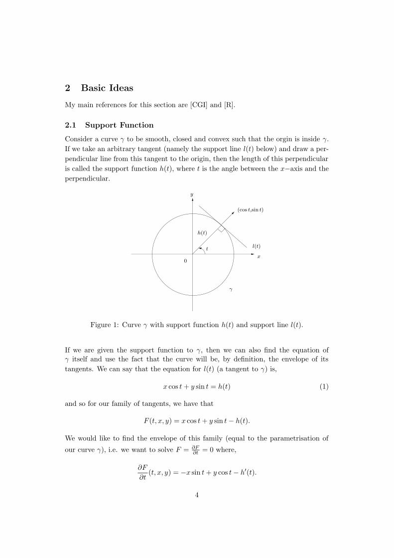
Consider a curve γ to be smooth, closed and convex such that the orgin is inside γ.If we take an arbitrary tangent (namely the support line l(t) below) and draw a per-pendicular line from this tangent to the origin, then the length of this perpendicularis called the support function h(t), where t is the angle between the x−axis and theperpendicular.
t
h(t)
l(t)
(cos t,sin t)
0
γ
x
y
Figure 1: Curve γ with support function h(t) and support line l(t).
If we are given the support function to γ, then we can also find the equation ofγ itself and use the fact that the curve will be, by definition, the envelope of itstangents. We can say that the equation for l(t) (a tangent to γ) is,
x cos t + y sin t = h(t) (1)
and so for our family of tangents, we have that
F (t, x, y) = x cos t + y sin t − h(t).
We would like to find the envelope of this family (equal to the parametrisation of
our curve γ), i.e. we want to solve F = ∂F∂t = 0 where,
∂F
∂t(t, x, y) = −x sin t + y cos t − h′(t).
4
After some calculation, we find the parametrisation of γ to be given by,
x(t) = h(t) cos t − h′(t) sin t (2)
y(t) = h(t) sin t + h′(t) cos t (3)
where ′ denotes a derivative with respect to t (as it will do throughout unless other-
wise stated).
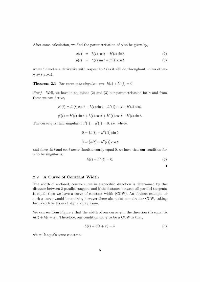
Theorem 2.1 Our curve γ is singular ⇐⇒ h(t) + h′′(t) = 0.
Proof. Well, we have in equations (2) and (3) our parametrisation for γ and fromthese we can derive,
x′(t) = h′(t) cos t − h(t) sin t − h′′(t) sin t − h′(t) cos t
y′(t) = h′(t) sin t + h(t) cos t + h′′(t) cos t − h′(t) sin t.
The curve γ is then singular if x′(t) = y′(t) = 0, i.e. where,
0 =(h(t) + h′′(t)
)sin t
0 =(h(t) + h′′(t)
)cos t
and since sin t and cos t never simultaneously equal 0, we have that our condition forγ to be singular is,
h(t) + h′′(t) = 0. (4)
2.2 A Curve of Constant Width
The width of a closed, convex curve in a specified direction is determined by thedistance between 2 parallel tangents and if the distance between all parallel tangentsis equal, then we have a curve of constant width (CCW). An obvious example ofsuch a curve would be a circle, however there also exist non-circular CCW, takingforms such as those of 20p and 50p coins.
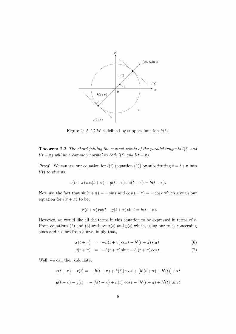
We can see from Figure 2 that the width of our curve γ in the direction t is equal toh(t) + h(t + π). Therefore, our condition for γ to be a CCW is that,
h(t) + h(t + π) = k (5)
where k equals some constant.
5
t
h(t)
l(t)
(cos t,sin t)
0
γ
x
y
l(t+π)
h(t+π)
Figure 2: A CCW γ defined by support function h(t).
Theorem 2.2 The chord joining the contact points of the parallel tangents l(t) and
l(t + π) will be a common normal to both l(t) and l(t + π).
Proof. We can use our equation for l(t) (equation (1)) by substituting t = t+π into
l(t) to give us,
x(t + π) cos(t + π) + y(t + π) sin(t + π) = h(t + π).
Now use the fact that sin(t + π) = − sin t and cos(t + π) = − cos t which give us our
equation for l(t + π) to be,
−x(t + π) cos t − y(t + π) sin t = h(t + π).
However, we would like all the terms in this equation to be expressed in terms of t.From equations (2) and (3) we have x(t) and y(t) which, using our rules concerningsines and cosines from above, imply that,
x(t + π) = −h(t + π) cos t + h′(t + π) sin t (6)
y(t + π) = −h(t + π) sin t − h′(t + π) cos t. (7)
Well, we can then calculate,
x(t + π) − x(t) = − [h(t + π) + h(t)] cos t +[h′(t + π) + h′(t)
]sin t
y(t + π) − y(t) = − [h(t + π) + h(t)] cos t −[h′(t + π) + h′(t)
]sin t
6
which can then be simplified using equation (5) to,
x(t) − x(t + π) = k cos t
y(t) − y(t + π) = k sin t.
Therefore the direction of our chord joining parallel tangents is,
(x(t) − x(t + π), y(t) − y(t + π)) = k (cos t, sin t)
and, with reference to Figure 2 we can see that this is a vector, equal in length anddirection to h(t) + h(t + π) (i.e. itself or any parallel vetor) and by definition, thesupport function is orthogonal to the support line. Therefore parallel tangents to aCCW share a common normal (the chord h(t) + h(t + π) or any parallel).
With this in mind, we would now like to find a parametrisation of the envelope ofparallel tangent chords to a CCW.
2.3 Centre Symmetry Set & Evolute of γ
For now, we will not assume that our curve γ is a CCW (it is however smooth, closed
and convex). Let us find find the envelope of chords joining parallel tangents and,
from above, we know that these chords will join the points (x(t), y(t)) to
(x(t+π), y(t+π)) on γ (see equations (2), (3), (6) and (7)). So the equation of such
a chord (not the vector direction as calculated previously) is given by,
Y − y(t)X − x(t)
=y(t + π) − y(t)x(t + π) − x(t)
where (X, Y ) are coordinates of a chord in R2. From this we can obtain our familyof chords by taking all terms over to one side,
F (t, X, Y ) = [Y − y(t)][x(t + π) − x(t)] − [X − x(t)][y(t + π) − y(t)].
For the envelope of these chords, we need to substitute our known values into F =∂F∂t = 0. From F = 0 we obtain, after some simplification,
Y [(h′ + h′π)s − (h + hπ)c] + X[(hπ + h)s + (h′
π + h′)c] − hh′π + h′hπ = 0.
Finding ∂F∂t and setting it equal to 0 gives,
Y [(h + h′′ + hπ + h′′π)s] + X[(h + h′′ + hπ + h′′
π)c] − hh′′π + h′′hπ = 0
7
and now we can find our envelope of chords. There are some very large expressionsinvolved in this calculation but, with some help from Maple (see Appendix 1), wefind that,
X =−h′hπ sin t + h′′h′
π sin t + hh′π sin t − h′h′′
π sin t + hh′′π cos t − h′′hπ cos t
h + h′′ + hπ + h′′π
Y =−h′hπ cos t + h′′h′
π cos t + hh′π cos t − h′h′′
π cos t + h′′hπ sin t − hh′′π sin t
h + h′′ + hπ + h′′π
(denominator is non-zero, by (4)) yet there is more that we can say about this, con-sider first the centre symmetry set.
DefinitionThe envelope of chords joining parallel tangent points is called the centre symmetryset (CSS).
Proposition 2.1 (X, Y ) is a parametrisation of γ’s CSS.
However, what if γ is a CCW? Well, then we can use the afore mentioned property ofa CCW (equation (5)) and its derivatives in order to express our (X, Y ) in a simplerform, i.e. the following results allow us to find a parametrisation for the CSS on aCCW:
h(t + π) = k − h(t) (8)
h′(t + π) = −h′(t) (9)
h′′(t + π) = −h′′(t). (10)
Again, these calculations are very complicated, so using Maple (see Appendix 2) wefind that the CSS for a CCW can be parametrised by,
(X∗, Y ∗) = (−h′(t) sin t − h′′(t) cos t, h′(t) cos t − h′′(t) sin t)
but this is a a special case.
When γ is a CCW, our chords are common normals to the tangents at points(x(t), y(t)) and (x(t + π), y(t + π)) on γ. From this we can conclude that the enve-lope of chords joining parallel tangent points is equal to the envelope of γ’s normals.Hence (X∗, Y ∗) is a parametrisation of γ’s evolute.
(Note that for the CSS, we only need values of t between 0 and π since takingvalues of t between π and 2π will cover the common normals twice, i.e. if we observethe envelope of chords for t ∈ [0, 2π), then we will see a double cover of the CSS.
Therefore the evolute of γ is equal to the double cover of the CSS).
8
Proposition 2.2 (X∗, Y ∗) is the parametrisation of both the CSS and the evoluteof a CCW.
It seems only appropriate that we should also find the evolute of γ when it is notnecessarily a CCW. The family of normals to γ can be represented by,
G(t, A, B) = (A − x(t)) sin t − (B − y(t)) cos t
and differentiating this with respect to t gives us,
∂G
∂t(t, A, B) =
(h′′ sin t + B − h′ cos t
)sin t +
(A + h′ sin t + h′′ cos t
)cos t.
Solving G = ∂G∂t = 0 gives us,
(A, B) = (−h′(t) sin t − h′′(t) cos t, h′(t) cos t − h′′(t) sin t)
where (A, B) is a parametrisation of γ’s evolute and notice that this is identical to
(X∗, Y ∗) above, where γ was of constant width!
Proposition 2.3 The evolute of a smooth, convex curve with support function h(t)
can be parametrised by (X∗, Y ∗).
Theorem 2.3 Points (X∗, Y ∗) are singular ⇐⇒ h′(t) + h′′′(t) = 0.
Proof. By defintion these points are singular if ddt (X∗) = d
dt (Y ∗) = 0 where,
d
dt(X∗) = −h′′(t) sin t − h′(t) cos t − h′′′(t) cos t + h′′(t) sin t
d
dt(Y ∗) = −h′′′(t) sin t − h′′(t) cos t − h′′(t) cos t − h′(t) sin t
and its easy to see that by cancelling terms and taking out a common factor that,
(d
dt(X∗) ,
d
dt(Y ∗)
)
= −(h′(t) + h′′′(t)
)(cos t, sin t).
Well, since sin t and cos t never equal 0 simultaneously, we have that the conditionfor singular points on the CSS and evolute to our CCW or the evolute of any smooth,convex curve with support function h(t) is that,
h′(t) + h′′′(t) = 0.
9
3 Examples of Curves of Constant Width & their CSSs
3.1 Example 1
In considering an example of a curve of constant width, we said that we requirethe support function h(t) to satisfy the condition h(t) + h(t + π) = k where k is aconstant, an example of which is,
h(t) = a cos2(
3t
2
)
+ b.
This can also be expressed in the form,
h(t) =a
2cos 3t +
a
2+ b
using the trigonometric identity cos 2A = 2 cos2 A − 1. Substituting this into ourparametrisation of γ gives us a CCW with parametric equations,
x =(a
2cos 3t +
a
2+ b)
cos t +3a
2sin 3t sin t
y =(a
2cos 3t +
a
2+ b)
sin t −3a
2sin 3t cos t.
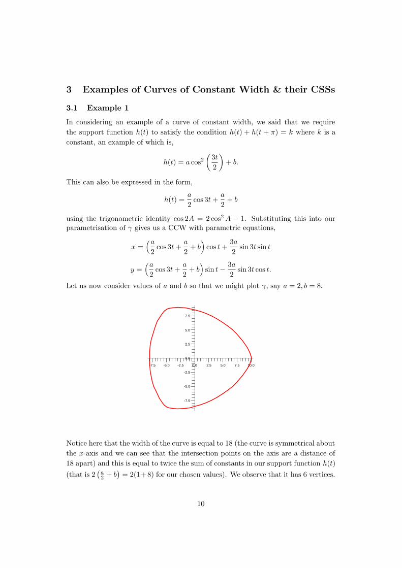
Let us now consider values of a and b so that we might plot γ, say a = 2, b = 8.
10.05.0
5.0
7.5
7.5
0.0
-5.0
2.5
2.5
0.0
-2.5
-7.5
-2.5-5.0-7.5
Notice here that the width of the curve is equal to 18 (the curve is symmetrical aboutthe x-axis and we can see that the intersection points on the axis are a distance of18 apart) and this is equal to twice the sum of constants in our support function h(t)
(that is 2(
a2 + b
)= 2(1+8) for our chosen values). We observe that it has 6 vertices.
10
Theorem 3.1 The CCW with support function of the form h(t) = (∑
Pi cos Qit) +R, where P > 0 and R are constants and Q is some odd integer, is symmetricalabout the horizontal axis.
Proof. For h(t) as defined, our CCW would have parameters,
x(t) =[(∑
Pi cos Qit)
+ R]cos t −
(−∑
PiQi sin Qit)
sin t
y(t) =[(∑
Pi cos Qit)
+ R]sin t +
(−∑
PiQi sin Qit)
cos t
here substituting our h(t) into equations (2) and (3) and expanding our brackets itfollows that,
x(t) =∑
Pi cos Qit cos t + R cos t +∑
PiQi sin Qit sin t
y(t) =∑
Pi cos Qit sin t + R sin t −∑
PiQi sin Qit cos t
are the points on our CCW above the horizontal axis (assume t > 0). Now let t = −t
(such that we are observing points below the horizontal axis) in these equations, then
x(−t) =∑
Pi cos Qit cos t + R cos t +∑
PiQi sin Qit sin t
y(−t) = −∑
Pi cos Qit sin t − R sin t +∑
PiQi sin Qit cos t
using cos(−t) = cos t and sin(−t) = sin t we can concude that x(−t) = x(t) whereas
y(−t) = y(t) so our CCW is symmetrical about the horizontal axis.
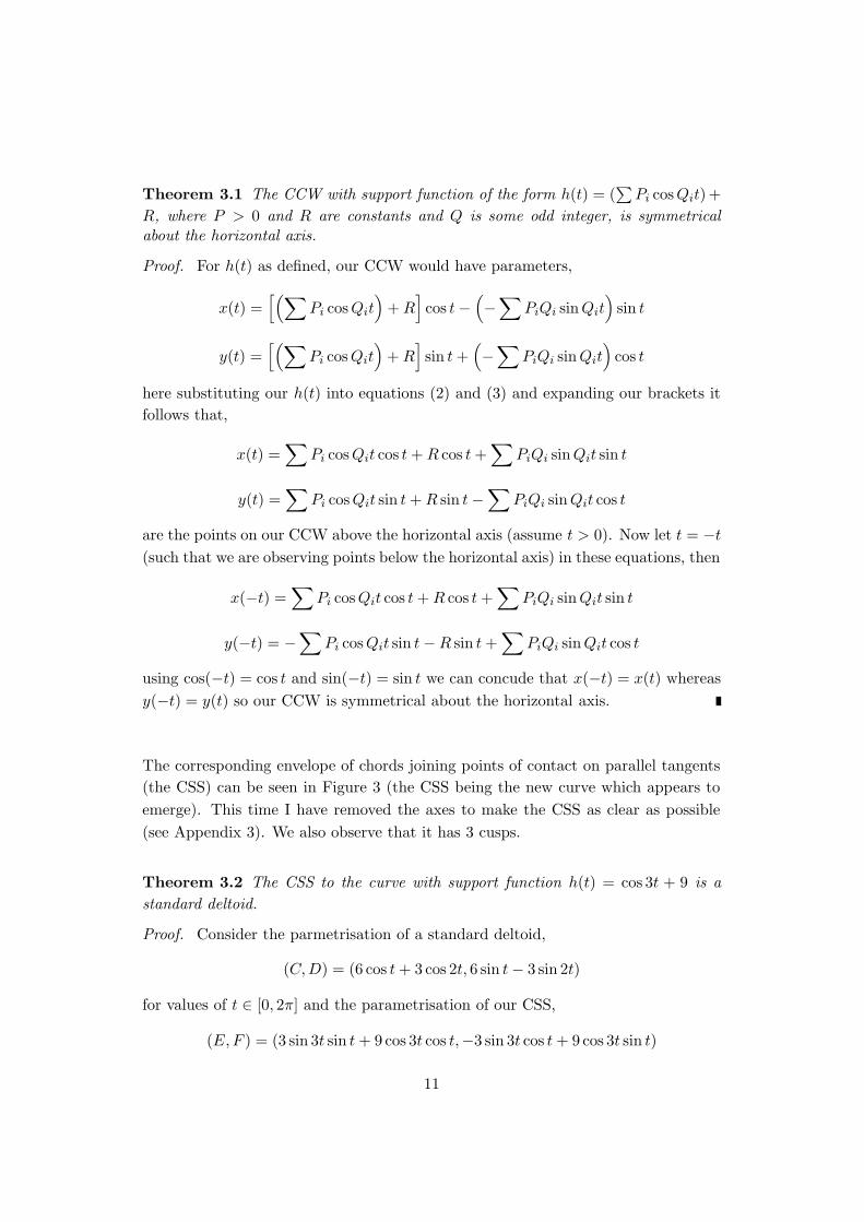
The corresponding envelope of chords joining points of contact on parallel tangents(the CSS) can be seen in Figure 3 (the CSS being the new curve which appears to
emerge). This time I have removed the axes to make the CSS as clear as possible
(see Appendix 3). We also observe that it has 3 cusps.
Theorem 3.2 The CSS to the curve with support function h(t) = cos 3t + 9 is astandard deltoid.
Proof. Consider the parmetrisation of a standard deltoid,
(C, D) = (6 cos t + 3 cos 2t, 6 sin t − 3 sin 2t)
for values of t ∈ [0, 2π] and the parametrisation of our CSS,
(E, F ) = (3 sin 3t sin t + 9 cos 3t cos t,−3 sin 3t cos t + 9 cos 3t sin t)
11
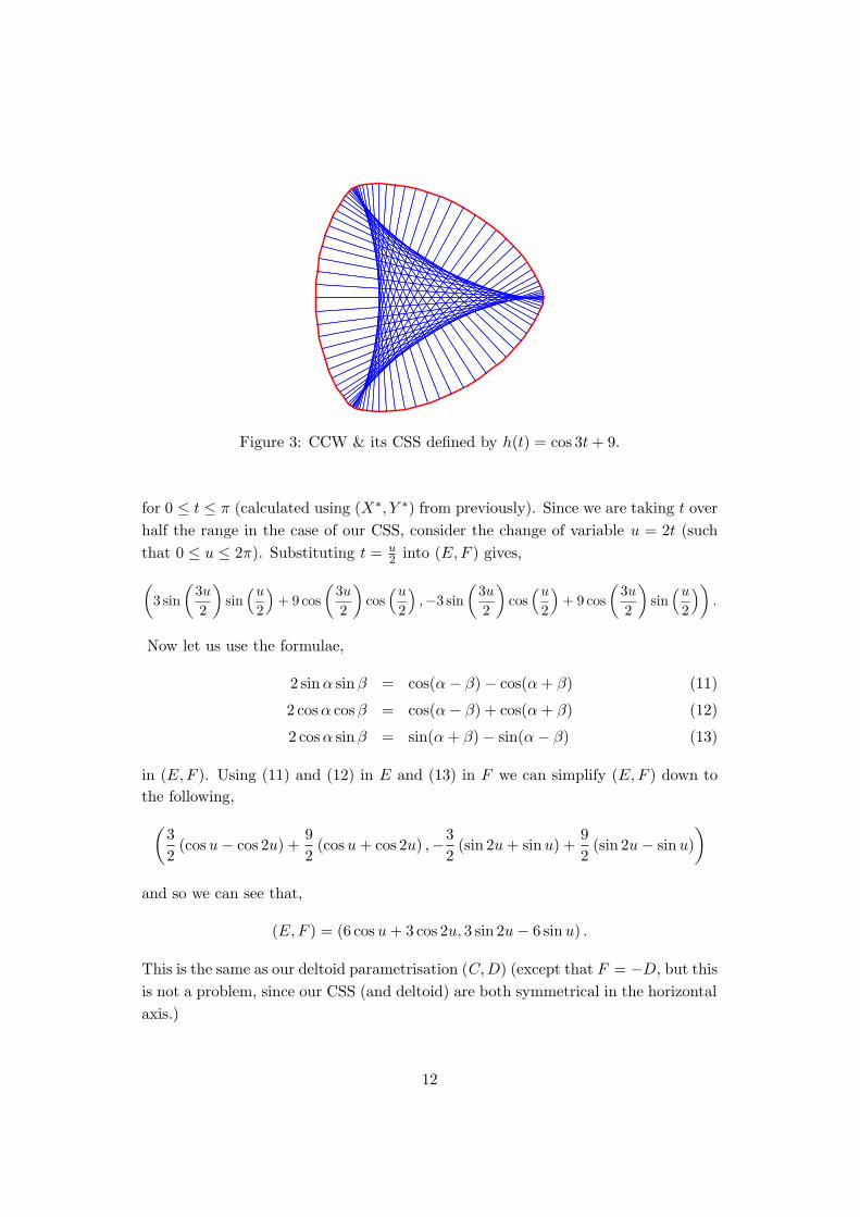
Figure 3: CCW & its CSS defined by h(t) = cos 3t + 9.
for 0 ≤ t ≤ π (calculated using (X∗, Y ∗) from previously). Since we are taking t over
half the range in the case of our CSS, consider the change of variable u = 2t (such
that 0 ≤ u ≤ 2π). Substituting t = u2 into (E, F ) gives,
(
3 sin
(3u
2
)
sin(u
2
)+ 9 cos
(3u
2
)
cos(u
2
),−3 sin
(3u
2
)
cos(u
2
)+ 9 cos
(3u
2
)
sin(u
2
))
.
Now let us use the formulae,
2 sin α sin β = cos(α − β) − cos(α + β) (11)
2 cos α cos β = cos(α − β) + cos(α + β) (12)
2 cos α sin β = sin(α + β) − sin(α − β) (13)
in (E, F ). Using (11) and (12) in E and (13) in F we can simplify (E, F ) down tothe following,
(32
(cos u − cos 2u) +92
(cos u + cos 2u) ,−32
(sin 2u + sin u) +92
(sin 2u − sin u)
)
and so we can see that,
(E, F ) = (6 cos u + 3 cos 2u, 3 sin 2u − 6 sin u) .
This is the same as our deltoid parametrisation (C, D) (except that F = −D, but this
is not a problem, since our CSS (and deltoid) are both symmetrical in the horizontal
axis.)
12

3.2 Example 2
Another example of a support function satisfying our condition for a curve of CCWwould be,
h(t) = a cos2(
5t
2
)
+ b.
This can also be expressed as,
h(t) =a
2cos 5t +
a
2+ b
and so perhaps it becomes clear that any support function of the form h(t) =P cos Qt + R where Q is an odd integer ≥ 3 will give a non-circular CCW, butit is natural to ask why this is the case.
Well, Q has to be odd because, if Q were even then h(t) + h(t + π) 6= k, where
k is a constant, i.e. we would not have a CCW. Also, Q must be ≥ 3 (not 1) sinceif Q were 1, then γ would be a circle.
Substituting h(t) into our parametrisation of γ (equations (2) and (3)), gives usthe parametric equations,
x =(a
2cos 5t +
a
2+ b)
cos t +5a
2sin 5t sin t
y =(a
2cos 5t +
a
2+ b)
sin t −5a
2sin 5t cos t.
Consider values of a and b so that we might plot γ, say for a = 1 and b = 15,
15
10
0
5
-10
15
5
10
-5
-15
0-5-10-15
13
noticing that the width is 31 and it has 10 vertices. The corresponding CSS canbe seen in Figure 4 and it has 5 cusps. So it would appear that a smooth curve γ
with support function h(t) = P cos Qt + R has width 2R, 2Q vertices and the CSShas Q cusps.
Figure 4: CCW & its CSS defined by h(t) = 12 cos 5t + 31
2 .
Theorem 3.3 A CCW with support function of the form h(t) = (∑
Pi cos Qit)+R,where P > 0 and R are constants and Q is some odd integer, has width w = 2R
Proof. The width of our CCW is, by definition,
w = h(t) + h(t + π)
from previously. Well substituting in our h(t) and h(t + π) this becomes,
w =(∑
Pi cos Qit)
+ R +(∑
Pi cos Qi(t + π))
+ R
but we know that cos(t + π) = − cos t so in fact,
w =(∑
P cos Qit)
+ R −(∑
Pi cos Qit)
+ R = 2R
Theorem 3.4 A smooth CCW with support function of the form h(t) = P cos Qt +R, where P > 0 and R are constants and Q is an odd integer ≥ 3, has 2Q vertices.
14
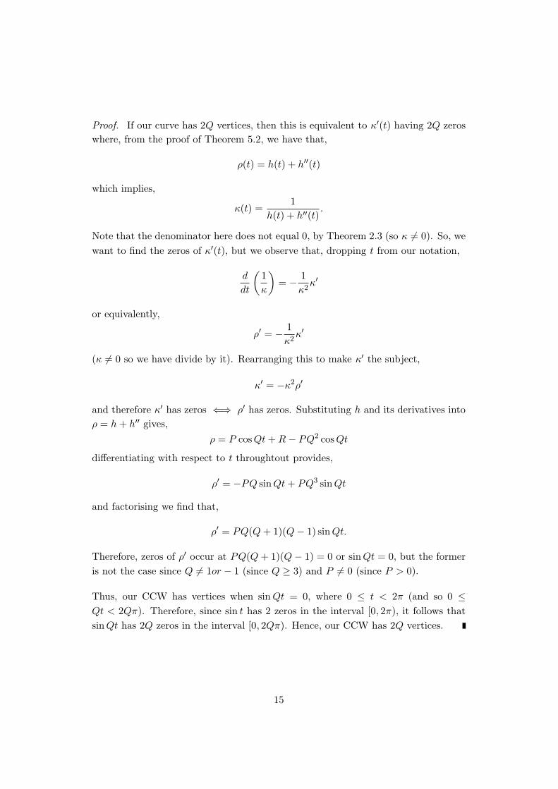
Proof. If our curve has 2Q vertices, then this is equivalent to κ′(t) having 2Q zeroswhere, from the proof of Theorem 5.2, we have that,
ρ(t) = h(t) + h′′(t)
which implies,
κ(t) =1
h(t) + h′′(t).
Note that the denominator here does not equal 0, by Theorem 2.3 (so κ 6= 0). So, we
want to find the zeros of κ′(t), but we observe that, dropping t from our notation,
d
dt
(1κ
)
= −1κ2
κ′
or equivalently,
ρ′ = −1κ2
κ′
(κ 6= 0 so we have divide by it). Rearranging this to make κ′ the subject,
κ′ = −κ2ρ′
and therefore κ′ has zeros ⇐⇒ ρ′ has zeros. Substituting h and its derivatives intoρ = h + h′′ gives,
ρ = P cos Qt + R − PQ2 cos Qt
differentiating with respect to t throughtout provides,
ρ′ = −PQ sin Qt + PQ3 sin Qt
and factorising we find that,
ρ′ = PQ(Q + 1)(Q − 1) sin Qt.
Therefore, zeros of ρ′ occur at PQ(Q + 1)(Q − 1) = 0 or sin Qt = 0, but the former
is not the case since Q 6= 1or − 1 (since Q ≥ 3) and P 6= 0 (since P > 0).
Thus, our CCW has vertices when sin Qt = 0, where 0 ≤ t < 2π (and so 0 ≤
Qt < 2Qπ). Therefore, since sin t has 2 zeros in the interval [0, 2π), it follows that
sin Qt has 2Q zeros in the interval [0, 2Qπ). Hence, our CCW has 2Q vertices.
15
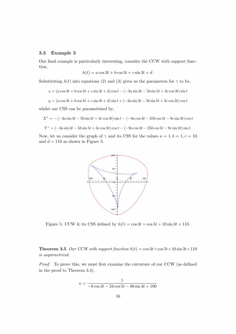
3.3 Example 3
Our final example is particularly interesting, consider the CCW with support func-tion,
h(t) = a cos 3t + b cos 5t + c sin 3t + d.
Substituting h(t) into equations (2) and (3) gives us the parameters for γ to be,
x = (a cos 3t + b cos 5t + c sin 3t + d) cos t − (−3a sin 3t − 5b sin 5t + 3c cos 3t) sin t
y = (a cos 3t + b cos 5t + c sin 3t + d) sin t + (−3a sin 3t − 5b sin 5t + 3c cos 3t) cos t
whilst our CSS can be parametrised by,
X∗ = − (−3a sin 3t − 5b sin 5t + 3c cos 3t) sin t − (−9a cos 3t − 25b cos 5t − 9c sin 3t) cos t
Y ∗ = (−3a sin 3t − 5b sin 5t + 3c cos 3t) cos t − (−9a cos 3t − 25b cos 5t − 9c sin 3t) sin t.
Now, let us consider the graph of γ and its CSS for the values a = 1, b = 1, c = 10and d = 110 as shown in Figure 5.
50
100
0
0
-100
-50 100
-50
50
-100
Figure 5: CCW & its CSS defined by h(t) = cos 3t + cos 5t + 10 sin 3t + 110.
Theorem 3.5 Our CCW with support function h(t) = cos 3t+cos 5t+10 sin 3t+110is asymmetrical.
Proof. To prove this, we must first examine the curvature of our CCW (as defined
in the proof to Theorem 3.4),
κ =1
−8 cos 3t − 24 cos 5t − 80 sin 3t + 100
16
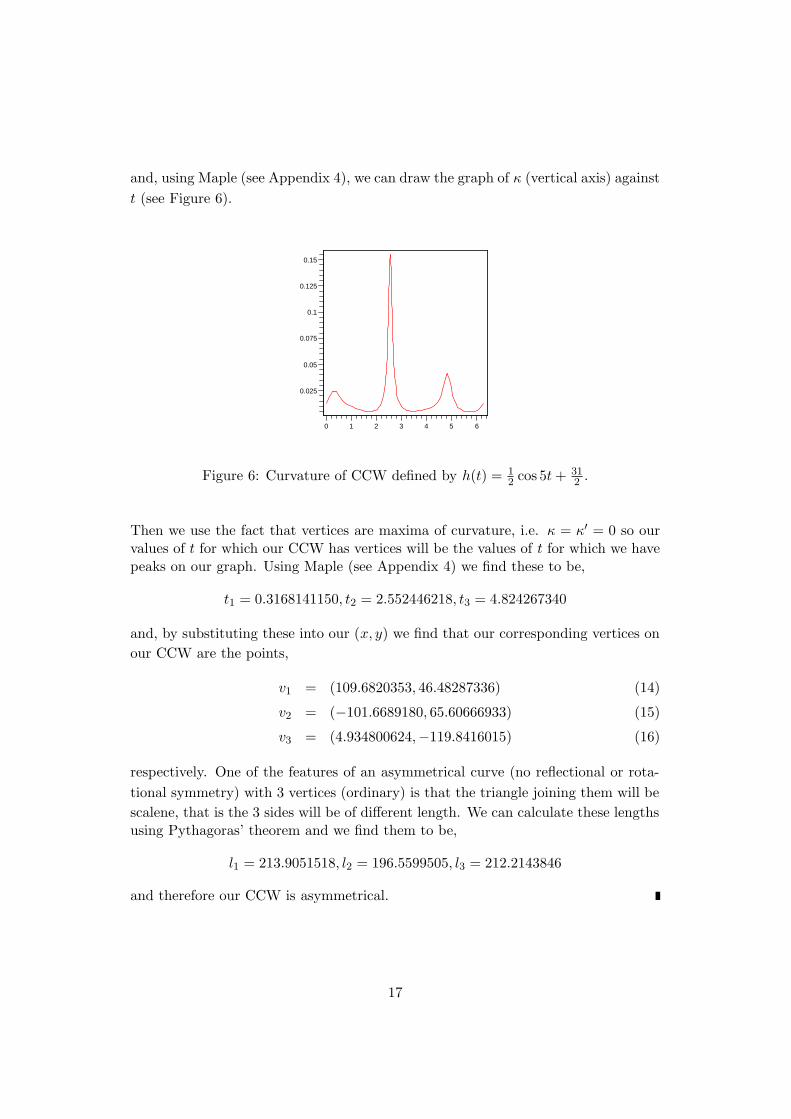
and, using Maple (see Appendix 4), we can draw the graph of κ (vertical axis) against
t (see Figure 6).
6
0.05
2 5
0.075
0.025
1
0.1
0
0.15
0.125
3 4
Figure 6: Curvature of CCW defined by h(t) = 12 cos 5t + 31
2 .
Then we use the fact that vertices are maxima of curvature, i.e. κ = κ′ = 0 so ourvalues of t for which our CCW has vertices will be the values of t for which we havepeaks on our graph. Using Maple (see Appendix 4) we find these to be,
t1 = 0.3168141150, t2 = 2.552446218, t3 = 4.824267340
and, by substituting these into our (x, y) we find that our corresponding vertices onour CCW are the points,
v1 = (109.6820353, 46.48287336) (14)
v2 = (−101.6689180, 65.60666933) (15)
v3 = (4.934800624,−119.8416015) (16)
respectively. One of the features of an asymmetrical curve (no reflectional or rota-
tional symmetry) with 3 vertices (ordinary) is that the triangle joining them will bescalene, that is the 3 sides will be of different length. We can calculate these lengthsusing Pythagoras’ theorem and we find them to be,
l1 = 213.9051518, l2 = 196.5599505, l3 = 212.2143846
and therefore our CCW is asymmetrical.
17

4 Algebraic Expressions
In our section on support functions, we found a parametric expression for our curveγ (we called this (x(t), y(t))) and also for the CSS for γ of constant width (which we
called (X∗, Y ∗)). Now we would like to determine whether the CCW and CSS arealgebraic curves.
4.1 Example 4
Take for example the curve we constructed from the support function in Example 1.Our parameters of γ in that case were,
x =(a
2cos 3t +
a
2+ b)
cos t +3a
2sin 3t sin t
y =(a
2cos 3t +
a
2+ b)
sin t −3a
2sin 3t cos t,
so in order to find an algebraic expression, we need to eliminate our parameter tfrom these equations. This process quickly becomes very complicated, but it can bedone with the help of Maple (see Appendix 5). First of all, simplifying our (x, y)above using Maple’s knowledge of trigonometrical identites gives,
x = −4a cos4 t + 6a cos2 t +a
2cos t + b cos t −
3a
2
y = −12
sin t(8a cos3 t − a − 2b
)
and we notice that here x is expressed completely in terms of cos t but that we havea sin t term in y. In order to eliminate this sin t (we want x, y both expressed in
terms of the same variable), we square y, thus creating a sin2 t term which can be
replaced by 1 − cos2 t and the result is,
y2 =14
(1 − cos2 t
) (64a2 cos6 t − 32ab cos3 t − 16a2 cos3 t + a2 + 4ab + 4b2
).
So we have 2 equations both expressed in terms of the same variable cos t, let thisequal a new variable C, consequently,
x = −4aC4 + 6aC2 +a
2C + bC −
3a
2
y2 =14(1 − C2)
(64a2C6 − 32abC3 − 16a2C3 + a2 + 4ab + 4b2
).
18
If we now eliminate C from these equations (using Maple, see Appendix 5) and usethe same values of a and b as in Example 1, we find that our algebraic equation forour curve γ (of constant width) is,
x8+16x7+19x6+4(x6y2+x2y6)−5544x5−16x5y2−41283(x4+y4)−519x4y2+6y4x4+
266382x3 − 80x3y4 + 11088x3y2 + 7950960x2 + 441x2y4 + 16632y4x − 82566x2y2 −
48y6x − 799146y2x + 7950960y2 − 45y6 + y8 = 373248000
and we notice that this curve is of degree 8.
Using a similar approach, we find that the algebraic expression for the correspondingCSS, previously parametrised by (X∗, Y ∗) where,
X∗ =3a
2sin 3t sin t +
9a
2cos 3t cos t
Y ∗ = −3a
2sin 3t cos t +
9a
2cos 3t sin t
is given by,
X∗4 − 24X∗3 + 162X∗2 + 2X∗2Y ∗2 + 72X∗Y ∗2 + 162Y ∗2 + Y ∗4 = 2187
and we notice that this curve is of degree 4.
In fact, through the observation of other examples, we conjecture that generally,for any support function of the form h(t) = P cos Qt + R, where P and R are someconstants and Q is some odd integer ≥ 3, that its curve γ will have degree 2β + 2and the corresponding CSS has degree β + 1 (half that of the curve).
4.2 Example 5
An interesting question might be: are there other support functions, besides thoseof the form h(t) = P cos 3t + R, which produce a CCW with 6 vertices (and hence a
CSS with 3 cusps)? Well, let us consider the curve with support function,
h(t) = a cos 3t + b cos 5t + c
where b is small and our curve can be parametrised by (x, y) such that,
x = (a cos 3t + b cos 5t + c) cos t − (−3a sin 3t − 5b sin 5t) sin t
y = (a cos 3t + b cos 5t + c) sin t + (−3a sin 3t − 5b sin 5t) cos t
19
and the corresponding CSS can be parametrised by (X∗, Y ∗) such that,
X∗ = − (−3a sin 3t − 5b sin 5t) sin t − (−9a cos 3t − 25b cos 5t) cos 5t
Y ∗ = (−3a sin 3t − 5b sin 5t) cos t − (−9a cos 3t − 25b cos 5t) sin 5t.
Using a similar method to that of Example 4 we find that, by eliminating t fromour equation and by letting a = 1, b = 0.01 and c = 10 we find that our curve isalgebraic with equation,
−1173632.509x − 0.0401768067y6x + 0.0232928689y6x2 + 0.02858369159x4y4
+ 3.117481181x4y2 − 58.37739244x3y2 − 0.03305188292y2x6 + 1.696502092x3y4
− 0.5258350304x5y2 + 116.4626578y4x + 25.86689693y4x2 + 4752.134265y2x
− 1471.699139x2y2 − 1.786474297y6 − 0.6566123013x7 + 0.0004083423248y2x8
+ 0.000013309184y2x9 + 0.0004118065498xy8 + 0.01697225998x8 − 78.37006461x5
+51371.41114x2+1411.175166x4+22533.25936x3−15.10876437x6+0.00664677896y8
− 151.4573255y4 + 0.0000001536y10x2 + 0.000000384y4x8 + 0.000000512y6x6
+ 0.000000384x4y8 + 0.000237166864y6x4 + 0.000101015864y8x2
+ 0.000022987264y4x7 + 0.000019245568y6x5 + 0.00000769664y8x3
+ 0.00000114304y10x + 0.0004329471456y4x6 + 0.004011831741y2x7
+ 0.001954836976y4x5 + 0.0000001536x10y2 + 0.001595414176y6x3
+ 99874.04907y2 + 0.000029166984y10 + 0.003066641175x9 + 0.0001408326026x10
+ 0.000003013888x11 + 0.0000000256y12 + 0.0000000256x12 = 7237792.1
and we can see that this is a curve of degree 12 whilst our CSS has equation,
130.5789041X∗ − 0.0352734375X∗4 + 0.0004X∗6 − 107.3467125X∗
+ 0.02493X∗5 + 128.8374885Y ∗2 + 64.8856125X∗Y ∗2 + 4.445203125X∗2Y ∗2
+ 0.9272765625X∗4 + 0.06705X∗Y ∗4 + 0.0963Y ∗2X∗3 + 0.0012 Y ∗2X∗4
+ 0.0004Y ∗6 + 0.0012Y ∗4X∗2 − 12.74613750X∗3 = 1772.281877
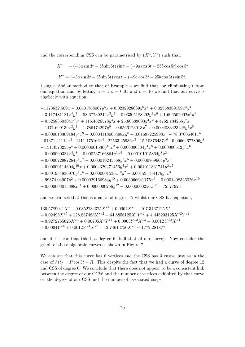
and it is clear that this has degree 6 (half that of our curve). Now consider thegraph of these algebraic curves as shown in Figure 7.
We can see that this curve has 6 vertices and the CSS has 3 cusps, just as in thecase of h(t) = P cos 3t + R. This despite the fact that we had a curve of degree 12and CSS of degree 6. We conclude that there does not appear to be a consistent linkbetween the degree of our CCW and the number of vertices exhibited by that curveor, the degree of our CSS and the number of associated cusps.
20
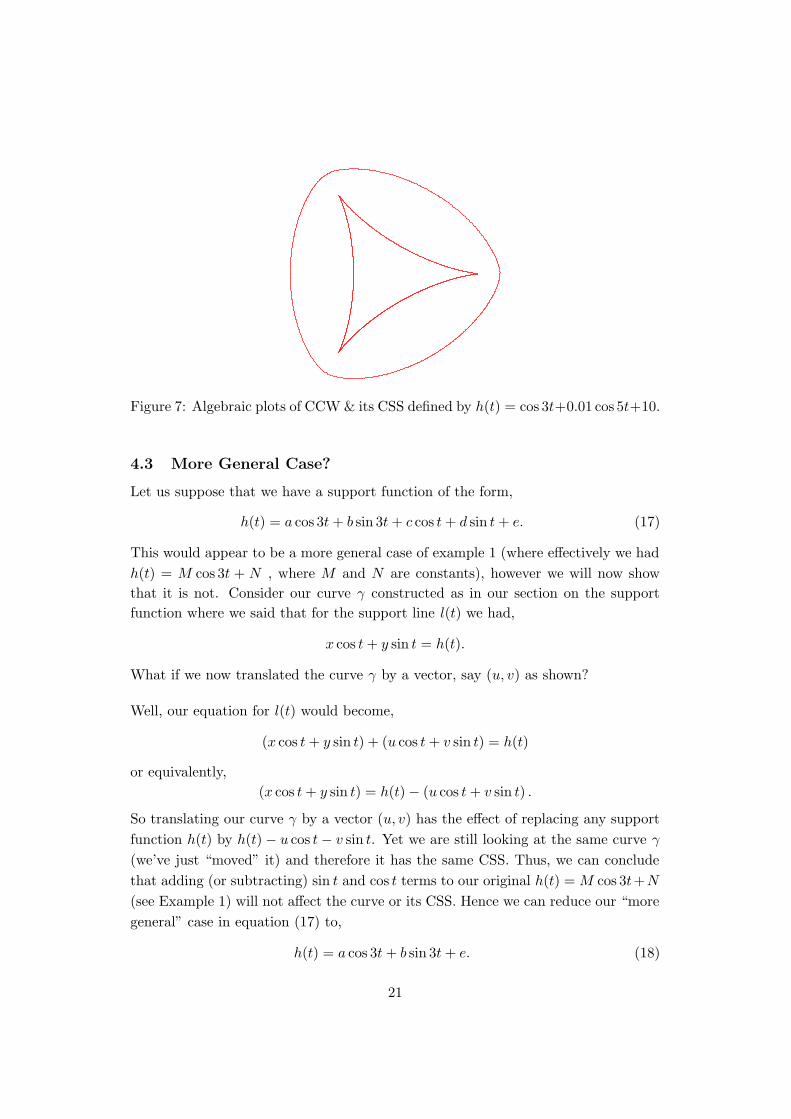
Figure 7: Algebraic plots of CCW & its CSS defined by h(t) = cos 3t+0.01 cos 5t+10.
4.3 More General Case?
Let us suppose that we have a support function of the form,
h(t) = a cos 3t + b sin 3t + c cos t + d sin t + e. (17)
This would appear to be a more general case of example 1 (where effectively we had
h(t) = M cos 3t + N , where M and N are constants), however we will now showthat it is not. Consider our curve γ constructed as in our section on the supportfunction where we said that for the support line l(t) we had,
x cos t + y sin t = h(t).
What if we now translated the curve γ by a vector, say (u, v) as shown?
Well, our equation for l(t) would become,
(x cos t + y sin t) + (u cos t + v sin t) = h(t)
or equivalently,(x cos t + y sin t) = h(t) − (u cos t + v sin t) .
So translating our curve γ by a vector (u, v) has the effect of replacing any support
function h(t) by h(t) − u cos t − v sin t. Yet we are still looking at the same curve γ
(we’ve just “moved” it) and therefore it has the same CSS. Thus, we can conclude
that adding (or subtracting) sin t and cos t terms to our original h(t) = M cos 3t+N
(see Example 1) will not affect the curve or its CSS. Hence we can reduce our “more
general” case in equation (17) to,
h(t) = a cos 3t + b sin 3t + e. (18)
21
t
h(t)
l(t)
(cos t,sin t)
0
γ
v
u
x
y
Now let us see what happens if we rotate the curve γ. We would like to show at thispoint that, given a and b as follows, then there exists A > 0 and α as follows, suchthat the equation below is satisfied,
a cos 3t + b sin 3t = A cos 3(t + α)
(since we are trying to show that (18) can be simplified to h(t) = M cos 3t + N as
claimed at the start of this section). Well, let us expand the RHS of the previousequation,
a cos 3t + b sin 3t = A [cos 3t sin 3α − sin 3t cos 3α]
and, by comparing the coefficients of cos 3t and sin 3t on either side of this equation,we find that,
a = A sin 3α (19)
b = −A cos 3α (20)
By squaring these 2 equations and then adding them together, we can find ourexpression for A,
a2 + b2 = A2
which implies that A =√
a2 + b2. If we now substiute this value for A back into oursimultaneous equations above then we have,
a =√
a2 + b2 sin 3α (21)
b = −√
a2 + b2 cos 3α (22)
22
and these enable us to define our angle α in terms of a and b,
sin 3α =a
√a2 + b2
cos 3α =−b
√a2 + b2
(we always define an angle in terms of its sine and cosine). In conclusion we haveshown that, given a and b there exists A > 0 and α such that a cos 3t + b sin 3t =A cos 3(t + α) so equation (18) can be simplified to,
h(t) = A cos 3t + e. (23)
for rotated axes.
23
5 Barbier’s Theorem
My main reference for this section is [F].
Theorem 5.1 (Barbier) For a closed convex curve of constant width w ≥ 0, itsperimeter is equal to πw.
Proof. Let our curve γ be parametrised by (x, y) = (h(t) cos t−h′(t) sin t, h(t) sin t+
h′(t) cos t) where h(t) represents our support function and ′ represents differentiationwith respect to t. Consider the arc length s defined by,
s =∫ 2π
0
√(dx
dt
)2
+
(dy
dt
)2
.dt
for our case where, from now on we shall write h in place of h(t), h′ instead of h′(t)and so on. We can easily find the following terms,
(dx
dt
)2
=(h2 + 2hh′′ + h′′2
)sin2 t
(dy
dt
)2
=(h2 + 2hh′′ + h′′2
)cos2 t
which when substituted into our equation for s gives,
s =∫ 2π
0
√(h2 + 2hh′′ + h′′2
).dt =
∫ 2π
0
√(h + h′′)2.dt =
∫ 2π
0
(h + h′′) .dt
noting that arc length must be positive. At this point we can use the fact that, ifour curve is of constant width w, then the following poperties hold;
h(t) + h(t + π) = w (24)
h′(t) + h′(t + π) = 0 (25)
h′′(t) + h′′(t + π) = 0. (26)
In order to use these, we split the interval of our integral for s into (0, π) and (π, 2π)as follows,
s =∫ π
0
(h + h′′) .dt +
∫ 2π
π
(h + h′′) .dt
and looking at our second integral, we would like to use a change of variable, lettingu = t − π. Together with the corresponding change of limits this gives us,
s =∫ π
0
(h(t) + h′′(t)
).dt +
∫ π
0
(h(u + π) + h′′(u + π)
).du
24
where ′ here denotes derivatives of the respective variables t and u. Now we want touse our properties above (for variable u rather than t) and rearrange such that thefollowing conditions hold;
h(u + π) = w − h(u) (27)
h′′(u + π) = −h′′(u). (28)
Substituting these into our integral gives us,
s =∫ π
0
(h(t) + h′′(t)
).dt +
∫ π
0
(w − h(u) − h′′(u)
).du
and remember that t and u are just variables so we can combine the 2 integrals,perhaps letting t = u = z for example, so we have that
s =∫ π
0
(h(z) + h′′(z) + w − h(z) − h′′(z)
).dz = πw.
Another interesting theorem relating to a CCW is Theorem 5.2.
Theorem 5.2 The radii of curvature at opposite points(x(t), y(t)) and (x(t + π), y(t + π)) have a constant sum equal to w (w as before).
Proof. As before, let our plane curve γ be a CCW parametrised by,
(x(t), y(t)) = (h(t) cos t − h′(t) sin t, h(t) sin t + h′(t) cos t)
where h(t) represents our support function and ′ represents differentiation with re-spect to t. It follows that,
(x(t + π), y(t + π)) = (−h(t + π) cos t + h′(t + π) sin t,−h(t + π) sin t−h′(t + π) cos t)
and we would like to find the curvature at these points. We can define the curvatureκ at a point on the γ, with arc length s, by the formula,
κ =dt
ds.
Then, since the radius of curvature ρ is the inverse of κ we have that,
ρ =ds
dt=
∣∣∣∣dγ
dt
∣∣∣∣ .
25
So for the radius of curvature at the point (x(t), y(t)), we have
ρ(t) =√
(h′ cos t − h sin t − h′′ sin t − h′ cos t)2 + (h′ sin t + h cos t + h′′ cos t − h′ sin t)2.
where h = h(t). We can see that terms will cancel here leaving,
ρ(t) =√
(−h sin t − h′′ sin t)2 + (h cos t + h′′ cos t)2
which we can then factorise as follows,
ρ(t) =√
[−(h + h′′)(sin t)]2 + [(h + h′′)(cos t)]2
and this simplifies to,
ρ(t) =√
(h + h′′)2(sin2 t + cos2 t) = h + h′′.
Now, in a similar way, let us consider the radius of curvature at the point(x(t + π), y(t + π)), which after cancellation is seen to be,
ρ(t + π) =√
(h(t + π) sin t + h′′(t + π) sin t)2 + (−h(t + π) cos t − h′′(t + π) cos t)2.
Gathering terms together in the same way as we did previously we find that,
ρ(t + π) =√
[(hπ + h′′π) sin t]2 + [−(hπ + h′′
π) cos t]2 = hπ + h′′π.
Therefore, the sum of the radii of curvature at opposite points have sum,
ρ(t) + ρ(t + π) = h(t) + h′′(t) + h(t + π) + h′′(t + π)
and using our properties for a CCW (i.e. h(t)+h(t+π) = w and h′′(t)+h′′(t+π) = 0),this becomes,
ρ(t) + ρ(t + π) = w.
26
6 Morse’s Lemma
My main reference for this section is [BG].
Say we have a closed, non-convex curve Γ, then we can pick out parallel tangentswith the function,
h(t1, t2) = T (t1).N(t2)
where T (ti) is the tangent at Γ(ti) and N(ti) is the normal at Γ(ti) for i = 1 or
2. We use the fact that h(t1, t2) = 0 if the tangent at Γ(t1) is perpendicular to the
normal at Γ(t2) (and therefore the respective tangents are parallel). Clearly, a trivialsolution would arise if t1 = t2 since
h(t1, t2) = T (t1).N(t1) = 0
by definition. We want to find the parameter of points on Γ where the tangents areparallel (either t1 or t2).
First consider the Implicit Function Theorem (taken from MATH443) and the Ja-
cobian of h = h(t1, t2) at the origin (which means t1 = t2) .
Theorem 6.1 (Implicit Function Theorem) Let Rm, v → Rq, c (m ≥ q) be a
smooth map (defined near v ∈ Rm such that f(v) = c) and suppose v is a regular
point of f (J(f) has rank q at v). There are q linearly independent columns of J(f)
at v (non-zero q × q minor).
Then, for mf−1(c) close to v, we can express the variables corresponding to theq independent columns as smooth functions of those remaining.
Let us examine points near (t1, t2) = (0, 0) using the Jacobian matrix,
J(h) =
(∂h
∂t1,∂h
∂t2
)
which gives us that,J(0, 0) = (0, 0)
so J is singular, thus we cannot use the Implicit Function Theorem (IFT) and weresort to the Morse lemma. Instead of using the Jacobian matrix, we use the Hessianmatrix for our function h(t1, t2) = T (t1).N(t2).
DefinitionA Morse function f(t1, t2) mapped by f : R2 → R is one for which ∂f
∂t1= ∂f
∂t2= 0,
27
i.e. f is singular at (t1, t2) and the Hessian matrix,
H(f) =
∂2f∂t21
∂2f∂t1∂t2
∂2f∂t1∂t2
∂2f∂t22
is non-singular at (t1, t2), i.e.
|H(f)| =
∣∣∣∣∣∣
∂2f∂t21
∂2f∂t1∂t2
∂2f∂t1∂t2
∂2f∂t22
∣∣∣∣∣∣6= 0.
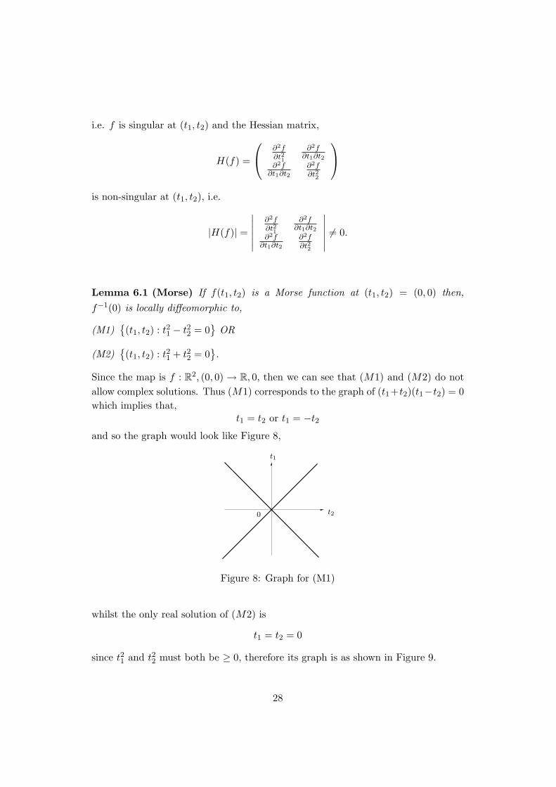
Lemma 6.1 (Morse) If f(t1, t2) is a Morse function at (t1, t2) = (0, 0) then,
f−1(0) is locally diffeomorphic to,
(M1){(t1, t2) : t21 − t22 = 0
}OR
(M2){(t1, t2) : t21 + t22 = 0
}.
Since the map is f : R2, (0, 0) → R, 0, then we can see that (M1) and (M2) do not
allow complex solutions. Thus (M1) corresponds to the graph of (t1+t2)(t1−t2) = 0which implies that,
t1 = t2 or t1 = −t2
and so the graph would look like Figure 8,
t1
t20
Figure 8: Graph for (M1)
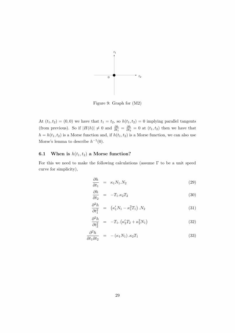
whilst the only real solution of (M2) is
t1 = t2 = 0
since t21 and t22 must both be ≥ 0, therefore its graph is as shown in Figure 9.
28
t1
t20
Figure 9: Graph for (M2)
At (t1, t2) = (0, 0) we have that t1 = t2, so h(t1, t2) = 0 implying parallel tangents
(from previous). So if |H(h)| 6= 0 and ∂h∂t1
= ∂h∂t2
= 0 at (t1, t2) then we have that
h = h(t1, t2) is a Morse function and, if h(t1, t2) is a Morse function, we can also use
Morse’s lemma to describe h−1(0).
6.1 When is h(t1, t2) a Morse function?
For this we need to make the following calculations (assume Γ to be a unit speed
curve for simplicity),
∂h
∂t1= κ1N1.N2 (29)
∂h
∂t2= −T1.κ2T2 (30)
∂2h
∂t21=
(κ′
1N1 − κ21T1
).N2 (31)
∂2h
∂t22= −T1.
(κ′
2T2 + κ22N1
)(32)
∂2h
∂t1∂t2= − (κ1N1) .κ2T1 (33)
29

where κ′i means the derivative of κ(ti) with respect to ti for i = 1 or 2. Let us
consider the example of (t1, t2) = (0, 0) so that we might use Morse’s Lemma.
∂h
∂t1= κ(0)N(0).N(0) = κ(0) (34)
∂h
∂t2= −T (0).κ(0)T (0) = −κ(0) (35)
∂2h
∂t21=
(κ′(0)N(0) − κ(0)2T (0)
).N(0) = κ′(0) (36)
∂2h
∂t22= −T (0).
(κ′(0)T (0) + κ(0)2N(0)
)= −κ′(0) (37)
∂2h
∂t1∂t2= − (κ(0)N(0)) .κ(0)T (0) = 0 (38)
and so since for a Morse function, we require ∂h∂t1
= ∂h∂t2
= 0, we can see that
κ(0) = −κ(0) = 0, i.e. we have an inflexion at the origin. Our correspondingHessian matrix would be,
H(0, 0) =
(κ′(0) 0
0 −κ′(0)
)
and we know that a Morse function requires this to be non-singular, i.e. we must
have that −κ′ (0)2 6= 0. In fact, if this is the case, then κ′(0) 6= 0 and so we
have that −κ′ (0)2 < 0. This means that our condition for a Morse function when
(t1, t2) = (0, 0) is that,
κ(0) = 0 & κ′(0) 6= 0
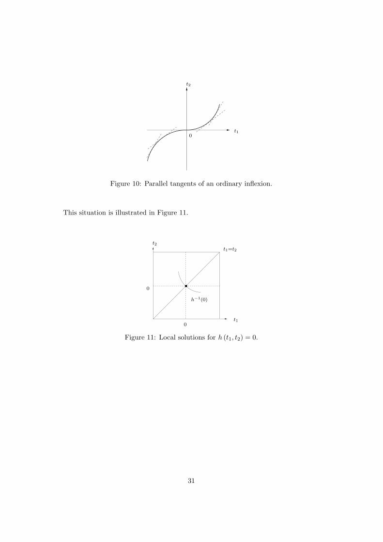
i.e. an ordinary inflexion at the origin. The parallel tangents of a curve with anordinary inflexion at (t1, t2) = (0, 0) would not only occur for our trivial solution
(t1 = t2), but also for t1 6= t2 when near the origin (see Figure 10).
The set h−1(0) can be reprsented by Figure 11, i.e. h−1(0) has a local solutioncomprising a pair of 2 intersecting curves, one of which is the diagonal t1 = t2
(which is clearly smooth). We have found that h−1(0) is locally a pair of smoothtransverse curves, using the Morse lemma; hence the true parallel tangent set is the
other smooth branch of h−1(0) besides the diagonal.
Proposition 6.1 In a neighbourhood of an ordinary inflexion, the parallel tangentset is a smooth curve.
30
t1
t2
0
Figure 10: Parallel tangents of an ordinary inflexion.
This situation is illustrated in Figure 11.
t1
t2t1=t2
0
0
h−1(0)
Figure 11: Local solutions for h (t1, t2) = 0.
31

7 Reconstruction of a curve from its CSS
We would like to find out if, given a curve, say A parametrised by A(s) = (h(s), s)
and another piece of curve, say B parametrised by B(u) = (u, q + g(u)), is it possible
to find another piece of curve, say C parametrised by C(t) = (t, p + f(t)) such thatB and C have A as their CSS?
A
B
C
p
q
A(s)
B(u)
C(t)
Figure 12: Curve A is the CSS to curves B and C here.
Here the dotted lines at the top and bottom of the diagram represent parallel tan-gents at B(u) and C(t) whilst the dashed line joining them is tangential to A. Also,
the constants p and q are equal to the distances between the tangent points C(t) and
B(u) respectively (represented by black circles on C and B) and the tangent point
on A (represented by black circle on A). We have some conditions for our problem.
Firstly, we want B(u) and C(t) to lie on the tangent to A(s) and secondly, we
want g′(u) = f ′(s), i.e. we want the tangents to B and C to be parallel (′ here
denotes differentiation with respect to the specified variable, as it will throughout).
We would expect t and u to be functions of s since the points B(u) and C(t) lie onthe tangent to the curve A, parametrised by the variable s.
Using our first condition we have,
(u, q + g(u)) = (h(s), s) + μ(h′(s), 1
)(39)
(t, p + f(t)) = (h(s), s) + λ(h′(s), 1
)(40)
and we want all of the fuctions here (g, f and h) to be functions of s (variable of the
CSS to curve B) so that, knowing only B and its CSS A, we can find C.
32
Well, we know that h is a function of s and, implicitly, we have that u is a function ofs (B(u) lies on the tangent to A(s) since A is the CSS to B) and therefore g = g(u)is a function of s. Now we want to find t, the variable of curve C, as a function ofs, and thus f = f (t (s)). So, rearranging equations (39) and (40) we find,
(u, q + g(u)) − (h(s), s) = μ(h′(s), 1
)
(t, p + f(t)) − (h(s), s) = λ(h′(s), 1
)
and now, if we think of these in terms of (x, y) coordinates and we divide the x
coordinates by the y coordinates then we obtain the following,
u − h(s)q + g(u) − s
= h′(s) (41)
t − h(s)p + f(t) − s
= h′(s) (42)
noticing that we have eliminated μ and λ. If we now consider equation (41) to be a
family of chords (joining B(u) to A(s)), say G(s, u) where,
G(s, u) = u − h(s) − h′(s) (q + g(u) − s) .
Since our model is affinely invariant, we can take an affine transformation, i.e. we canset up our model in such a way that we can take a point on A to be the origin (such
that A(s) = (h(s), s) = (0,0)) and let the tangent to A at that point, parametrised
by (h′(s), 1), be the vertical axis (represented by the dashed line in Figure 12).
We can then let this vertical tangent intersect with curve B at the point where itsparameter u also equals 0 and such that the tangent to B at this point, parametrisedby (1, g′(u)), is a horizontal tangent i.e. we analyse our given curves A and B at thepoints with parameter value 0.
So now, let us consider the Jacobian matrix,
J =
(∂G
∂s,∂G
∂u
)
close to (s, u) = (0, 0). We have that,
∂G
∂u= 1 − h′(s)g′(u)
and we have set up our model in such a way that h(0) = h′(0) = 0 (and g′(0) = 0)so then,
∂G
∂u(0, 0) = 1 6= 0
33
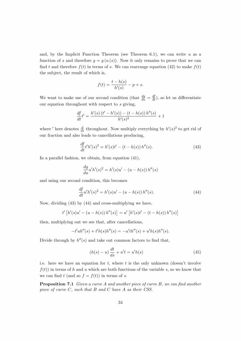
and, by the Implicit Function Theorem (see Theorem 6.1), we can write u as a
function of s and therefore g = g (u (s)). Now it only remains to prove that we can
find t and therefore f(t) in terms of s. We can rearrange equation (42) to make f(t)the subject, the result of which is,
f(t) =t − h(s)h′(s)
− p + s.
We want to make use of our second condition (that dgdu = df
dt ), so let us differentiate
our equation throughout with respect to s giving,
df
dtt′ =
h′(s) (t′ − h′(s)) − (t − h(s)) h′′(s)h′(s)2
+ 1
where ′ here denotes dds throughout. Now multiply everything by h′(s)2 to get rid of
our fraction and also leads to cancellations producing,
df
dtt′h′(s)2 = h′(s)t′ − (t − h(s)) h′′(s). (43)
In a parallel fashion, we obtain, from equation (41),
dg
duu′h′(s)2 = h′(s)u′ − (u − h(s)) h′′(s)
and using our second condition, this becomes
df
dtu′h′(s)2 = h′(s)u′ − (u − h(s)) h′′(s). (44)
Now, dividing (43) by (44) and cross-multiplying we have,
t′[h′(s)u′ − (u − h(s)) h′′(s)
]= u′ [h′(s)t′ − (t − h(s)) h′′(s)
]
then, multiplying out we see that, after cancellations,
−t′uh′′(s) + t′h(s)h′′(s) = −u′th′′(s) + u′h(s)h′′(s).
Divide through by h′′(s) and take out common factors to find that,
(h(s) − u)dt
ds+ u′t = u′h(s) (45)
i.e. here we have an equation for t, where t is the only unknown (doesn’t involve
f(t)) in terms of h and u which are both functions of the variable s, so we know that
we can find t (and so f = f(t)) in terms of s.
Proposition 7.1 Given a curve A and another piece of curve B, we can find anotherpiece of curve C, such that B and C have A as their CSS.
34
7.1 Example 6
Let our function h(s) = s2, so that our CSS curve A is parametrised by,
A(s) =(s2, s
)
and similarly, let our function g(u) = αu2 so that our given piece of curve B isparametrised by,
B(u) =(u, q + αu2
).
We don’t know an explicit value for t but we do know that it can be expressed interms of s, so express t as a power series in s up to degree 5,
t = t1s + t2s2 + t3s
3 + t4s4 + t5s
5
and similarly, let us describe f as a power series in t as follows,
f = f2t2 + f3t
3 + f4t4 + f5t
5
where ti and fi for 1 ≤ i ≤ 5 are coefficients to be found. However, we have an
equation for t in (45), but for this we need explicit expressions for u and duds . So, by
rearranging equation (41), we have,
u − h(s) − h′(s) (q + g(u) − s) = 0
and, by substituting our values from A(s) above into this, we find that s2 termscancel to give,
u − 2sq − 2sαu2 + s2 = 0
i.e. we have a quadratic equation in u, so using the quadratic formula we have that,
u =1 ±
√1 − 8s2α (2q − s)
4sα
and we want to choose the sign (+ or −) which gives a finite value for u(0) when weexpress our square root term as a power series in s. It is clear that we must take u−,
since if we took u+ our first term in the power series for u(s) would be 12sα which
would be infinite when s = 0. Now, using Maple (see Appendix 6) we find u and duds
up to degree 5,
u = 2qs − s2 + 8αq2s3 − 8αqs4 +2α2 + 64α3q3
αs5
anddu
ds= 2q − 2s + 24αq2s2 − 32αqs3 +
10α2 + 320α3q3
αs4
35

which we can then substitute into g(u) in order to apply the parallel tangents con-
dition, that is dfdt −
dgdu = 0. Using Maple (see Appendix 6), we can write this as a
power series,
(2f2t1 − 4αq) s +(2f2t2 + 2α + 3f3t
21
)s2 +
(−16α2q2 + 2f2t3 + 6f3t1t2 + 4f4t13
)s3
+(2f2t4 + 16α2q + 3f3
(2t1t3 + t22
)+ 12f4t
21t2 + 5f5t
41
)s4
+(2f2t5 + 3f3 (2t1t4 + 2t2t3) − 4α2 − 128α3q3 + 4f4
(t1(2t1t3 + t22
)+ t3t
21 + 2t22t1
)
+ 20f5t31t2)s5
then we wish to utilise equation (42), expressing it as a series in s. First we re-arrange it to the form
(t − h(s)) − h′(s) (p + f(t) − s) = 0
into which we can then substitute our chosen value of h(s) and our power series
expansions of t and f(t) giving us, in ascending powers of s, the following series.
(t1 − 2p) s + (t2 + 1) s2 +(−2f2t
21 + t3
)s3 +
(t4 − 4f2t1t2 − 2f3t
31
)s4 +
(t5 − 2f2
(2t1t3 + t22
)− 2f4t
41 − 6f3t
21t2)s5
We say that these 2 series are satisfied for any s, so we equate the coefficientsof powers of s to 0 in order to find our ti and fi coefficients, for 1 ≤ i ≤ 5. Thesecalculations (see Appendix 6) heed results from which we can say that,
t(s) = 2ps − s2 + 8αqps3 −
(163
αq +83αp
)
s4 + 2α(32pαq2 + 1
)s5
f (t(s)) = 4αqps2 −43α (2q + p) s3 + α
(32pαq2 + 1
)s4 −
1615
α2q (23p + 22q) s5.
So now, by assigning numerical values to α, p and q, we can use Maple (see Appendix
7) to draw curves A, B and C and their tangents (see Figure 13).
Here we have let α = 1, p = 2 and q = −2 and the “middle”curves represent A,the “lower”curves represent B whilst the “upper”curves represent C (very much as
depicted in Figure 12). The thinner lines here represent tangents to our curves, we
can see that the tangents to A join the parallel tangents of B and C (and so A is
the CSS of B and C). This is emphasised in Figure 14 where we have drawn the
tangents for 3 different values of s (s = 0, s = 0.05 and s = −0.05) together.
In future work, we intend to look at surfaces of constant width, together with CSSs in3 dimensions. Also, we would like to see just how far we can take our reconstruction
36
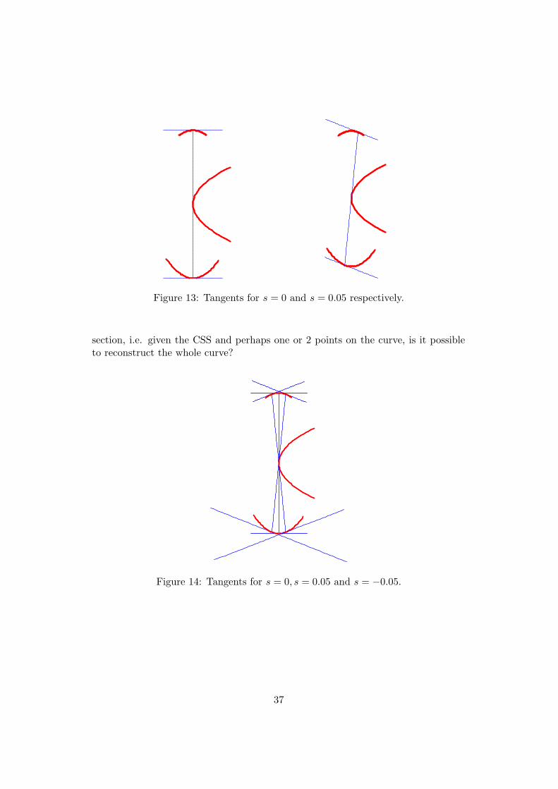
Figure 13: Tangents for s = 0 and s = 0.05 respectively.
section, i.e. given the CSS and perhaps one or 2 points on the curve, is it possibleto reconstruct the whole curve?
Figure 14: Tangents for s = 0, s = 0.05 and s = −0.05.
37

8 Maple Appendices
8.1 Appendix 1
This is the Maple programme for finding the parametrisation of the CSS of a curve,not necessarily of constant width.with(plots):with(plottools):
with(linalg):with(PDEtools):
Consider the support function defined by h(t) and h(t + π) to be defined by h1(t).declare(h(t),h1(t),prime=t):
dh:=diff(h(t),t);dh1:=diff(h1(t),t);d2h:=diff(dh(t),t);Note, whenever using h or h1, we must refer to them as h(t) and h1(t) respec-tively, otherwise Maple will not differentiate them properly. Consider our curveparametrised by (x(t), y(t)) as follows.x:=h(t)*cos(t)-dh*sin(t);y:=h(t)*sin(t)+dh*cos(t);
Now consider (x(t + π), y(t + π)) to be defined by (x1(t), y1(t)).x1:=-h1(t)*cos(t)+dh1*sin(t);y1:=-h1(t)*sin(t)-dh1*cos(t);
Our family of chords can be defined by F .F:=(Y-y)*(x1-x)-(X-x)*(y1-y);
For the envelope of chords we need dFdt .
dF:=diff(F,t);
The envelope of chords is given by the solution to the equations F = dFdt = 0.
XY:=solve({F=0,dF=0},{X,Y});We can say that X is the 2nd of the 2 arguments produced (it could be the 1st).X:=op(2,XY[2]);
and Y is the 1st of the 2 arguments produced (it could be the 2nd).Y:=op(2,XY[1]);
Here (X, Y ) are parameters of the CSS.
8.2 Appendix 2
This picks up where Appendix 1 left off and finds the parametrisation of the CSSwhen we have a CCW. If our curve is of constant width, then we should have certainconditions satisfied;(1) that h(t) + h(t + π) = k where k = constant,X1:=subs(h1=k-h,X);Y1:=subs(h1=k-h,Y);(2) that h′(t) + h′(t + π) = 0,X2:=subs(diff(h1(t),t)=-dh,X1);Y2:=subs(diff(h1(t),t)=-dh,Y1);(3) that h′′(t) + h′′(t + π) = 0 andX3:=subs(diff(diff(h1(t),t),t)=-d2h,X2);Y3:=subs(diff(diff(h1(t),t),t)=-d2h,Y2);(4) that since k = constant, then k′(t) = 0.
38
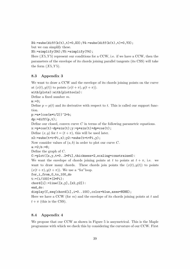
X4:=subs(diff(k(t),t)=0,X3);Y4:=subs(diff(k(t),t)=0,Y3);but we can simplify these.X5:=simplify(X4);Y5:=simplify(Y4);
Here (X5, Y 5) represent our conditions for a CCW, i.e. if we have a CCW, then the
parameters of the envelope of its chords joining parallel tangents (its CSS) will take
the form (X5, Y 5).
8.3 Appendix 3
We want to draw a CCW and the envelope of its chords joining points on the curveat (x(t), y(t)) to points (x(t + π), y(t + π)).with(plots):with(plottools):
Define a fixed number m.m:=3;Define p = p(t) and its derivative with respect to t. This is called our support func-tion.p:=a*(cos(m*t/2))^2+b;
dp:=diff(p,t);
Define our closed, convex curve C in terms of the following parametric equations.x:=p*cos(t)-dp*sin(t);y:=p*sin(t)+dp*cos(t);
Define (x, y) for t = (t + π), this will be used later.x2:=subs(t=t+Pi,x);y2:=subs(t=t+Pi,y);
Now consider values of (a, b) in order to plot our curve C.a:=2;b:=8;Define the graph of C.C:=plot([x,y,t=0..2*Pi],thickness=2,scaling=constrained):
We want the envelope of chords joining points at t to points at t + π, i.e. wewant to draw many chords. These chords join points the (x(t), y(t)) to points
(x(t + π), y(t + π)). We use a “for”loop.for_i_from_0_to_100_dot:=(i/100)*(2*Pi):chord[i]:=line([x,y],[x2,y2]):end_do:display(C,seq(chord[i],i=0..100),color=blue,axes=NONE);
Here we have a CCW (for m) and the envelope of its chords joining points at t and
t + π (this is the CSS).
8.4 Appendix 4
We propose that our CCW as shown in Figure 5 is assymetrical. This is the Mapleprogramme with which we check this by considering the curvature of our CCW. First
39
define the curvature.kappa:=1/(h+d2h);
Then substitute the values for our specific support function.kappa1:=subs(a=a1,b=b1,c=c1,d=d1,kappa);
Define the derviative of κ with respect to t.dkappa:=diff(kappa1,t);
Plot the graph of curvature κ against tplot([t,kappa1,t=0..2*Pi]);
Let t1, t2 and t3 be our maxima of curvature.t1:=fsolve(dkappa=0,t=0..1);
t2:=fsolve(dkappa=0,t=2..3);
t3:=fsolve(dkappa=0,t=4..5);
Now consider the corresponding points on our curve (for these values of t).xx1:=evalf(subs(t=t1,x1));yy1:=evalf(subs(t=t1,y1));
xx2:=evalf(subs(t=t2,x1));yy2:=evalf(subs(t=t2,y1));
xx3:=evalf(subs(t=t3,x1));yy3:=evalf(subs(t=t3,y1));
Now consider the lengths of the sides of a triangle formed by joining these points.len1:=sqrt((xx2-xx3)^2+(yy2-yy3)^2);
len2:=sqrt((xx3-xx1)^2+(yy3-yy1)^2);
len3:=sqrt((xx1-xx2)^2+(yy1-yy2)^2);
8.5 Appendix 5
We would like to derive algebraic equations for a CCW and its CSS.with(linalg):with(plots):with(plottools):
Define our support function and its derivatives. We would like to consider h =
a(cos 3t
2
)2+ b but using the formula cos 2A = 2cos2A − 1 we can simplify this as
follows.h:=a/2*cos(3*t)+a/2+b;dh:=diff(h,t);d2h:=diff(dh,t);Use these to obtain the parameters of our curve.x:=h*cos(t)-dh*sin(t);y:=h*sin(t)+dh*cos(t);
Use Maple’s knowledge of trigonometric identities to simplify our expressions.x1:=simplify(x);simplify(y);
Notice that our equation for x is purely in terms of cos t whilst we have an unwanted
sin t in our expression for y. If we square our equation for y then we will have a sin2 t
term which we can then replace by 1 − cos2 t.y1:=simplify(y^2);
Now we can see that for x1 and y1 (which = y2) we have 2 polynomials all in terms
of cos t (once we’ve used sin2 t = 1 − cos2t in y1).x2:=subs(cos(t)=C,x1);
40
y2:=subs(cos(t)=C,(sin(t))^2=1-C^2,y1);
So now we have 2 equations in terms of the 3 unknowns (x2, y2 and C) so we want
to eliminate C (the variable we don’t want). Use Y Y here since we are looking at
y2, not y.elim1:=eliminate({X=x2,YY=y2},C);
The 1st component above gives us a value of C and the 2nd component is the remain-ing equation, now that C has been eliminated. So we want this 2nd component, usethe following command (note that the 1 in the brackets here gets rid of the brackets
in the output of the command above for us).elim2:=op(1,op(2,elim1))/a;
Now we would like to replace Y Y by Y 2.elim3:=subs(YY=Y^2,elim2);This is our algebraic equation for a CCW! We would like to study the graph of this,so let us consider our equation for the following values of a and b.a1:=2;b1:=8;Substitute these values into our elimination.eq1:=subs(a=a1,b=b1,elim3);
Simplify it.eq2:=(eq1)/(-16);
Notice that this equation is of degree 8 (perhaps since we had 3t in our h(t) and this
is 2 × 3 + 2). Plot the algebraic graph.implicitplot(eq1=0,X=-10..10,Y=-10..10,grid=[100,100]);
But, is this the same as the graph defined by our parametric equations? Definenon-algebraic parameters,x1:=subs(a=a1,b=b1,x);y1:=subs(a=a1,b=b1,y);
and plot them.plot1:=plot([x1,y1,t=0..2*Pi],scaling=constrained):
display(plot1);
The graphs are indeed the same and it would seem that squaring y has not intro-duced any extra components! Now we would like to obtain an algebraic expressionfor the corresponding CSS (we do this in a parallel fashion to the way we did it for
our CCW). Remember we know the parametrisation of the CSS for a CCW.cx:=-dh*sin(t)-d2h*cos(t);cy:=dh*cos(t)-d2h*sin(t);
We can simplify these.cx1:=simplify(cx);cy1:=simplify(cy^2);
cx2:=subs(cos(t)=C,cx1);cy2:=subs(cos(t)=C,(sin(t))^6=(1-C^2)^3,cy1);
Notice that we have 2 equations whose RHSs are expressed completely in terms of
C2. So consider them in terms of a new variable, say CC = C2.cxx2:=subs(C^2=CC,C^4=CC^2,cx2);cyy2:=subs(C^2=CC,cy2);
elim4:=eliminate({CX=cxx2,CYY=cyy2},CC);
elim5:=op(1,op(2,elim4))/a;
41
elim6:=subs(CYY=CY^2,elim5);This is our algebraic expression for the CSS. Notice that this equation is of degree4 (notably half that of the curve itself). Also since the parametrisation of the CSS
did not depend on b (since parametrisation depends on dh and d2h, not h), it is
right that our equation does not either. Consider this for values of a and b (where
a = 2, b = 8 as before).eq2:=subs(a=a1,b=b1,elim6);
eq3:=(eq2)/(-16);
implicitplot(eq2=0,CX=-9..9,CY=-8..8,grid=[200,200]);
cx2:=subs(a=a1,b=b1,cx);cy2:=subs(a=a1,b=b1,cy);
plot2:=plot([cx2,cy2,t=0..Pi],scaling=constrained):
display(plot2);
The graphs are indeed the same and it would seem that squaring cy has not intro-duced any extra components!
8.6 Appendix 6
This is the Maple programme for the reconstruction section. Firstly, we define t asa power series in s.t:=t1*s+t2*s^2+t3*s^3+t4*s^4+t5*s^5;Then we define h(s) and its derivative, for example let,h:=s^2;dh:=diff(h,s);Defining g(u) (and its derivative) allows us to change it later. For example let,g:=alpha*u^2;dg:=diff(g,u);
Define f(t) as a power series in t,f:=f2*t^2+f3*t^3+f4*t^4+f5*t^5;We know that u(s) is the solution of the following equation,u_sol:=solve(u-h-dh*(q+(subs(s=u,g))-s)=0,u);
We need to choose the solution which is 0 at s = 0, this is u− (as apposed to u+).u_val:=u_sol[2];We can now express u(s) as a power series in s.u_val_5:=series(u_val,s,7);Find the derivative of u(s), i.e. u′(s),du:=diff(u_val_5,s);We know that t′(0) = t1 (this is one of our B.C.s along with t(0) = 0). We have 3
main conditions (of which we only need 2 for now).
Condition (1) says f ′(t) = g′(u) i.e. our 2 pieces of curve have parallel tangents.eq1:=series(2*f2*t+3*f3*t^2+4*f4*t^3+5*f5*t^4-subs(u=u_val_5,dg),s,6);
Condition (2) says (t − h) − h′(p + f − s) = 0 i.e. points on our piece of curve wewish to derive, are points on tangent line to CSS curve.
42

eq2:=series((t-h)-dh*(p+f-s),s,6);
We can see that by equating coefficients of powers of s to 0 in eq3, we can find t1and t2.t1_val:=solve(coeff(eq2,s)=0,t1);t2_val:=solve(coeff(eq2,s^2)=0,t2);
Substitute these known values into eq1 and eq2.eq1a:=subs(t1=t1_val,t2=t2_val,eq1);
eq2a:=subs(t1=t1_val,t2=t2_val,eq2);
Now do the same to solve for other t coefficients and f coefficients too.f2_val:=solve(coeff(eq1a,s)=0,f2);
Repeat the process.eq1b:=subs(f2=f2_val,eq1a);eq2b:=subs(f2=f2_val,eq2a);
We can see that we can find f3 from eq1b and t3 from eq2b (since they won’t be interms of other, as yet, unknown coefficients.f3_val:=solve(coeff(eq1b,s^2)=0,f3);
t3_val:=solve(coeff(eq2b,s^3)=0,t3);
eq1c:=subs(f3=f3_val,t3=t3_val,eq1b);
eq2c:=subs(f3=f3_val,t3=t3_val,eq2b);
Notice that the coefficient of s2 in eq1c does equal 0 (for some reason Maple doesn’t
realise)! If this had not been the case then we would have had that p, q were notarbitrary.f4_val:=solve(coeff(eq1c,s^3)=0,f4);
t4_val:=solve(coeff(eq2c,s^4)=0,t4);
eq1d:=subs(f4=f4_val,t4=t4_val,eq1c);
eq2d:=subs(f4=f4_val,t4=t4_val,eq2c);
Again, notice that the coefficient of s4 in eq2d does equal 0!f5_val:=solve(coeff(eq1d,s^4)=0,f5);
t5_val:=solve(coeff(eq2d,s^5)=0,t5);
So now we have all of our f and t coefficients explicitly, sub these into their respec-tive equations. Do t first, since f = f(t).t_val:=subs(t1=t1_val,t2=t2_val,t3=t3_val,t4=t4_val,t5=t5_val,t);f_val:=subs(f2=f2_val,f3=f3_val,f4=f4_val,f5=f5_val,t=t_val,f);Try simplifying this.f_val2:=simplify(f_val);
The way to get a nicer expression for f is to find the series, simplify and find theseries again.f_val2a:=series(simplify(series(f_val2,s,6)),s,6);
8.7 Appendix 7
This is the Maple programme for constructing our 3 pieces of curve A, B and C suchthat B and C have A as their CSS. We need to use certain packages when plotting
43
graphs which we have to call.with(plots):with(plottools):
Consider a piece of curve A, parametrised by (h(s), s), this will represent our CSS.h:=s^2;Define the graph of Aplot1:=plot([h,s,s=-1..1],thickness=3,scaling=constrained):
and then to display the graph, we use the following command.display(plot1);
Now we wish to consider a piece of curve B, parametrised by (u, q + g(u)).g:=alpha*u^2;
From previous calculations, we have an expression for u.u:=2*q*s-s^2+8*alpha*q^2*s^3-8*alpha*q*s^4-1/4*
(-8*alpha^2-256*alpha^3*q^3)*s^5/alpha;
For B we want q + g(u) as the “y”coordinate.By:=q+g;
Give some values to our parameters.q1:=-2;alpha1:=1;
Substitute these into our expressions for u, g and By.u1:=subs(q=q1,alpha=alpha1,u);
g1:=subs(q=q1,alpha=alpha1,g);
u2:=subs(q=q1,alpha=alpha1,g=g1,By);
Then define the graph of B.plot2:=plot([u1,u2,s=-0.2..0.2],thickness=3,scaling=constrained):
Now we seek a 3rd piece of curve, say C, parametrised by (t, p + f(t)). Give anumerical value to parameter p.p1:=2;
We found t(s) to be as follows.t:=2*p*s-s^2+8*alpha*q*p*s^3-(16/3)*alpha*q*s^4-
(8/3)*alpha*p*s^4+2*alpha*32*p*alpha*q^2*s^5+2*alpha*s^5;
And we found f (t(s)).f:=4*alpha*q*p*s^2-4/3*alpha*(2*q+p)*s^3+alpha
*(32*p*alpha*q^2+1)*s^4-16/15*alpha^2*q*(22*q+23*p)*s^5;
For curve C we want p + f(t) as the “y”coordinate.Cy:=p+f;
Substitute our parameter values into these functions.t1:=subs(p=p1,alpha=alpha1,q=q1,t);
f1:=subs(p=p1,alpha=alpha1,q=q1,f);
t2:=subs(p=p1,alpha=alpha1,q=q1,f=f1,Cy);
Define the graph of C.plot3:=plot([t1,t2,s=-0.1..0.1],axes=NONE,
thickness=3,scaling=constrained):
44
Now we want to draw a line which is tangent to A. Let us begin by drawing a singletangent to a point on A, say where s = 0, call this point s0.s0:=0;We can see that the tangent must pass through (As0h
, As0s). This is our point ofcontact on A.A_s0_h:=subs(s=s0,h);A_s0_s:=subs(s=s0,s);We need the derivative of the path (w.r.t. s) of (h(s), s), call these dh and ds
respectively.dh:=diff(h,s);ds:=diff(s,s);So when s = s0, the tangent vector must be (Ts0h
, Ts0s).T_s0_h:=subs(s=s0,dh);T_s0_s:=subs(s=s0,ds);A parametrisation of the tangent line is (TLs0h
, TLs0s).TL_s0_h:=A_s0_h+(s-s0)*T_s0_h;TL_s0_s:=A_s0_s+(s-s0)*T_s0_s;Define the plot of the tangent to A.tan0:=plot([TL_s0_h,TL_s0_s,s=-2..2],axes=NONE,
color=blue,thickness=1,scaling=constrained):
We want to draw the tangent to the point of contact on B. We can see that thistangent must pass through (Bs0u1 , Bs0u2).B_s0_u1:=subs(s=s0,u1);B_s0_u2:=subs(s=s0,u2);We need the derivative of the path (w.r.t. s) of (u1, u2), call these du1 and du2
respectively.du1:=diff(u1,s);du2:=diff(u2,s);So when s = s0, the tangent vector must be (Ts0u1 , Ts0u2).T_s0_u1:=subs(s=s0,du1);T_s0_u2:=subs(s=s0,du2);A parametrisation of the tangent line to B is (TLs0u1 , TLs0u2).TL_s0_u1:=B_s0_u1+(s-s0)*T_s0_u1;TL_s0_u2:=B_s0_u2+(s-s0)*T_s0_u2;Define the tangent to B.tan1:=plot([TL_s0_u1,TL_s0_u2,s=-0.2..0.2],color=blue,
thickness=1,scaling=constrained):
We find the parallel tangent to this on C by multiplying by -1 (by the way we have
set up our model).tan2:=plot([-1*TL_s0_u1,-1*TL_s0_u2,s=-0.2..0.2],
color=blue,thickness=1,scaling=constrained):
To view the 3 curves and their respective tangents, we use the following command.display(plot1,plot2,plot3,tan0,tan1,tan2);
Now consider another value of s, say s1 = 0.05 and find the tangents to A, B and Cin a parallel fashion to the way we did for s0.
45
9 Bibliography
References
[CGI] Ke Chen, Peter Giblin and Alan Irving. Mathematical Explorations with
MATLAB. Cambridge University Press (May 1999), 122 – 127.
[F] J.Chris Fisher. Curves of Constant Width from a Linear Viewpoint. Math-
ematics Magazine Vol. 6 No. 3 (June 1987), 131 - 140.
[BG] J.W.Bruce & P.J.Giblin. Curves And Sigularities (Second Edition). Cam-
bridge University Press (1984, 1992), 85 - 98.
[MM] Andrzej Miernowski & Witold Mozgawa. On The Curves Of Constant Rela-
tive Width. The Mathematical Journal of the University of Padova Vol. 107(2002), 57 - 65.
[GH] Peter Giblin and Paul Holtom. Geometry and Topology of Caustics - Caus-
tics ’98. Banach Center Publications (1998), 91 - 105.
[R] Stanley Rabinowitz. A Polynomial Curve of Constant Width. Missouri Jour-
nal of Mathematical Sciences Volume: 9 Issue: 3 (1997), 1 - 4.
46