CURVE COUNTING ON K3 E, THE IGUSA CUSP χ - Peoplerahul/K3T.pdf · CURVE COUNTING ON K3×E, ... Let...
37
CURVE COUNTING ON K 3 × E , THE IGUSA CUSP FORM χ 10 , AND DESCENDENT INTEGRATION G. OBERDIECK AND R. PANDHARIPANDE Abstract. Let S be a nonsingular projective K3 surface. Mo- tivated by the study of the Gromov-Witten theory of the Hilbert scheme of points of S, we conjecture a formula for the Gromov- Witten theory (in all curve classes) of the Calabi-Yau 3-fold S × E where E is an elliptic curve. In the primitive case, our conjecture is expressed in terms of the Igusa cusp form χ 10 and matches a prediction via heterotic duality by Katz, Klemm, and Vafa. In imprimitive cases, our conjecture suggests a new structure for the complete theory of descendent integration for K3 surfaces. Via the Gromov-Witten/Pairs correspondence, a conjecture for the re- duced stable pairs theory of S × E is also presented. Speculations about the motivic stable pairs theory of S × E are made. The reduced Gromov-Witten theory of the Hilbert scheme of points of S is much richer than S × E. The 2-point function of Hilb d (S) determines a matrix with trace equal to the partition function of S × E. A conjectural form for the full matrix is given. Contents 0. Introduction 2 1. Rubber geometry 5 2. The Igusa cusp form χ 10 7 3. Hilbert schemes of points 10 4. Conjectures 12 5. The full matrix 24 6. Motivic theory 33 References 35 Date : June 2015. 1
Transcript of CURVE COUNTING ON K3 E, THE IGUSA CUSP χ - Peoplerahul/K3T.pdf · CURVE COUNTING ON K3×E, ... Let...
CURVE COUNTING ON K3× E , THE IGUSA CUSPFORM χ10 , AND DESCENDENT INTEGRATION
G. OBERDIECK AND R. PANDHARIPANDE
Abstract. Let S be a nonsingular projective K3 surface. Mo-tivated by the study of the Gromov-Witten theory of the Hilbertscheme of points of S, we conjecture a formula for the Gromov-Witten theory (in all curve classes) of the Calabi-Yau 3-fold S×E
where E is an elliptic curve. In the primitive case, our conjectureis expressed in terms of the Igusa cusp form χ10 and matches aprediction via heterotic duality by Katz, Klemm, and Vafa. Inimprimitive cases, our conjecture suggests a new structure for thecomplete theory of descendent integration for K3 surfaces. Viathe Gromov-Witten/Pairs correspondence, a conjecture for the re-duced stable pairs theory of S ×E is also presented. Speculationsabout the motivic stable pairs theory of S × E are made.
The reduced Gromov-Witten theory of the Hilbert scheme ofpoints of S is much richer than S × E. The 2-point function ofHilbd(S) determines a matrix with trace equal to the partitionfunction of S ×E. A conjectural form for the full matrix is given.
Contents
0. Introduction 2
1. Rubber geometry 5
2. The Igusa cusp form χ10 7
3. Hilbert schemes of points 10
4. Conjectures 12
5. The full matrix 24
6. Motivic theory 33
References 35
Date: June 2015.1
2 G. OBERDIECK AND R. PANDHARIPANDE
0. Introduction
Let S be a nonsingular projective K3 surface, and let E be a non-
singular elliptic curve. The 3-fold
X = S × E
has trivial canonical bundle, and hence is Calabi-Yau. Let
π1 : X → S , π2 : X → E
denote the projections on the respective factors. Let
ιS,e : S → X, ιE,s : E → X
be inclusions of the fibers of π2 and π1 over points e ∈ E and s ∈ S
respectively. We will often drop the subscripts e and s.
Let β ∈ Pic(S) ⊂ H2(S,Z) be a class which is positive (with respect
to any ample polarization), and let d ≥ 0 be an integer. The pair (β, d)
determines a class in H2(X,Z) by
(β, d) = ιS∗(β) + ιE∗(d[E]) .
The moduli space of stable maps M g
(X, (β, d)
)from connected genus
g curves to X representing the class (β, d) is of virtual dimension 0.
However, because S is holomorphic symplectic, the virtual class van-
ishes1, [M g
(X, (β, d)
)]vir= 0 .
The Gromov-Witten theory of X is only interesting after reduction.
The reduced class[Mg
(X, (β, d)
)]redis of dimension 1. The elliptic
curve E acts on M g
(X, (β, d)
)with orbits of dimension 1. The moduli
space Mg
(X, (β, d)
)may be viewed virtually as a finite union of E-
orbits. The basic enumerative question here is to count the number of
these E-orbits.
The counting of the E-orbits is defined mathematically by the fol-
lowing construction. Let β∨ ∈ H2(S,Q) be any class satisfying
(1) 〈β, β∨〉 = 1
with respect to the intersection pairing on S. For g ≥ 0, we define
(2) NXg,β,d =
∫
[Mg,1(X,(β,d))]redev∗1
(π∗1(β
∨) ∪ π∗2([0])
),
1See [24] for discussion of the virtual class for stable maps to K3 surfaces.
CURVE COUNTING ON K3× E 3
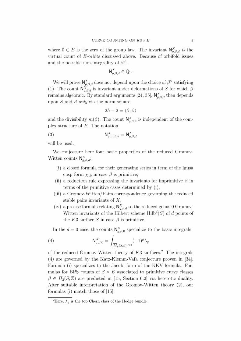
where 0 ∈ E is the zero of the group law. The invariant NXg,β,d is the
virtual count of E-orbits discussed above. Because of orbifold issues
and the possible non-integrality of β∨,
NXg,β,d ∈ Q .
We will prove NXg,β,d does not depend upon the choice of β∨ satisfying
(1). The count NXg,β,d is invariant under deformations of S for which β
remains algebraic. By standard arguments [24, 35], NXg,β,d then depends
upon S and β only via the norm square
2h− 2 = 〈β, β〉
and the divisibility m(β). The count NXg,β,d is independent of the com-
plex structure of E. The notation
(3) NXg,m,h,d = NX
g,β,d
will be used.
We conjecture here four basic properties of the reduced Gromov-
Witten counts NXg,β,d:
(i) a closed formula for their generating series in term of the Igusa
cusp form χ10 in case β is primitive,
(ii) a reduction rule expressing the invariants for imprimitive β in
terms of the primitive cases determined by (i),
(iii) a Gromov-Witten/Pairs correspondence governing the reduced
stable pairs invariants of X ,
(iv) a precise formula relating NXg,β,d to the reduced genus 0 Gromov-
Witten invariants of the Hilbert scheme Hilbd(S) of d points of
the K3 surface S in case β is primitive.
In the d = 0 case, the counts NXg,β,0 specialize to the basic integrals
(4) NXg,β,0 =
∫
[Mg(S,β)]red(−1)gλg
of the reduced Gromov-Witten theory of K3 surfaces.2 The integrals
(4) are governed by the Katz-Klemm-Vafa conjecture proven in [34].
Formula (i) specializes to the Jacobi form of the KKV formula. For-
mulas for BPS counts of S × E associated to primitive curve classes
β ∈ H2(S,Z) are predicted in [15, Section 6.2] via heterotic duality.
After suitable interpretation of the Gromov-Witten theory (2), our
formulas (i) match those of [15].
2Here, λg is the top Chern class of the Hodge bundle.
4 G. OBERDIECK AND R. PANDHARIPANDE
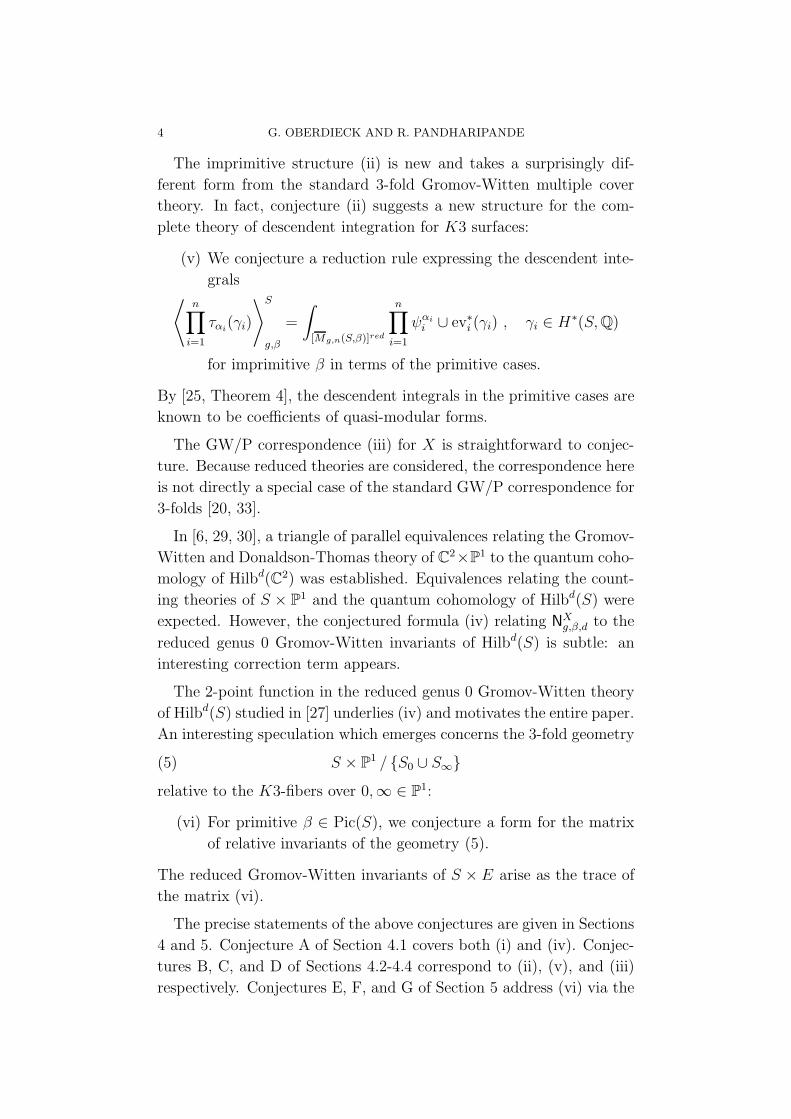
The imprimitive structure (ii) is new and takes a surprisingly dif-
ferent form from the standard 3-fold Gromov-Witten multiple cover
theory. In fact, conjecture (ii) suggests a new structure for the com-
plete theory of descendent integration for K3 surfaces:
(v) We conjecture a reduction rule expressing the descendent inte-
grals⟨
n∏
i=1
ταi(γi)
⟩S
g,β
=
∫
[Mg,n(S,β)]red
n∏
i=1
ψαii ∪ ev∗i (γi) , γi ∈ H
∗(S,Q)
for imprimitive β in terms of the primitive cases.
By [25, Theorem 4], the descendent integrals in the primitive cases are
known to be coefficients of quasi-modular forms.
The GW/P correspondence (iii) for X is straightforward to conjec-
ture. Because reduced theories are considered, the correspondence here
is not directly a special case of the standard GW/P correspondence for
3-folds [20, 33].
In [6, 29, 30], a triangle of parallel equivalences relating the Gromov-
Witten and Donaldson-Thomas theory of C2×P1 to the quantum coho-
mology of Hilbd(C2) was established. Equivalences relating the count-
ing theories of S × P1 and the quantum cohomology of Hilbd(S) were
expected. However, the conjectured formula (iv) relating NXg,β,d to the
reduced genus 0 Gromov-Witten invariants of Hilbd(S) is subtle: an
interesting correction term appears.
The 2-point function in the reduced genus 0 Gromov-Witten theory
of Hilbd(S) studied in [27] underlies (iv) and motivates the entire paper.
An interesting speculation which emerges concerns the 3-fold geometry
(5) S × P1 / S0 ∪ S∞
relative to the K3-fibers over 0,∞ ∈ P1:
(vi) For primitive β ∈ Pic(S), we conjecture a form for the matrix
of relative invariants of the geometry (5).
The reduced Gromov-Witten invariants of S × E arise as the trace of
the matrix (vi).
The precise statements of the above conjectures are given in Sections
4 and 5. Conjecture A of Section 4.1 covers both (i) and (iv). Conjec-
tures B, C, and D of Sections 4.2-4.4 correspond to (ii), (v), and (iii)
respectively. Conjectures E, F, and G of Section 5 address (vi) via the
CURVE COUNTING ON K3× E 5
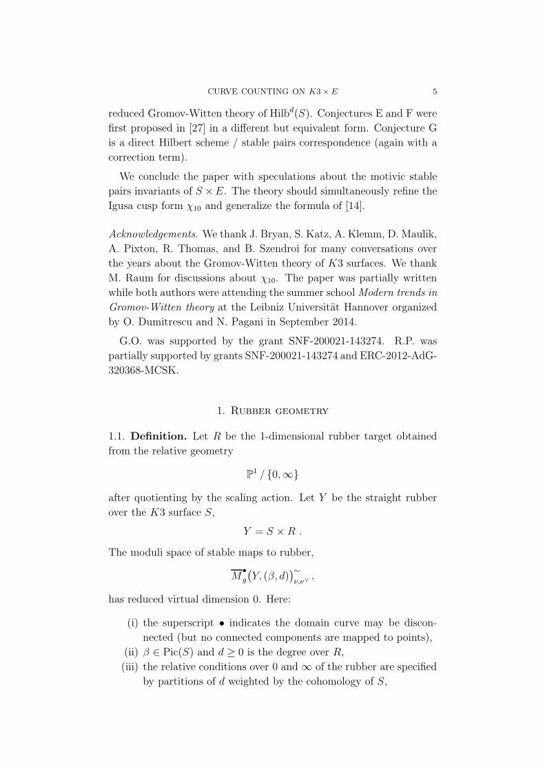
reduced Gromov-Witten theory of Hilbd(S). Conjectures E and F were
first proposed in [27] in a different but equivalent form. Conjecture G
is a direct Hilbert scheme / stable pairs correspondence (again with a
correction term).
We conclude the paper with speculations about the motivic stable
pairs invariants of S ×E. The theory should simultaneously refine the
Igusa cusp form χ10 and generalize the formula of [14].
Acknowledgements. We thank J. Bryan, S. Katz, A. Klemm, D. Maulik,
A. Pixton, R. Thomas, and B. Szendroi for many conversations over
the years about the Gromov-Witten theory of K3 surfaces. We thank
M. Raum for discussions about χ10. The paper was partially written
while both authors were attending the summer school Modern trends in
Gromov-Witten theory at the Leibniz Universitat Hannover organized
by O. Dumitrescu and N. Pagani in September 2014.
G.O. was supported by the grant SNF-200021-143274. R.P. was
partially supported by grants SNF-200021-143274 and ERC-2012-AdG-
320368-MCSK.
1. Rubber geometry
1.1. Definition. Let R be the 1-dimensional rubber target obtained
from the relative geometry
P1 / 0,∞
after quotienting by the scaling action. Let Y be the straight rubber
over the K3 surface S,
Y = S × R .
The moduli space of stable maps to rubber,
M•
g
(Y, (β, d)
)∼ν,ν∨
,
has reduced virtual dimension 0. Here:
(i) the superscript • indicates the domain curve may be discon-
nected (but no connected components are mapped to points),
(ii) β ∈ Pic(S) and d ≥ 0 is the degree over R,
(iii) the relative conditions over 0 and∞ of the rubber are specified
by partitions of d weighted by the cohomology of S,
6 G. OBERDIECK AND R. PANDHARIPANDE
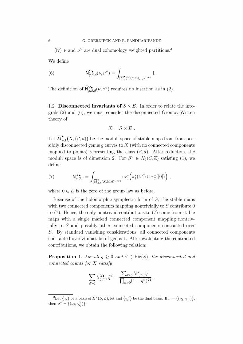
(iv) ν and ν∨ are dual cohomology weighted partitions.3
We define
(6) NY •g,β,d(ν, ν
∨) =
∫
[M•
g(Y,(β,d))ν,ν∨ ]red1 .
The definition of NY •g,β,d(ν, ν
∨) requires no insertion as in (2).
1.2. Disconnected invariants of S ×E. In order to relate the inte-
grals (2) and (6), we must consider the disconnected Gromov-Witten
theory of
X = S ×E .
Let M•
g,1
(X, (β, d)
)be the moduli space of stable maps from from pos-
sibily disconnected genus g curves toX (with no connected components
mapped to points) representing the class (β, d). After reduction, the
moduli space is of dimension 2. For β∨ ∈ H2(S,Z) satisfing (1), we
define
(7) NX•g,β,d =
∫
[M•
g,1(X,(β,d))]redev∗1
(π∗1(β
∨) ∪ π∗2([0])
),
where 0 ∈ E is the zero of the group law as before.
Because of the holomorphic symplectic form of S, the stable maps
with two connected components mapping nontrivially to S contribute 0
to (7). Hence, the only nontrivial contibutions to (7) come from stable
maps with a single marked connected component mapping nontriv-
ially to S and possibly other connected components contracted over
S. By standard vanishing considerations, all connected components
contracted over S must be of genus 1. After evaluating the contracted
contributions, we obtain the following relation:
Proposition 1. For all g ≥ 0 and β ∈ Pic(S), the disconnected and
connected counts for X satisfy
∑
d≥0
NX•g,β,d q
d =
∑d≥0 N
Xg,β,d q
d
∏n>0(1− q
n)24.
3Let γi be a basis ofH∗(S,Z), let and γ∨
i be the dual basis. If ν = (νj, γij ),
then ν∨ = (νj , γ∨
ij).
CURVE COUNTING ON K3× E 7
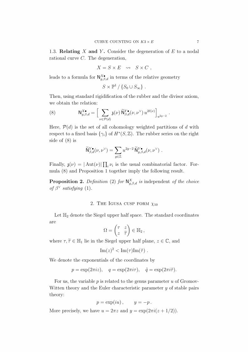
1.3. Relating X and Y . Consider the degeneration of E to a nodal
rational curve C. The degeneration,
X = S ×E S × C ,
leads to a formula for NX•g,β,d in terms of the relative geometry
S × P1 / S0 ∪ S∞ .
Then, using standard rigidification of the rubber and the divisor axiom,
we obtain the relation:
(8) NX•g,β,d =
[ ∑
ν∈P(d)
z(ν) NY •β,d(ν, ν
∨) u2ℓ(ν)]u2g−2
.
Here, P(d) is the set of all cohomology weighted partitions of d with
respect to a fixed basis γi of H∗(S,Z). The rubber series on the right
side of (8) is
NY •β,d(ν, ν
∨) =∑
g∈Z
u2g−2 NY •g,β,d(ν, ν
∨) .
Finally, z(ν) = |Aut(ν)|∏
i νi is the usual combinatorial factor. For-
mula (8) and Proposition 1 together imply the following result.
Proposition 2. Definition (2) for NXg,β,d is independent of the choice
of β∨ satisfying (1).
2. The Igusa cusp form χ10
Let H2 denote the Siegel upper half space. The standard coordinates
are
Ω =
(τ zz τ
)∈ H2 ,
where τ, τ ∈ H1 lie in the Siegel upper half plane, z ∈ C, and
Im(z)2 < Im(τ)Im(τ ) .
We denote the exponentials of the coordinates by
p = exp(2πiz), q = exp(2πiτ), q = exp(2πiτ).
For us, the variable p is related to the genus parameter u of Gromov-
Witten theory and the Euler characteristic parameter y of stable pairs
theory:
p = exp(iu) , y = −p .
More precisely, we have u = 2πz and y = exp(2πi(z + 1/2)).
8 G. OBERDIECK AND R. PANDHARIPANDE
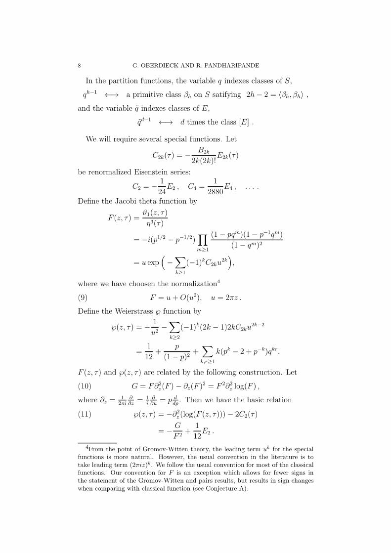
In the partition functions, the variable q indexes classes of S,
qh−1 ←→ a primitive class βh on S satifying 2h− 2 = 〈βh, βh〉 ,
and the variable q indexes classes of E,
qd−1 ←→ d times the class [E] .
We will require several special functions. Let
C2k(τ) = −B2k
2k(2k)!E2k(τ)
be renormalized Eisenstein series:
C2 = −1
24E2 , C4 =
1
2880E4 , . . . .
Define the Jacobi theta function by
F (z, τ) =ϑ1(z, τ)
η3(τ)
= −i(p1/2 − p−1/2)∏
m≥1
(1− pqm)(1− p−1qm)
(1− qm)2
= u exp(−∑
k≥1
(−1)kC2ku2k),
where we have choosen the normalization4
(9) F = u+O(u2), u = 2πz .
Define the Weierstrass ℘ function by
℘(z, τ) = −1
u2−∑
k≥2
(−1)k(2k − 1)2kC2ku2k−2
=1
12+
p
(1− p)2+∑
k,r≥1
k(pk − 2 + p−k)qkr.
F (z, τ) and ℘(z, τ) are related by the following construction. Let
(10) G = F∂2z (F )− ∂z(F )2 = F 2∂2z log(F ) ,
where ∂z =1
2πi∂∂z
= 1i
∂∂u
= p ddp. Then we have the basic relation
℘(z, τ) = −∂2z (log(F (z, τ)))− 2C2(τ)(11)
= −G
F 2+
1
12E2 .
4From the point of Gromov-Witten theory, the leading term uk for the specialfunctions is more natural. However, the usual convention in the literature is totake leading term (2πiz)k. We follow the usual convention for most of the classicalfunctions. Our convention for F is an exception which allows for fewer signs inthe statement of the Gromov-Witten and pairs results, but results in sign changeswhen comparing with classical function (see Conjecture A).
CURVE COUNTING ON K3× E 9
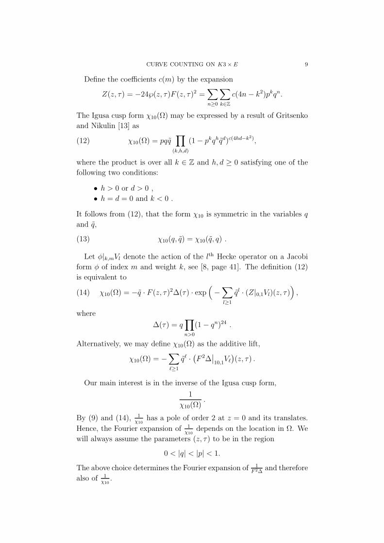
Define the coefficients c(m) by the expansion
Z(z, τ) = −24℘(z, τ)F (z, τ)2 =∑
n≥0
∑
k∈Z
c(4n− k2)pkqn.
The Igusa cusp form χ10(Ω) may be expressed by a result of Gritsenko
and Nikulin [13] as
(12) χ10(Ω) = pqq∏
(k,h,d)
(1− pkqhqd)c(4hd−k2),
where the product is over all k ∈ Z and h, d ≥ 0 satisfying one of the
following two conditions:
• h > 0 or d > 0 ,
• h = d = 0 and k < 0 .
It follows from (12), that the form χ10 is symmetric in the variables q
and q,
(13) χ10(q, q) = χ10(q, q) .
Let φ|k,mVl denote the action of the lth Hecke operator on a Jacobi
form φ of index m and weight k, see [8, page 41]. The definition (12)
is equivalent to
(14) χ10(Ω) = −q · F (z, τ)2∆(τ) · exp
(−∑
l≥1
ql · (Z|0,1Vl)(z, τ)),
where
∆(τ) = q∏
n>0
(1− qn)24 .
Alternatively, we may define χ10(Ω) as the additive lift,
χ10(Ω) = −∑
ℓ≥1
qℓ ·(F 2∆
∣∣10,1
Vℓ)(z, τ) .
Our main interest is in the inverse of the Igusa cusp form,
1
χ10(Ω).
By (9) and (14), 1χ10
has a pole of order 2 at z = 0 and its translates.
Hence, the Fourier expansion of 1χ10
depends on the location in Ω. We
will always assume the parameters (z, τ) to be in the region
0 < |q| < |p| < 1.
The above choice determines the Fourier expansion of 1F 2∆
and therefore
also of 1χ10
.
10 G. OBERDIECK AND R. PANDHARIPANDE
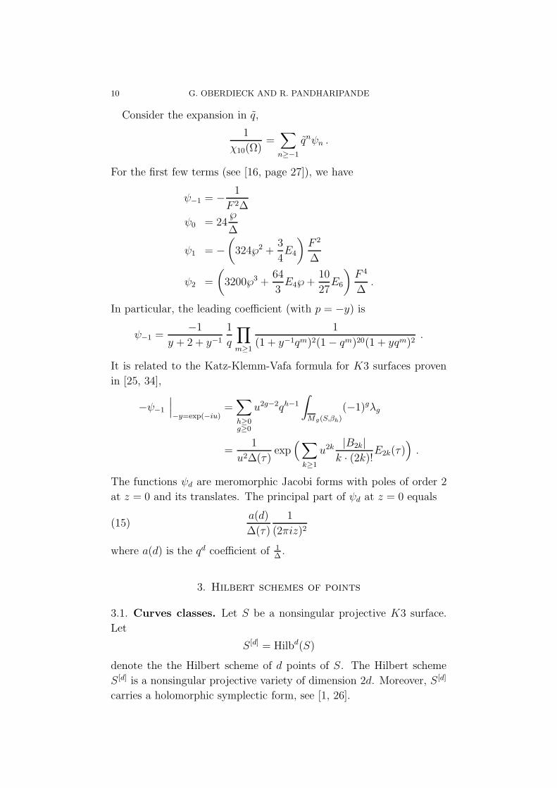
Consider the expansion in q,
1
χ10(Ω)=∑
n≥−1
qnψn .
For the first few terms (see [16, page 27]), we have
ψ−1 = −1
F 2∆
ψ0 = 24℘
∆
ψ1 = −
(324℘2 +
3
4E4
)F 2
∆
ψ2 =
(3200℘3 +
64
3E4℘+
10
27E6
)F 4
∆.
In particular, the leading coefficient (with p = −y) is
ψ−1 =−1
y + 2 + y−1
1
q
∏
m≥1
1
(1 + y−1qm)2(1− qm)20(1 + yqm)2.
It is related to the Katz-Klemm-Vafa formula for K3 surfaces proven
in [25, 34],
−ψ−1
∣∣∣−y=exp(−iu)
=∑
h≥0g≥0
u2g−2qh−1
∫
Mg(S,βh)
(−1)gλg
=1
u2∆(τ)exp
(∑
k≥1
u2k|B2k|
k · (2k)!E2k(τ)
).
The functions ψd are meromorphic Jacobi forms with poles of order 2
at z = 0 and its translates. The principal part of ψd at z = 0 equals
(15)a(d)
∆(τ)
1
(2πiz)2
where a(d) is the qd coefficient of 1∆.
3. Hilbert schemes of points
3.1. Curves classes. Let S be a nonsingular projective K3 surface.
Let
S [d] = Hilbd(S)
denote the the Hilbert scheme of d points of S. The Hilbert scheme
S [d] is a nonsingular projective variety of dimension 2d. Moreover, S [d]
carries a holomorphic symplectic form, see [1, 26].
CURVE COUNTING ON K3× E 11
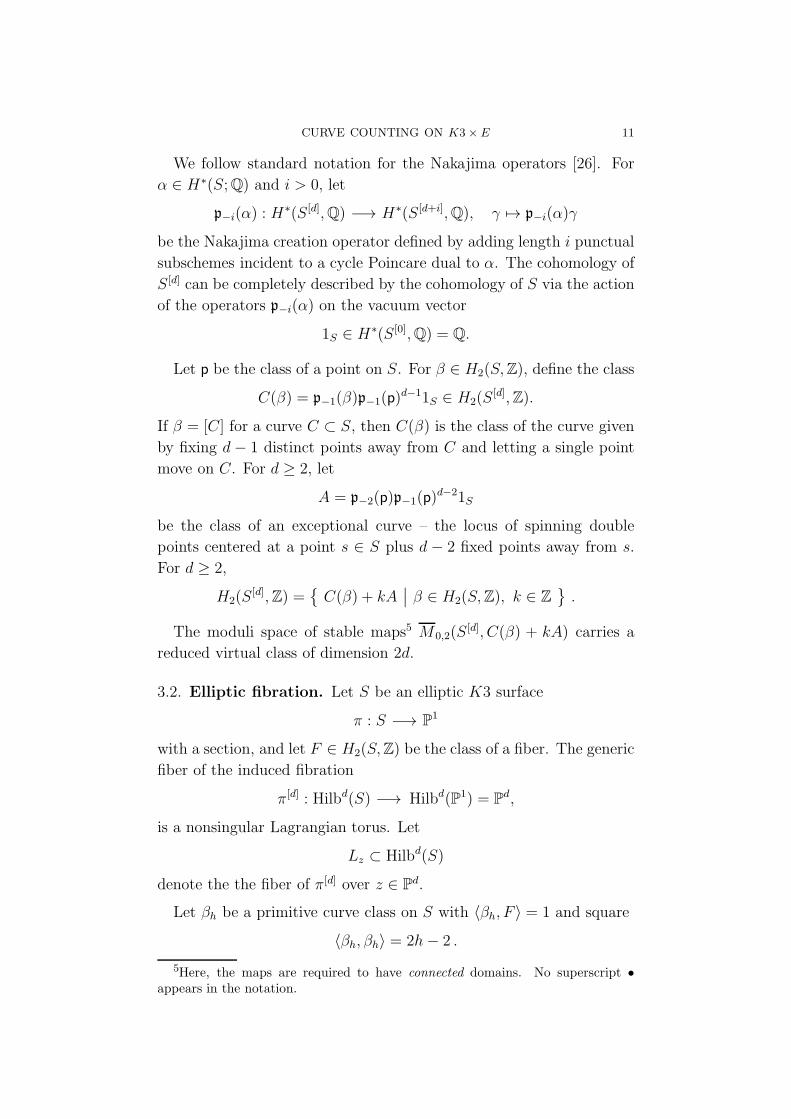
We follow standard notation for the Nakajima operators [26]. For
α ∈ H∗(S;Q) and i > 0, let
p−i(α) : H∗(S [d],Q) −→ H∗(S [d+i],Q), γ 7→ p−i(α)γ
be the Nakajima creation operator defined by adding length i punctual
subschemes incident to a cycle Poincare dual to α. The cohomology of
S [d] can be completely described by the cohomology of S via the action
of the operators p−i(α) on the vacuum vector
1S ∈ H∗(S [0],Q) = Q.
Let p be the class of a point on S. For β ∈ H2(S,Z), define the class
C(β) = p−1(β)p−1(p)d−11S ∈ H2(S
[d],Z).
If β = [C] for a curve C ⊂ S, then C(β) is the class of the curve given
by fixing d − 1 distinct points away from C and letting a single point
move on C. For d ≥ 2, let
A = p−2(p)p−1(p)d−21S
be the class of an exceptional curve – the locus of spinning double
points centered at a point s ∈ S plus d − 2 fixed points away from s.
For d ≥ 2,
H2(S[d],Z) =
C(β) + kA
∣∣ β ∈ H2(S,Z), k ∈ Z.
The moduli space of stable maps5 M 0,2(S[d], C(β) + kA) carries a
reduced virtual class of dimension 2d.
3.2. Elliptic fibration. Let S be an elliptic K3 surface
π : S −→ P1
with a section, and let F ∈ H2(S,Z) be the class of a fiber. The generic
fiber of the induced fibration
π[d] : Hilbd(S) −→ Hilbd(P1) = Pd,
is a nonsingular Lagrangian torus. Let
Lz ⊂ Hilbd(S)
denote the the fiber of π[d] over z ∈ Pd.
Let βh be a primitive curve class on S with 〈βh, F 〉 = 1 and square
〈βh, βh〉 = 2h− 2 .
5Here, the maps are required to have connected domains. No superscript •appears in the notation.
12 G. OBERDIECK AND R. PANDHARIPANDE
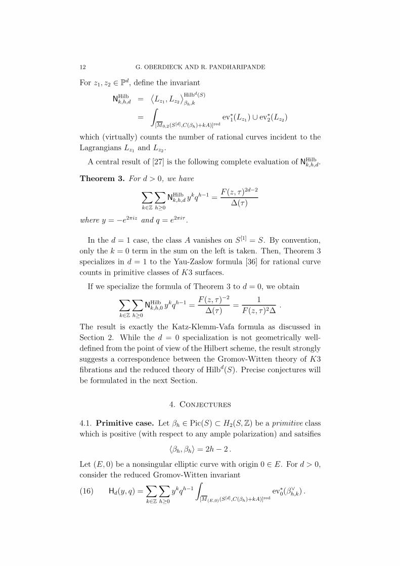
For z1, z2 ∈ Pd, define the invariant
NHilbk,h,d =
⟨Lz1 , Lz2
⟩Hilbd(S)
βh,k
=
∫
[M0,2(S[d],C(βh)+kA)]redev∗1(Lz1) ∪ ev∗2(Lz2)
which (virtually) counts the number of rational curves incident to the
Lagrangians Lz1 and Lz2 .
A central result of [27] is the following complete evaluation of NHilbk,h,d.
Theorem 3. For d > 0, we have
∑
k∈Z
∑
h≥0
NHilbk,h,d y
kqh−1 =F (z, τ)2d−2
∆(τ)
where y = −e2πiz and q = e2πiτ .
In the d = 1 case, the class A vanishes on S [1] = S. By convention,
only the k = 0 term in the sum on the left is taken. Then, Theorem 3
specializes in d = 1 to the Yau-Zaslow formula [36] for rational curve
counts in primitive classes of K3 surfaces.
If we specialize the formula of Theorem 3 to d = 0, we obtain
∑
k∈Z
∑
h≥0
NHilbk,h,0 y
kqh−1 =F (z, τ)−2
∆(τ)=
1
F (z, τ)2∆.
The result is exactly the Katz-Klemm-Vafa formula as discussed in
Section 2. While the d = 0 specialization is not geometrically well-
defined from the point of view of the Hilbert scheme, the result strongly
suggests a correspondence between the Gromov-Witten theory of K3
fibrations and the reduced theory of Hilbd(S). Precise conjectures will
be formulated in the next Section.
4. Conjectures
4.1. Primitive case. Let βh ∈ Pic(S) ⊂ H2(S,Z) be a primitive class
which is positive (with respect to any ample polarization) and satsifies
〈βh, βh〉 = 2h− 2 .
Let (E, 0) be a nonsingular elliptic curve with origin 0 ∈ E. For d > 0,
consider the reduced Gromov-Witten invariant
(16) Hd(y, q) =∑
k∈Z
∑
h≥0
ykqh−1
∫
[M(E,0)(S[d],C(βh)+kA)]redev∗0(β
∨h,k) .
CURVE COUNTING ON K3× E 13
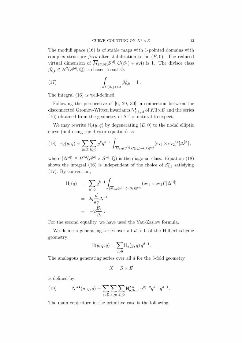
The moduli space (16) is of stable maps with 1-pointed domains with
complex structure fixed after stabilization to be (E, 0). The reduced
virtual dimension of M (E,0)(S[d], C(βh) + kA) is 1. The divisor class
β∨h,k ∈ H
2(S [d],Q) is chosen to satisfy
(17)
∫
C(βh)+kA
β∨h,k = 1 .
The integral (16) is well-defined.
Following the perspective of [6, 29, 30], a connection between the
disconnected Gromov-Witten invariants N•g,βh,d
ofK3×E and the series
(16) obtained from the geometry of S [d] is natural to expect.
We may rewrite Hd(y, q) by degenerating (E, 0) to the nodal elliptic
curve (and using the divisor equation) as
(18) Hd(y, q) =∑
k∈Z
∑
h≥0
ykqh−1
∫
[M0,2(S[d],C(βh)+kA)]red(ev1× ev2)
∗[∆[d]] ,
where [∆[d]] ∈ H2d(S [d] × S [d],Q) is the diagonal class. Equation (18)
shows the integral (16) is independent of the choice of β∨h,k satisfying
(17). By convention,
H1(q) =∑
h≥0
qh−1
∫
[M0,2(S[1],C(βh))]red(ev1× ev2)
∗[∆[1]]
= 2qd
dq∆−1
= −2E2
∆.
For the second equality, we have used the Yau-Zaslow formula.
We define a generating series over all d > 0 of the Hilbert scheme
geometry:
H(y, q, q) =∑
d>0
Hd(y, q) qd−1.
The analogous generating series over all d for the 3-fold geometry
X = S × E
is defined by
(19) NX•(u, q, q) =∑
g∈Z
∑
h≥0
∑
d≥0
NX•g,βh,d
u2g−2qh−1qd−1.
The main conjecture in the primitive case is the following.
14 G. OBERDIECK AND R. PANDHARIPANDE
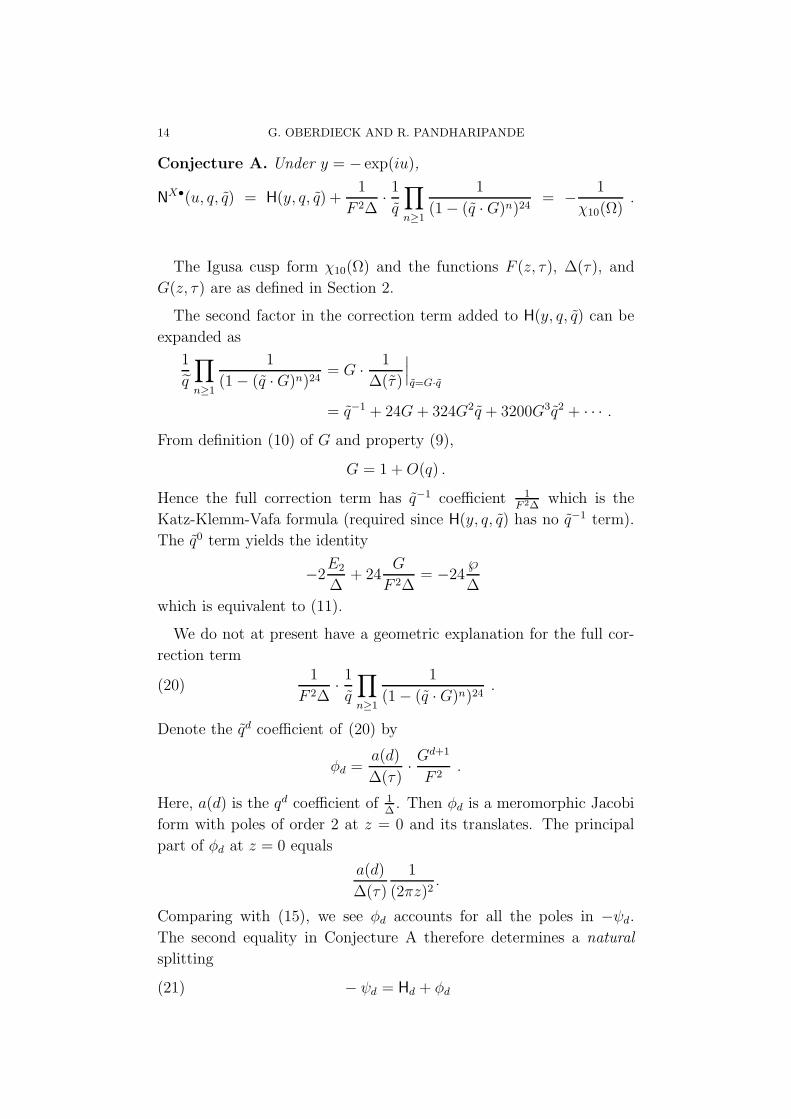
Conjecture A. Under y = − exp(iu),
NX•(u, q, q) = H(y, q, q) +1
F 2∆·1
q
∏
n≥1
1
(1− (q ·G)n)24= −
1
χ10(Ω).
The Igusa cusp form χ10(Ω) and the functions F (z, τ), ∆(τ), and
G(z, τ) are as defined in Section 2.
The second factor in the correction term added to H(y, q, q) can be
expanded as
1
q
∏
n≥1
1
(1− (q ·G)n)24= G ·
1
∆(τ )
∣∣∣q=G·q
= q−1 + 24G+ 324G2q + 3200G3q2 + · · · .
From definition (10) of G and property (9),
G = 1 +O(q) .
Hence the full correction term has q−1 coefficient 1F 2∆
which is the
Katz-Klemm-Vafa formula (required since H(y, q, q) has no q−1 term).
The q0 term yields the identity
−2E2
∆+ 24
G
F 2∆= −24
℘
∆
which is equivalent to (11).
We do not at present have a geometric explanation for the full cor-
rection term
(20)1
F 2∆·1
q
∏
n≥1
1
(1− (q ·G)n)24.
Denote the qd coefficient of (20) by
φd =a(d)
∆(τ)·Gd+1
F 2.
Here, a(d) is the qd coefficient of 1∆. Then φd is a meromorphic Jacobi
form with poles of order 2 at z = 0 and its translates. The principal
part of φd at z = 0 equals
a(d)
∆(τ)
1
(2πz)2.
Comparing with (15), we see φd accounts for all the poles in −ψd.
The second equality in Conjecture A therefore determines a natural
splitting
(21) − ψd = Hd + φd
CURVE COUNTING ON K3× E 15
of −ψd into a finite (holomorphic) quasi-Jacobi form Hd and a polar
part φd. In particular, the Fourier expansion of Hd is independent of the
moduli τ . Hence, all wall-crossings are related to φd. The splitting of
ψd into a finite and polar part has been studied by Dabholkar, Murthy,
and Zagier [7] and has a direct interpretation in a physical model of
quantum black holes. In fact, up to the E2 summand in (11) our
splitting matches their simplest choice, see [7, Equations 1.5 and 9.1].
The two equalities of Conjecture A are independent claims. The first
is a correspondence result (up to correction). We have made verifica-
tions by partially evaluating both sides. The second equality, which
evalutes the series, has already been seen to hold for the coefficients of
q−1 and q0. The second equality has been proven for the coefficient of
q1 in [27]. The conjecture
(22) NX•(u, q, q) = −1
χ10(Ω)
is directly related to the predictions of Section 6.2 of [15]. J. Bryan [4]
has verified6 conjecture (22) for the coefficients q−1 and q0.
The conjectural equality (22) may be viewed as a mathematically
precise formulation of [15, Section 6.2]. The Igusa cusp form χ10 ap-
pears in [15] via the elliptic genera of the symmetric products of a K3
surface (the χ10 terminology is not used in [15]). The development of
the reduced virtual class occurred in the years following [15]. Since
the K3 × E geometry carries a free E-action, a further step (beyond
reduction) must be taken to avoid a trivial theory. Definition (2) with
an insertion is a straightforward solution. Finally, the Igusa cusp form
χ10 is related to the disconnected reduced Gromov-Witten theory of
K3 × E. With these foundations, the prediction of [15] may be inter-
preted to exactly match (22).
By the symmetry (13) of the Igusa cusp form χ10, Conjecture A
predicts a surprising symmetry for disconnected Gromov-Witten theory
of X ,
NX•g,βh,d
= NX•g,βd,h
,
for all primitive classes βh and βd. In the notation (3), the symmetry
can be written as
NX•g,1,h,d = NX•
g,1,d,h
for all h, d ≥ 0 (where the subscript 1 denotes primitivity).
6Bryan’s calculation is on the sheaf theory side, see Conjecture D below.
16 G. OBERDIECK AND R. PANDHARIPANDE
Conjectures for the motivic generalization of the d = 0 case are
presented in [14]. An interesting connection to the Mathieu M24 moon-
shine phenomena appears there in the data. Since the Gromov-Witten
theory of X is related via − 1χ10
by Conjecture A to the elliptic genera
of the symmetric products of K3 surfaces, the Mathieu M24 moonshine
must also arise here.
4.2. Imprimitive classes. The generating series NX•(u, q, q) defined
by (19) concerns only the primitive classes βh ∈ Pic(S). To study the
imprimitive case, we define
(23) NXβ (u, q) =
∑
g∈Z
∑
d≥0
NXg,β,d u
2g−2qd−1
for any β ∈ Pic(S). The coefficents of NXβ (u, q) are connected invari-
ants.7 We may write (23) in the notation (3) as
NXmβh
(u, q) =∑
g≥0
∑
d≥0
NXg,m,m2(h−1)+1,d u
2g−2qd−1
for primitive βh ∈ Pic(S) satisfying
〈βh, βh〉 = 2h− 2 .
In the primitive (m=1) case, instead of writing NXβh, we write
NXh (u, q) =
∑
g≥0
∑
d≥0
NXg,1,h,d u
2g−2qd−1
Conjecture B. For all m > 0,
(24) NXmβh
(u, q) =∑
k|m
1
kNX
(mk)2(h−1)+1(ku, q) ,
for the primitive class βh.
Conjecture B expresses the series NXmβh
in terms of series for primitive
classes corresponding to the divisors k of m. To such a divisor k, we
associate the class mkβh with square
⟨mkβh,
m
kβh
⟩=(mk
)2(2h− 2) = 2
((mk
)2(h− 1) + 1
)− 2 .
The term in the sum on the right side of (24) corresponding to k
may be viewed as the contribution of the primitive class of square
7By Proposition 1, there is no difficulty in moving back and forth between con-nected and disconnected invariants.
CURVE COUNTING ON K3× E 17
equal to 〈mkβh,
mkβh〉. The primitive contribution of the divisor k to
NXg,m,m2(h−1)+1,d is
(25) k2g−3 · NX
g,1,(mk )
2(h−1)+1,d
.
The scaling factor k2g−3 is independent of d. In fact, the variable q
plays no role in formula (24). To emphasize the point, the contribution
of the divisor k geometrically is a contribution of the class(mkβh, d
)= ιS∗
(mkβ)+ ιE∗(d[E])
to (mβh, d) in the 3-fold S ×E. Unless d = 0, such a contribution can
not be viewed as a multiple cover contribution in the usual Gopakumar-
Vafa perspective of Calabi-Yau 3-fold invariants.
In the d = 0 case, Conjecture B specializes to the multiple cover
structure of the KKV conjecture proven in [34] which is usually formu-
lated in terms of BPS counts. We could rewrite Conjecture B in terms
of nonstandard 3-fold BPS counts which do not interact with the curve
class [E] associated to q. Instead, we have written Conjecture B in the
most straightforward Gromov-Witten form. In fact, the simple form
of Conjecture B suggests a much more general underlying structure for
K3 surfaces (which we will discuss in Section 4.3).
Further evidence for Conjecture B can be found in case h = 0. Lo-
calization arguments8 (with respect to the C∗ acting on the −2 curve)
yield
NXmβ0
(u, q) =1
mNX
0 (mu, q) .
Hence, Conjecture B predicts the primitive contributions corresponding
to k 6= m all vanish in the h = 0 case. Such vanishing is correct: the
reduced Gromov-Witten invariants of X vanish for classes (β, d) where
β is primitive and
〈β, β〉 < −2 .
Finally, an elementary analysis leads to the proof of Conjecture B in
all cases for g = 1. Both sides of (24) are easily calculated.
4.3. Descendent theory for K3 surfaces. Let S be a nonsingular
projective K3 surface, and let β ∈ Pic(S) be a positive class. We define
8The localization required here is parallel to the proof of the scaling in [9, The-orem 3].
18 G. OBERDIECK AND R. PANDHARIPANDE
the (reduced) descendent Gromov-Witten invariants by⟨
n∏
i=1
ταi(γi)
⟩S
g,β
=
∫
[Mg,n(S,β)]red
n∏
i=1
ψαii ∪ ev∗i (γi) , γi ∈ H
∗(S,Q) .
A potential function for the descendent theory of K3 surfaces in prim-
itive classes is defined by
(26) Fg
(τk1(γl1) · · · τkr(γlr)
)=
∞∑
h=0
⟨τk1(γl1) · · · τkr(γlr)
⟩Sg,βh
qh−1
for g ≥ 0.
The descendent potential (26) is a quasimodular form [25]. The ring
QMod = Q[E2(q), E4(q), E6(q)]
of holomorphic quasimodular forms (of level 1) is the Q-algebra gen-
erated by Eisenstein series E2k, see [3]. The ring QMod is naturally
graded by weight (where E2k has weight 2k) and inherits an increasing
filtration
QMod≤2k ⊂ QMod
given by forms of weight ≤ 2k. The precise result proven in [25] is the
following.
Theorem 4. The descendent potential is the Fourier expansion in q of
a quasimodular form
Fg(τk1(γ1) · · · τkr(γr)) ∈1
∆(q)QMod≤2g+2r
with pole at q = 0 of order at most 1.
Conjectures C1 and C2 below will reduce all descendent invariants to
the primitive case.
Conjecture C1 is an invariance property. Let S and S be two K3
surfaces, and let
ϕ :(H2(S,R) , 〈, 〉
)→(H2(S ,R), 〈, 〉
)
be a real isometry sending a effective curve9 class β ∈ H2(S,Z) to an
effective curve class β ∈ H2(S,Z),
ϕ(β) = β .
9Since there is a canonical isomorphism H2(S,Z)∼
= H2(S,Z) , we may considerβ also as a cohomology class.
CURVE COUNTING ON K3× E 19
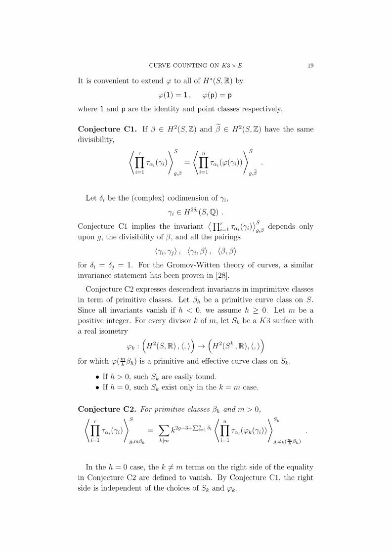
It is convenient to extend ϕ to all of H∗(S,R) by
ϕ(1) = 1 , ϕ(p) = p
where 1 and p are the identity and point classes respectively.
Conjecture C1. If β ∈ H2(S,Z) and β ∈ H2(S,Z) have the same
divisibility,⟨
r∏
i=1
ταi(γi)
⟩S
g,β
=
⟨n∏
i=1
ταi(ϕ(γi))
⟩S
g,β
.
Let δi be the (complex) codimension of γi,
γi ∈ H2δi(S,Q) .
Conjecture C1 implies the invariant⟨∏r
i=1 ταi(γi)⟩Sg,β
depends only
upon g, the divisibility of β, and all the pairings
〈γi, γj〉 , 〈γi, β〉 , 〈β, β〉
for δi = δj = 1. For the Gromov-Witten theory of curves, a similar
invariance statement has been proven in [28].
Conjecture C2 expresses descendent invariants in imprimitive classes
in term of primitive classes. Let βh be a primitive curve class on S.
Since all invariants vanish if h < 0, we assume h ≥ 0. Let m be a
positive integer. For every divisor k of m, let Sk be a K3 surface with
a real isometry
ϕk :(H2(S,R) , 〈, 〉
)→(H2(Sk ,R), 〈, 〉
)
for which ϕ(mkβh) is a primitive and effective curve class on Sk.
• If h > 0, such Sk are easily found.
• If h = 0, such Sk exist only in the k = m case.
Conjecture C2. For primitive classes βh and m > 0,⟨
r∏
i=1
ταi(γi)
⟩S
g,mβh
=∑
k|m
k2g−3+∑n
i=1 δi
⟨n∏
i=1
ταi(ϕk(γi))
⟩Sk
g,ϕk(mkβh)
.
In the h = 0 case, the k 6= m terms on the right side of the equality
in Conjecture C2 are defined to vanish. By Conjecture C1, the right
side is independent of the choices of Sk and ϕk.
20 G. OBERDIECK AND R. PANDHARIPANDE
The first evidence: the KKV formula interpreted as the Hodge inte-
gral (4) exactly satisfies Conjecture C2 with the integrand viewed as
having no descendent insertions. In fact, (−1)gλg can be expanded in
terms of descendent integrands on strata — applying Conjecture C2 to
such an expansion exactly yields the multiple cover scaling of the KKV
formula. In particular, Conjecture C2 together with the KKV formula
in the primitive case implies the full KKV formula.
Conjecture B, when fully expanded, has a scaling factor of k2g−3
which corresponds to Conjecture C2 with no insertions. In fact, Con-
jecture B follows from Conjecture C2 via the product formula [2] for
virtual classes in Gromov-Witten theory. Conjecture C2 was motived
for us by Conjecture B.
The second evidence: Maulik in [21, Theorem 1.1] calculated descen-
dents for the A1 singularity. We may interpret the calculation of [21] as
verifiying Conjecture C2 in case h = 0. The scaling of Conjecture C2
appears in [21, Theorem 1.1] as the final result because the primitive
contributions corresponding to k 6= m all vanish in the h = 0 case. Of
course, the A1 singularity only captures codimensions 0 and 1 for δ.
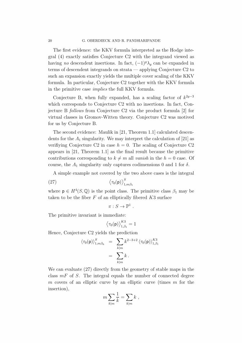
A simple example not covered by the two above cases is the integral
(27)⟨τ0(p)
⟩S1,mβ1
where p ∈ H4(S,Q) is the point class. The primitive class β1 may be
taken to be the fiber F of an elliptically fibered K3 surface
π : S → P1 .
The primitive invariant is immediate:⟨τ0(p)
⟩K3
1,β1= 1
Hence, Conjecture C2 yields the prediction
〈τ0(p)〉S1,mβh
=∑
k|m
k2−3+2 〈τ0(p)〉K31,β1
=∑
k|m
k .
We can evaluate (27) directly from the geometry of stable maps in the
class mF of S. The integral equals the number of connected degree
m covers of an elliptic curve by an elliptic curve (times m for the
insertion),
m∑
k|m
1
k=∑
k|m
k ,
CURVE COUNTING ON K3× E 21
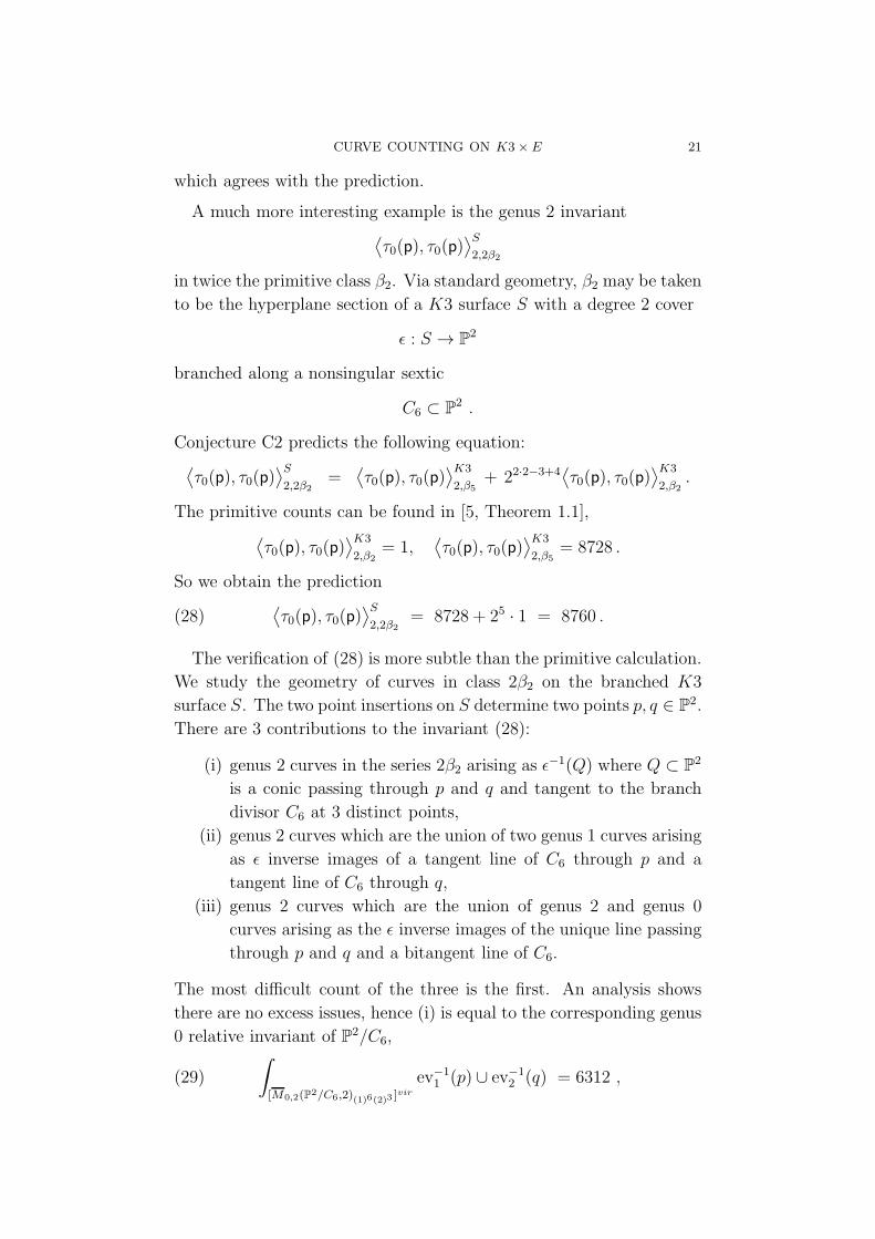
which agrees with the prediction.
A much more interesting example is the genus 2 invariant⟨τ0(p), τ0(p)
⟩S2,2β2
in twice the primitive class β2. Via standard geometry, β2 may be taken
to be the hyperplane section of a K3 surface S with a degree 2 cover
ǫ : S → P2
branched along a nonsingular sextic
C6 ⊂ P2 .
Conjecture C2 predicts the following equation:⟨τ0(p), τ0(p)
⟩S2,2β2
=⟨τ0(p), τ0(p)
⟩K3
2,β5+ 22·2−3+4
⟨τ0(p), τ0(p)
⟩K3
2,β2.
The primitive counts can be found in [5, Theorem 1.1],⟨τ0(p), τ0(p)
⟩K3
2,β2= 1,
⟨τ0(p), τ0(p)
⟩K3
2,β5= 8728 .
So we obtain the prediction
(28)⟨τ0(p), τ0(p)
⟩S2,2β2
= 8728 + 25 · 1 = 8760 .
The verification of (28) is more subtle than the primitive calculation.
We study the geometry of curves in class 2β2 on the branched K3
surface S. The two point insertions on S determine two points p, q ∈ P2.
There are 3 contributions to the invariant (28):
(i) genus 2 curves in the series 2β2 arising as ǫ−1(Q) where Q ⊂ P2
is a conic passing through p and q and tangent to the branch
divisor C6 at 3 distinct points,
(ii) genus 2 curves which are the union of two genus 1 curves arising
as ǫ inverse images of a tangent line of C6 through p and a
tangent line of C6 through q,
(iii) genus 2 curves which are the union of genus 2 and genus 0
curves arising as the ǫ inverse images of the unique line passing
through p and q and a bitangent line of C6.
The most difficult count of the three is the first. An analysis shows
there are no excess issues, hence (i) is equal to the corresponding genus
0 relative invariant of P2/C6,
(29)
∫
[M0,2(P2/C6,2)(1)6(2)3 ]vir
ev−11 (p) ∪ ev−1
2 (q) = 6312 ,
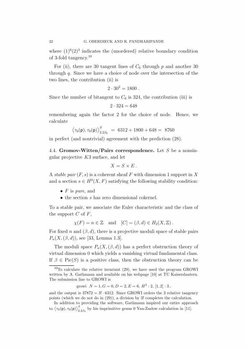
22 G. OBERDIECK AND R. PANDHARIPANDE
where (1)6(2)3 indicates the (unordered) relative boundary condition
of 3-fold tangency.10
For (ii), there are 30 tangent lines of C6 through p and another 30
through q. Since we have a choice of node over the intersection of the
two lines, the contribution (ii) is
2 · 302 = 1800 .
Since the number of bitangent to C6 is 324, the contribution (iii) is
2 · 324 = 648
remembering again the factor 2 for the choice of node. Hence, we
calculate⟨τ0(p), τ0(p)
⟩S2,2β2
= 6312 + 1800 + 648 = 8760
in perfect (and nontrivial) agreement with the prediction (28).
4.4. Gromov-Witten/Pairs correspondence. Let S be a nonsin-
gular projective K3 surface, and let
X = S ×E .
A stable pair (F, s) is a coherent sheaf F with dimension 1 support in X
and a section s ∈ H0(X,F ) satisfying the following stability condition:
• F is pure, and
• the section s has zero dimensional cokernel.
To a stable pair, we associate the Euler characteristic and the class of
the support C of F ,
χ(F ) = n ∈ Z and [C] = (β, d) ∈ H2(X,Z) .
For fixed n and (β, d), there is a projective moduli space of stable pairs
Pn(X, (β, d)), see [33, Lemma 1.3].
The moduli space Pn(X, (β, d)) has a perfect obstruction theory of
virtual dimension 0 which yields a vanishing virtual fundamental class.
If β ∈ Pic(S) is a positive class, then the obstruction theory can be
10To calculate the relative invariant (29), we have used the program GROWIwritten by A. Gathmann and available on his webpage [10] at TU Kaiserslautern.The submission line to GROWI is
growi N = 1, G = 0, D = 2, E = 6, H2 : 2, [1, 2] : 3 ,
and the output is 37872 = 3! · 6312. Since GROWI orders the 3 relative tangencypoints (which we do not do in (29)), a division by 3! completes the calculation.
In addition to providing the software, Gathmann inspired our entire approach
to⟨τ0(p), τ0(p)
⟩S2,2β2
by his imprimitive genus 0 Yau-Zaslow calculation in [11].
CURVE COUNTING ON K3× E 23
reduced to obtain virtual dimension 1. Let β∨ ∈ H2(S,Q) be any class
satisfying
(30) 〈β, β∨〉 = 1
with respect to the intersection pairing on S. For n ∈ Z, we define
(31) PXn,β,d =
∫
[Pn(X,(β,d))]redτ0
(π∗1(β
∨) ∪ π∗2([0])
).
We follow here the notation of Section 0 for the projections π1 and
π2. The insertions in stable pairs theory are defined in [33]. Definition
(31) is parallel to (2). As in the Gromov-Witten case, definition (31)
is independent of β∨ satisfying (30) by degeneration and the study of
the stable pairs theory of the rubber geometry Y .
Define the generating series of stable pairs invariants for X is class
(β, d) by
PXβ,d(y) =
∑
n∈Z
PXn,β,d y
n.
Elementary arguments show the moduli spaces Pn(X, (β, d)) are empty
for sufficiently negative n, so PXβ,d is a Laurent series in y. Let
NX•β,d(u) =
∑
g∈Z
NX•g,β,d u
2g−2
be the corresponding Gromov-Witten series for disconnected invariants.
Conjecture D. For a positive class β ∈ Pic(S) and all d, the series
PXβ,d(y) is the Laurent expansion of a rational function in y and
NX•β,d(u) = PX
β,d(y)
after the variable change y = − exp(iu).
The d = 0 case of Conjecture D is exactly the Gromov-Witten/Pairs
correspondence established in [34] for all β as a step in the proof of the
KKV conjecture. The following result is further evidence for Conjec-
ture D.
Proposition 5. For primitive βh ∈ Pic(S) and all d, the series PXβh,d
(y)
is the Laurent expansion of a rational function in y and
NX•β,d(u) = PX
β,d(y)
after the variable change y = − exp(iu).
24 G. OBERDIECK AND R. PANDHARIPANDE
Proof. We may assume S is elliptically fibered as in Section 3.2. The
reduced virtual class of the moduli spaces of stable maps and stable
pairs under the degeneration
(32) S × C R× C ∪ R × C
was studied in [25]. Here, R is a rational elliptic surface. The two
components of the degeneration (32) meet along along F × C where
F ⊂ R is a nonsingular fiber of
π : R→ P1 .
The crucial observation is that the reduced virtual class of the moduli
spaces associated to S ×C may be expressed in terms of the standard
virtual classes of the relative geometries (32) of the degeneration. The
above argument is valid also for the degeneration
(33) X = S × E R× E ∪ R× E .
Since the GW/Pairs correspondence for the relative geometry
R×E /F × E
follows from the results of [31, 32], we obtain the reduced correspon-
dence for S ×E.
5. The full matrix
5.1. The Fock space. The Fock space of the K3 surface S,
(34) F(S) =⊕
d≥0
Fd(S) =⊕
d≥0
H∗(S [d],Q),
is naturally bigraded with the (d, k)-th summand given by
Fkd (S) = H2(k+d)(S [d],Q)
For a bihomogeneous element µ ∈ Fkd (S), we let
|µ| = d, k(µ) = k.
The Fock space F(S) carries a natural scalar product⟨· | ·
⟩defined
by declaring the direct sum (34) orthogonal and setting
⟨µ | ν
⟩=
∫
S[d]
µ ∪ ν
for every µ, ν ∈ H∗(S [d],Q). For α, α′ ∈ H∗(S,Q), we also write
〈α, α′〉 =
∫
S
α ∪ α′.
CURVE COUNTING ON K3× E 25
If µ, ν are bihomogeneous, then 〈µ|ν〉 is nonvanishing only in the case
|µ| = |ν| and k(µ) + k(ν) = 0.
For all α ∈ H∗(S,Q) and m 6= 0, the Nakajima operators pm(α) act
on F(S) bihomogeneously of bidegree (−m, k(α)),
pm(α) : Fkd −→ F
k+k(α)d−m .
The commutation relations
(35) [pm(α), pm′(α′)] = −mδm+m′,0
⟨α, α′
⟩idF(S),
are satisfied for all α, α′ ∈ H∗(S) and all m,m′ ∈ Z \ 0.
The inclusion of the diagonal X ⊂ Xm induces a map
τ∗m : H∗(X,Q) −→ H∗(Xm,Q)∼= H∗(X,Q)⊗m .
For τ∗ = τ∗2, we have
τ∗(α) =∑
i,j
gij (α ∪ γi)⊗ γj,
where γi is a basis of H∗(X) and gij is the inverse of the intersection
matrix gij =⟨γi, γj
⟩.
For γ ∈ H∗(S,Q), define the degree zero Virasoro operator
L0(γ) = −1
2
∑
k∈Z\0
: pkp−k : τ∗(γ) = −∑
k≥1
∑
i,j
gijp−k(γi ∪ γ)pk(γj) ,
where : −− : is the normal ordered product, see [18]. For α ∈ H∗(S,Q),
we have then
[pk(α), L0(γ)] = kpk(α ∪ γ).
Let 1 ∈ H∗(S) denote the unit. The restriction of L0(γ) to Fd(S),
L0(γ)|Fd(S) : H∗(S [d],Q) −→ H∗(S [d],Q)
is the cup product by the class
Dd(γ) =1
(d− 1)!p−1(γ)p−1(1)
d−1 ∈ H∗(S [d],Q)
of subschemes incident to γ, see [19]. In the special case, γ = 1,
L0 = L0(1) is the energy operator,
L0(1)|Fd(S) = d · idFd(S) .
Finally, define Lehn’s diagonal operator [19]:
∂ = −1
2
∑
i,j≥1
(p−ip−jpi+j + pipjp−(i+j))τ3∗([X ]) .
26 G. OBERDIECK AND R. PANDHARIPANDE
For d ≥ 2, ∂ acts on Fd(S) by the cup product with −12∆S[d] , where
∆S[d] =1
(n− 2)!p−2(1)p−1(1)
n−2
denotes the class of the diagonal in S [d].
5.2. Quantum multiplication. Let S be an elliptic K3 surface with
section class B and fiber class F . For h ≥ 0, let
βh = B + hF .
We will define quantum multiplication on F(S) with respect to the
classes βh.
For α1, . . . , αm ∈ H∗(S [d],Q), define the quantum bracket
(36)⟨α1, . . . , αm
⟩S[d]
q=
∑
h≥0
∑
k∈Z
ykqh−1
∫
[M0,m(S[d],C(βh)+kA)]redev∗1(α1) · · · ev
∗m(αm)
as an element of Q((y))((q)).11 Because d is determined by the αi, we
often omit S [d]. The multilinear pairing 〈· · · 〉 extends naturally to the
Fock space by declaring the pairing orthogonal with respect to (34).
Let ǫ be a formal parameter with ǫ2 = 0. For
a, b, c ∈ H∗(S [d],Q) ,
define the (primitive) quantum product ∗ by
〈a | b ∗ c⟩
=⟨a | b ∪ c
⟩+ ǫ ·
⟨a, b, c
⟩q.
As⟨· · ·⟩qtakes values in Q((y))((q)), the product ∗ is defined over the
ring
H∗(S [d],Q)⊗Q((y))((q))⊗Q[ǫ]/ǫ2 .
By the WDVV equation in the reduced case (see [27, Appendix 1]),
∗ is associative. We extend ∗ to an associative product on F(S) by
b ∗ c = 0 whenever b and c are in different summands of (34).
The parameter ǫ has to be introduced since we use reduced Gromov-
Witten theory to define the bracket (36). It can be thought of as an
infinitesimal virtual weight on the canonical classKS[n] and corresponds
in the toric case (see [23, 29]) to the equivariant parameter (t1 + t2)
mod (t1 + t2)2.
11By standard arguments [27], the moduli spaceM0,m(S[d], C(βh)+kA) is emptyfor k sufficiently negative.
CURVE COUNTING ON K3× E 27
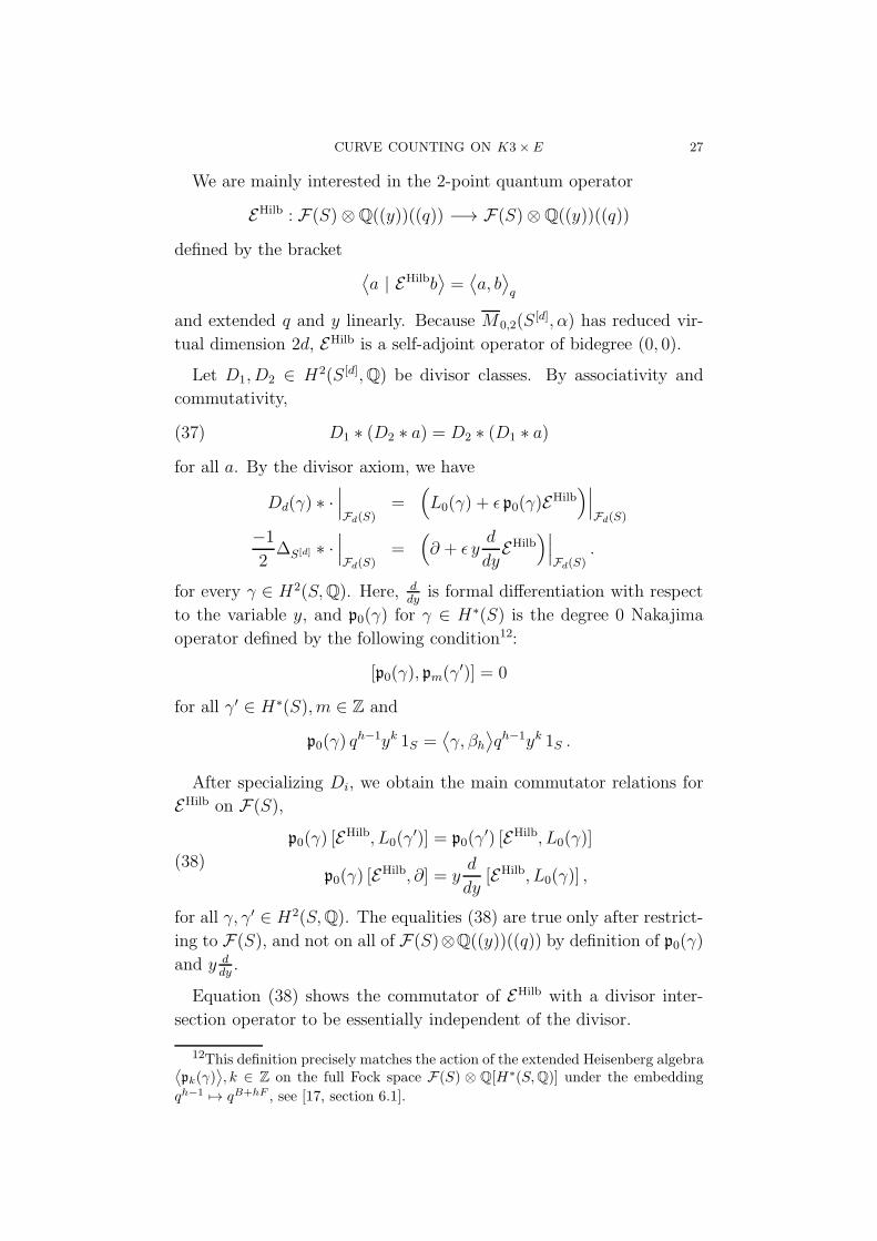
We are mainly interested in the 2-point quantum operator
EHilb : F(S)⊗Q((y))((q)) −→ F(S)⊗Q((y))((q))
defined by the bracket⟨a | EHilbb
⟩=⟨a, b⟩q
and extended q and y linearly. Because M 0,2(S[d], α) has reduced vir-
tual dimension 2d, EHilb is a self-adjoint operator of bidegree (0, 0).
Let D1, D2 ∈ H2(S [d],Q) be divisor classes. By associativity and
commutativity,
(37) D1 ∗ (D2 ∗ a) = D2 ∗ (D1 ∗ a)
for all a. By the divisor axiom, we have
Dd(γ) ∗ ·∣∣∣Fd(S)
=(L0(γ) + ǫ p0(γ)E
Hilb)∣∣∣
Fd(S)
−1
2∆S[d] ∗ ·
∣∣∣Fd(S)
=(∂ + ǫ y
d
dyEHilb
)∣∣∣Fd(S)
.
for every γ ∈ H2(S,Q). Here, ddy
is formal differentiation with respect
to the variable y, and p0(γ) for γ ∈ H∗(S) is the degree 0 Nakajima
operator defined by the following condition12:
[p0(γ), pm(γ′)] = 0
for all γ′ ∈ H∗(S), m ∈ Z and
p0(γ) qh−1yk 1S =
⟨γ, βh
⟩qh−1yk 1S .
After specializing Di, we obtain the main commutator relations for
EHilb on F(S),
(38)
p0(γ) [EHilb, L0(γ
′)] = p0(γ′) [EHilb, L0(γ)]
p0(γ) [EHilb, ∂] = y
d
dy[EHilb, L0(γ)] ,
for all γ, γ′ ∈ H2(S,Q). The equalities (38) are true only after restrict-
ing to F(S), and not on all of F(S)⊗Q((y))((q)) by definition of p0(γ)
and y ddy.
Equation (38) shows the commutator of EHilb with a divisor inter-
section operator to be essentially independent of the divisor.
12This definition precisely matches the action of the extended Heisenberg algebra⟨pk(γ)
⟩, k ∈ Z on the full Fock space F(S) ⊗ Q[H∗(S,Q)] under the embedding
qh−1 7→ qB+hF , see [17, section 6.1].
28 G. OBERDIECK AND R. PANDHARIPANDE
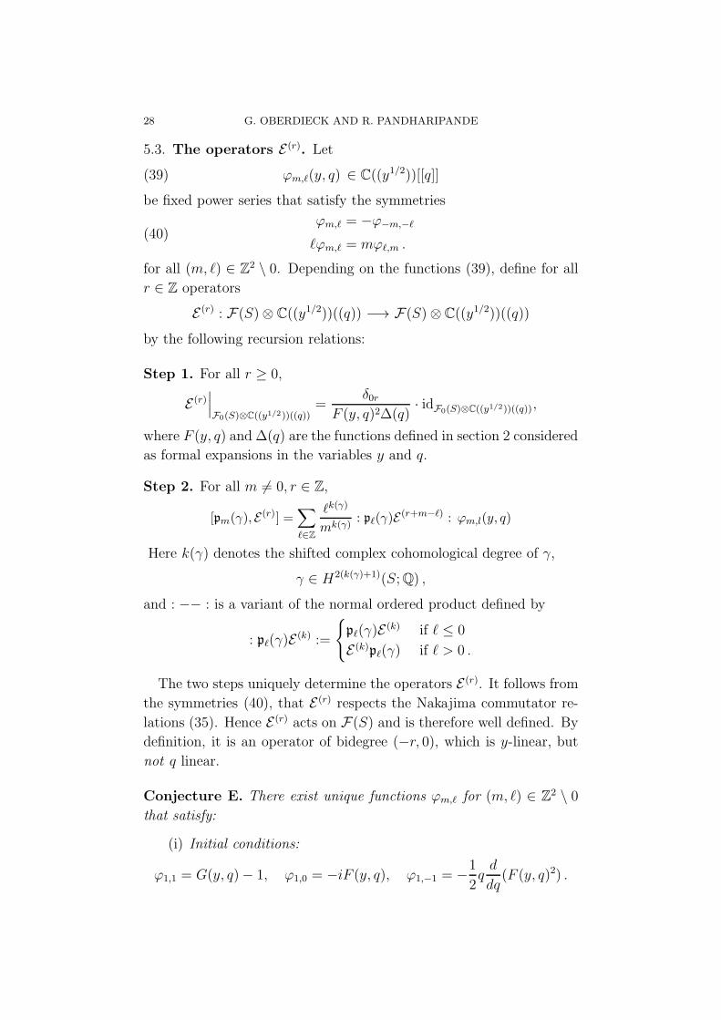
5.3. The operators E (r). Let
(39) ϕm,ℓ(y, q) ∈ C((y1/2))[[q]]
be fixed power series that satisfy the symmetries
(40)ϕm,ℓ = −ϕ−m,−ℓ
ℓϕm,ℓ = mϕℓ,m .
for all (m, ℓ) ∈ Z2 \ 0. Depending on the functions (39), define for all
r ∈ Z operators
E (r) : F(S)⊗ C((y1/2))((q)) −→ F(S)⊗ C((y1/2))((q))
by the following recursion relations:
Step 1. For all r ≥ 0,
E (r)∣∣∣F0(S)⊗C((y1/2))((q))
=δ0r
F (y, q)2∆(q)· idF0(S)⊗C((y1/2))((q)),
where F (y, q) and ∆(q) are the functions defined in section 2 considered
as formal expansions in the variables y and q.
Step 2. For all m 6= 0, r ∈ Z,
[pm(γ), E(r)] =∑
ℓ∈Z
ℓk(γ)
mk(γ): pℓ(γ)E
(r+m−ℓ) : ϕm,l(y, q)
Here k(γ) denotes the shifted complex cohomological degree of γ,
γ ∈ H2(k(γ)+1)(S;Q) ,
and : −− : is a variant of the normal ordered product defined by
: pℓ(γ)E(k) :=
pℓ(γ)E
(k) if ℓ ≤ 0
E (k)pℓ(γ) if ℓ > 0 .
The two steps uniquely determine the operators E (r). It follows from
the symmetries (40), that E (r) respects the Nakajima commutator re-
lations (35). Hence E (r) acts on F(S) and is therefore well defined. By
definition, it is an operator of bidegree (−r, 0), which is y-linear, but
not q linear.
Conjecture E. There exist unique functions ϕm,ℓ for (m, ℓ) ∈ Z2 \ 0
that satisfy:
(i) Initial conditions:
ϕ1,1 = G(y, q)− 1, ϕ1,0 = −iF (y, q), ϕ1,−1 = −1
2qd
dq(F (y, q)2) .
CURVE COUNTING ON K3× E 29
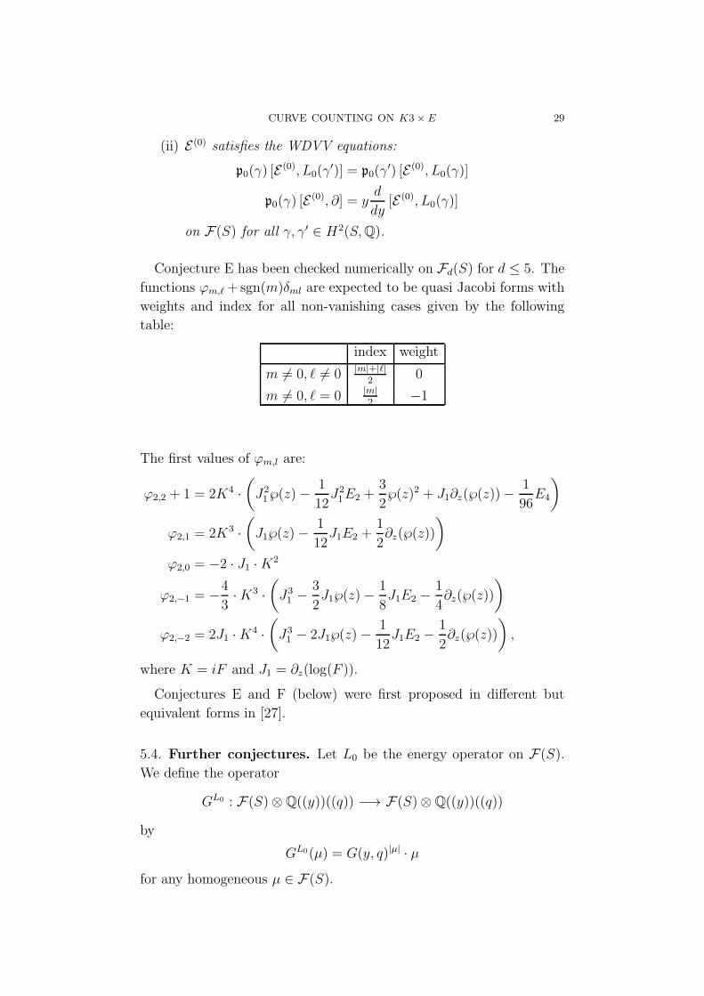
(ii) E (0) satisfies the WDVV equations:
p0(γ) [E(0), L0(γ
′)] = p0(γ′) [E (0), L0(γ)]
p0(γ) [E(0), ∂] = y
d
dy[E (0), L0(γ)]
on F(S) for all γ, γ′ ∈ H2(S,Q).
Conjecture E has been checked numerically on Fd(S) for d ≤ 5. The
functions ϕm,ℓ+ sgn(m)δml are expected to be quasi Jacobi forms with
weights and index for all non-vanishing cases given by the following
table:
index weight
m 6= 0, ℓ 6= 0 |m|+|ℓ|2
0
m 6= 0, ℓ = 0 |m|2
−1
The first values of ϕm,l are:
ϕ2,2 + 1 = 2K4 ·
(J21℘(z)−
1
12J21E2 +
3
2℘(z)2 + J1∂z(℘(z))−
1
96E4
)
ϕ2,1 = 2K3 ·
(J1℘(z)−
1
12J1E2 +
1
2∂z(℘(z))
)
ϕ2,0 = −2 · J1 ·K2
ϕ2,−1 = −4
3·K3 ·
(J31 −
3
2J1℘(z)−
1
8J1E2 −
1
4∂z(℘(z))
)
ϕ2,−2 = 2J1 ·K4 ·
(J31 − 2J1℘(z)−
1
12J1E2 −
1
2∂z(℘(z))
),
where K = iF and J1 = ∂z(log(F )).
Conjectures E and F (below) were first proposed in different but
equivalent forms in [27].
5.4. Further conjectures. Let L0 be the energy operator on F(S).
We define the operator
GL0 : F(S)⊗Q((y))((q)) −→ F(S)⊗Q((y))((q))
by
GL0(µ) = G(y, q)|µ| · µ
for any homogeneous µ ∈ F(S).
30 G. OBERDIECK AND R. PANDHARIPANDE
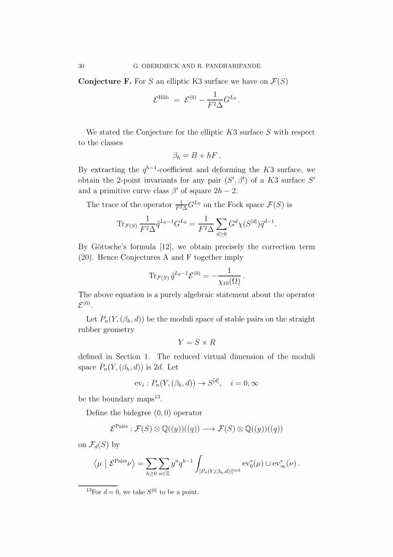
Conjecture F. For S an elliptic K3 surface we have on F(S)
EHilb = E (0) −1
F 2∆GL0 .
We stated the Conjecture for the elliptic K3 surface S with respect
to the classes
βh = B + hF .
By extracting the qh−1-coefficient and deforming the K3 surface, we
obtain the 2-point invariants for any pair (S ′, β ′) of a K3 surface S ′
and a primitive curve class β ′ of square 2h− 2.
The trace of the operator 1F 2∆
GL0 on the Fock space F(S) is
TrF(S)1
F 2∆qL0−1GL0 =
1
F 2∆
∑
d≥0
Gdχ(S [d])qd−1.
By Gottsche’s formula [12], we obtain precisely the correction term
(20). Hence Conjectures A and F together imply
TrF(S) qL0−1E (0) = −
1
χ10(Ω).
The above equation is a purely algebraic statement about the operator
E (0).
Let Pn(Y, (βh, d)) be the moduli space of stable pairs on the straight
rubber geometry
Y = S ×R
defined in Section 1. The reduced virtual dimension of the moduli
space Pn(Y, (βh, d)) is 2d. Let
evi : Pn(Y, (βh, d))→ S [d], i = 0,∞
be the boundary maps13.
Define the bidegree (0, 0) operator
EPairs : F(S)⊗Q((y))((q)) −→ F(S)⊗Q((y))((q))
on Fd(S) by
⟨µ∣∣ EPairsν
⟩=∑
h≥0
∑
n∈Z
ynqh−1
∫
[Pn(Y,(βh,d))]redev∗0(µ) ∪ ev∗∞(ν) .
13For d = 0, we take S[0] to be a point.
CURVE COUNTING ON K3× E 31
Conjecture G. On the elliptic K3 surface S,
EHilb +1
F 2∆GL0 = y−L0EPairs.
We have stated Conjecture G as relating EHilb and EPairs. Combining
Conjectures F and G leads to the direct prediction on F(S):
EPairs = yL0 E (0) .
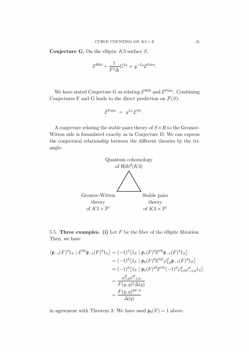
A conjecture relating the stable pairs theory of S×R to the Gromov-
Witten side is formulated exactly as in Conjecture D. We can express
the conjectural relationship between the different theories by the tri-
angle:
Gromov-Witten
theory
of K3× P1
Quantum cohomology
of Hilbd(K3)
Stable pairs
theory
of K3× P1
5.5. Three examples. (i) Let F be the fiber of the elliptic fibration.
Then, we have
⟨p−1(F )
d1S | E(0)p−1(F )
d1S⟩= (−1)d
⟨1S | p1(F )
dE (0)p−1(F )d1S⟩
= (−1)d⟨1S | p0(F )
dE (d)ϕd1,0p−1(F )
d1S⟩
= (−1)d⟨1S | p0(F )
2dE (0)(−1)dϕd1,0ϕ
d−1,01S
⟩
=ϕd1,0ϕ
d−1,0
F (y, q)2∆(q)
=F (y, q)2d−2
∆(q)
in agreement with Theorem 3. We have used p0(F ) = 1 above.
32 G. OBERDIECK AND R. PANDHARIPANDE
(ii) Let W = B+F . Then W 2 = 0 and⟨W,βh
⟩= h− 1. In particular
p0(W ) acts as ∂τ = q ddq. We have
⟨p−1(W )d1S | E
(0)p−1(W )d1S
⟩= (−1)d
⟨1S | p0(W )dE (d)ϕd
1,0p−1(W )d1S⟩
=⟨1S | p0(W )2dE (0)ϕd
1,0ϕd−1,01S
⟩
= ∂2dτ
(ϕd1,0ϕ
d−1,0
F (y, q)2∆(q)
)
= ∂2dτ
(F (y, q)2d−2
∆(q)
).
(iii) Let p ∈ H4(S;Z) be the class of a point. For all d ≥ 1, let
C(F ) = p−1(F )p−1(p)d−11S ∈ H2(S
[d],Z) .
Then, assuming Conjecture F,⟨C(F )
⟩q=⟨C(F ), Dd(F )
⟩q
=1
(d− 1)!
⟨p−1(F )p−1(p)
d−11S | E(0)p−1(F )p−1(e)
d−11S⟩
=1
(d− 1)!
⟨p−1(p)
d−11S | E(0)ϕ1,0ϕ−1,0p−1(e)
d−11S⟩
=(−1)d−1
(d− 1)!
⟨1S | E
(0)ϕ1,0ϕ−1,0(ϕ1,1 + 1)d−1p1(p)
d−1p−1(e)
d−11S⟩
=ϕ1,0ϕ−1,0(ϕ1,1 + 1)d−1
F (y, q)2∆(q)
=G(y, q)d−1
∆(q)
in full agreement with the first part of Theorem 2 in [27].
5.6. The A1 resolution. Let
EPairsB = [q−1]EPairs and EHilbB = [q−1]EHilb
be the restriction of EHilb and EPairs to the case of the class β0 = B.14
The corresponding local case was considered before in [22, 23]. Define
operators E(r)B by
⟨1S | E
(r)B 1S
⟩=
y
(1 + y)2δ0r
[pm(γ), E(r)B ] =
⟨γ, B
⟩ ((−y)−m/2 − (−y)m/2
)E(r+m)B
14We denote with [q−1] the operator that extracts the q−1 coefficient.
CURVE COUNTING ON K3× E 33
for all m 6= 0 and γ ∈ H∗(S), see [23, Section 5.1]. Translating the
results of [22, 23] to the K3 surface leads to the following evaluation.
Theorem 6. We have
EHilbB +
y
(1 + y)2IdF(S) = y−L0EPairsB = E
(0)B .
From numerical experiments [27], we expect the expansions
ϕm,0 =((−y)−m/2 − (−y)m/2
)+O(q) for all m 6= 0
ϕm,ℓ = O(q) for all ℓ 6= 0, m ∈ Z .
Because of
[q−1]GL0
F 2∆=
y
(1 + y)2IdF(S) ,
we find conjectures F and G to be in complete agreement with Theorem
6.
From Theorem 6, we obtain the interesting relation
TrF(S) qL0−1EPairsB =
1
y + 2 + y−1
1
q
∏
m≥1
1
(1 + y−1qm)2(1− qm)20(1 + yqm)2.
By the symmetry of χ10 in the variables q and q, we obtain agreement
with Conjecture A.
6. Motivic theory
Let S be a nonsingular projective K3 surface, and let β ∈ Pic(S)
be a positive class (with respect to any ample polarization). We will
assume β is irreducible (not expressible as a sum of effective classes).
To unify our study with [14], we end the paper with a discussion of
the motivic stable pairs invariants of
X = S × E
in class (β, d). Following the conjectural perspective of [14], we assume
the Betti realization of the motivic invariants of X is both well-defined
and independent of deformations of S for which β remains algebraic
and irreducible.
We define a generating function Z of the Betti realizations of the
motivic stable pairs theory ofX in classes (βh, d) where βh is irreducible
and satisfies
〈βh, βh〉 = 2h− 2 .
34 G. OBERDIECK AND R. PANDHARIPANDE
The series Z depends upon the variables y, q, q just as before and a
new variable u for the virtual Poincare polynomial:
Z(u, y, q, q) =1
u−1 + 2 + u
∑
h≥0
∑
d≥0
H(Pn(S × E, (βh, d))
)ynqh−1qd−1 .
Here we follow the notation of [14, Section 6] for the normalized virtual
Poincare polynomial
H(Pn(S × E, (βh, d))
)∈ Z[u, u−1] .
In the definition of Z, the prefactor 1u−1+2+u
(the reciprocal of the nor-
malized Poincare polynomial of E) quotients by the translation action
of E on Pn(S ×E, (βh, d)).
Because of the u normalization, we have the following symmetry of
Z in the variable u:
(i) Z(u, y, q, q) = Z(u−1, y, q, q) .
Two further properties which constrain Z are:
(ii) the specialization u = −1 must recover the stable pairs invari-
ants (determined by Conjectures A and D),
Z(−1, y, q, q) = −1
χ10,
(iii) the coefficient of q−1 must specialize to the motivic series of [14,
Section 4],
(uy − 1)(u−1 − y−1
)· Coeff q−1
(Z(u, y, q, q)
)=
∞∏
n=1
1
(1− u−1y−1qn)(1− u−1yqn)(1− qn)20(1− uy−1qn)(1− uyqn),
obtained from the Kawai-Yoshioka calculation [17].
To obtain further constraints, we study the virtual Poincare polyno-
mial
H
(P1−h−d(S ×E, (h, d))/E
)∈ Z[u, u−1]
which arises as
(41) Coeff y1−h−dqh−1qd−1
(Z).
CURVE COUNTING ON K3× E 35
For qh−1qd−1, the coefficient (41) corresponds to the the lowest order
term in y. We have an isomorphism of the moduli spaces15,
P1−h−d(S ×E, (h, d))/E ∼= P1−h+d(S, h) .
Hence, we obtain a fourth constraint for Z.
(iv) Coeff y1−h−dqh−1qd−1
(Z)equals the y1−h+dqh−1 coefficient of
1
(uy − 1) (u−1 − y−1)
∞∏
n=1
1
(1 − u−1y−1qn)(1 − u−1yqn)(1 − qn)20(1− uy−1qn)(1− uyqn)
The function − 1χ10
has a basic symmetry in the variables q and q.
As stated, condition (iv) is not symmetric in q and q. However, the
symmetry
Coeff y1−h−dqh−1qd−1
(Z)= Coeff y1−h−dqd−1qh−1
(Z)
can be easily verified from (iv). Unfortunately, further calculations
show that the symmetry in the variables q and q appears not to lift to
the motivic theory.
A basic question is to specify the modular properties of Z. We
hope conditions (i)-(iv) together with the modular properties of Z will
uniquely determine Z. There is every reason to expect the function Z
will be beautiful.
References
[1] A. Beauville, Varietes Kahleriennes dont la premiere classe de Chern est nulle,J. Differential Geom. 18 (1984), 755–782.
[2] K. Behrend, The product formula for Gromov-Witten invariants, J. alg. Geom.8 (1999), 529–541.
[3] J. Bruinier, G. van der Geer, G. Harder, and D. Zagier, The 1-2-3 of modularforms, Springer Verlag: Berlin, 2008.
[4] J. Bryan, The Donaldson-Thomas theory of K3×E via the topological vertex,arXiv:1504.02920.
[5] J. Bryan and C. Leung, The enumerative geometry of K3 surfaces and modularforms, JAMS 13 (2000), 549–568.
[6] J. Bryan and R. Pandharipande, The local Gromov-Witten theory of curves,J. Amer. Math. Soc. 21 (2008), 101–136.
[7] A. Dabholkar, S. Murthy, and D. Zagier, Quantum black holes, wall crossing,and mock modular forms, arXiv:1208.4074.
[8] M. Eichler and D. Zagier, The theory of Jacobi forms, volume 55 of Progress
in Mathematics, Birkhauser Boston Inc., Boston, MA, 1985.[9] C. Faber and R. Pandharipande. Hodge integrals and Gromov-Witten theory,
Invent. Math., 139 (2000), 173–199.
15We follow the notation of [14] for the moduli of stable pairs Pn(S, h) on K3surfaces.
36 G. OBERDIECK AND R. PANDHARIPANDE
[10] A. Gathmann, GROWI: a C++ program for Gromov-Witten invariants,www.mathematik.uni-kl.de/agag/mitglieder/professoren/gathmann/software/growi/ .
[11] A. Gathmann, The number of plane conics that are 5-fold tangent to a givencurve, Compos. Math. 2 (2005), 487–501.
[12] L. Gottsche, The Betti numbers of the Hilbert scheme of points on a smoothprojective surface, Math. Ann. 286 (1990), 193–207.
[13] V. A. Gritsenko and V. V. Nikulin, Siegel automorphic form corrections of
some Lorentzian Kac-Moody Lie algebras, Amer. J. Math. 119 (1997), 181–224.
[14] S. Katz, A. Klemm, and R. Pandharipande, On the motivic stable pairs in-variants of K3 surfaces, arXiv:1407.3181.
[15] S. Katz, A. Klemm, and C. Vafa, M-theory, topological strings, and spinningblack holes, Adv. Theor. Math. Phys. 3 (1999), 1445–1537.
[16] T. Kawai, K3 surfaces, Igusa cusp form, and string theory, hep-th/9710016.[17] T. Kawai and K Yoshioka, String partition functions and infinite products,
Adv. Theor. Math. Phys. 4 (2000), 397–485.[18] M. Lehn, Lectures on Hilbert schemes, in Algebraic structures and moduli
spaces, volume 38 of CRM Proc. Lecture Notes, pages 1–30, Amer. Math.Soc., Providence, RI, 2004.
[19] M. Lehn, Chern classes of tautological sheaves on Hilbert schemes of points onsurfaces, Invent. Math. 136 (1999), 157–207.
[20] D. Maulik, N. Nekrasov, A. Okounkov, and R. Pandharipande, Gromov-Wittentheory and Donaldson-Thomas theory. I, Compos. Math., 142 (2006), 1263–1285.
[21] D. Maulik, Gromov-Witten theory of An-resolutions, Geom. and Top. 13
(2009), 1729–1773.[22] D. Maulik and A. Oblomkov, Donaldson-Thomas theory of An×P 1, Compos.
Math. 145 (2009), no. 5, 12491276.[23] D. Maulik and A. Oblomkov, Quantum cohomology of the Hilbert scheme of
points on An-resolutions, JAMS 22 (2009), 1055–1091.[24] D. Maulik and R. Pandharipande, Gromov-Witten theory and Noether-
Lefschetz theory, in A celebration of algebraic geometry, Clay MathematicsProceedings 18, 469–507, AMS (2010).
[25] D. Maulik, R. Pandharipande, and R. Thomas, Curves on K3 surfaces andmodular forms, J. of Topology 3 (2010), 937–996.
[26] H. Nakajima, Lectures on Hilbert schemes of points on surfaces, AMS: Provi-dence, RI, 1999.
[27] G. Oberdieck, Gromov-Witten invariants of the Hilbert scheme of points of aK3 surface, arXiv:1406.1139.
[28] A. Okounkov and R. Pandharipande, Virasoro constraints for target curves,Invent. Math. 163 (2006), 47–108.
[29] A. Okounkov and R. Pandharipande, Quantum cohomology of the Hilbertscheme of points of the plane, Invent. Math. 179 (2010), 523–557.
[30] A. Okounkov and R. Pandharipande, The local Donaldson-Thomas theory ofcurves, Geom. Topol. 14 (2010), 1503–1567.
[31] R. Pandharipande and A. Pixton, Gromov-Witten/Pairs descendent correspon-dence for toric 3-folds, Geom. and Top. (to appear).
[32] R. Pandharipande and A. Pixton, Gromov-Witten/Pairs correspondence forthe quintic 3-fold, arXiv:1206.5490.
[33] R. Pandharipande and R. P. Thomas, Curve counting via stable pairs in thederived category, Invent. Math. 178 (2009), 407–447.
CURVE COUNTING ON K3× E 37
[34] R. Pandharipande and R. P. Thomas, The Katz-Klemm-Vafa conjecture forK3 surfaces, arXiv:1404.6698.
[35] C. T. C. Wall, On the orthogonal groups of unimodular quadratic forms, Math.Ann. 147 (1962), 328–338.
[36] S.-T. Yau and E. Zaslow, BPS states, string duality, and nodal curves on K3,Nucl. Phys. B457 (1995), 484–512.
ETH Zurich, Department of Mathematics
E-mail address : [email protected]
ETH Zurich, Department of Mathematics
E-mail address : [email protected]