![bloch/paper-revision-final3.pdf · GAMMA FUNCTIONS, MONODROMY AND FROBENIUS CONSTANTS SPENCER BLOCH, MASHA VLASENKO Introduction In an important paper [8], Golyshev and …](https://static.fdocument.org/doc/165x107/5fd5acccbe13c65fa4381622/blochpaper-revision-final3pdf-gamma-functions-monodromy-and-frobenius-constants.jpg)
Curvature of (higher) direct images. - · PDF fileand Lt = LjX t. Theorem ... representative...
57
Curvature of (higher) direct images. Conference in honor of Jean-Pierre Demailly, Grenoble 6/6 2017 Bo Berndtsson Chalmers University of Technology
Transcript of Curvature of (higher) direct images. - · PDF fileand Lt = LjX t. Theorem ... representative...

Curvature of (higher) direct images.
Conference in honor of Jean-Pierre Demailly, Grenoble6/6 2017
Bo BerndtssonChalmers University of Technology
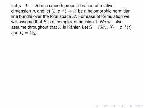
Let p : X → B be a smooth proper fibration of relativedimension n, and let (L,e−φ)→ X be a holomorphic hermitianline bundle over the total space X .
For ease of formulation wewill assume that B is of complex dimension 1. We will alsoassume throughout that X is Kähler. Let Ω = i∂∂φ, Xt = p−1(t)and Lt = L|Xt .
TheoremAssume that Ω ≥ 0. Then there is a holomorphic vector bundle,E, over B with fibers
Et = Hn,0(Xt ,Lt ).
We equip Et with the L2-metric
‖u‖2t = cn
∫Xt
u ∧ ue−φ.
Then (E , ‖ · ‖) has semipositive curvature (in the sense ofNakano).
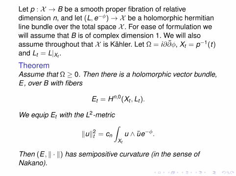
Let p : X → B be a smooth proper fibration of relativedimension n, and let (L,e−φ)→ X be a holomorphic hermitianline bundle over the total space X . For ease of formulation wewill assume that B is of complex dimension 1. We will alsoassume throughout that X is Kähler. Let Ω = i∂∂φ, Xt = p−1(t)and Lt = L|Xt .
TheoremAssume that Ω ≥ 0. Then there is a holomorphic vector bundle,E, over B with fibers
Et = Hn,0(Xt ,Lt ).
We equip Et with the L2-metric
‖u‖2t = cn
∫Xt
u ∧ ue−φ.
Then (E , ‖ · ‖) has semipositive curvature (in the sense ofNakano).
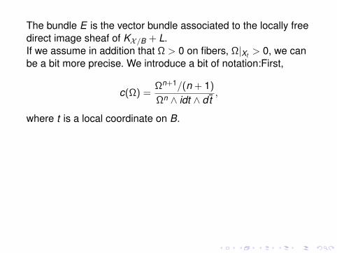
The bundle E is the vector bundle associated to the locally freedirect image sheaf of KX/B + L.
If we assume in addition that Ω > 0 on fibers, Ω|Xt > 0, we canbe a bit more precise. We introduce a bit of notation:First,
c(Ω) =Ωn+1/(n + 1)
Ωn ∧ idt ∧ dt,
where t is a local coordinate on B.
Second, there is a (1,0)- vector field, Vφ, on X , depending onφ, such that dp(Vφ) = ∂
∂t (Vφ is a lift of ∂∂t ), with the property
that Ω(Vφ, W ) = 0 if W is a vertical field ( Vφ is horisontal, seeSiu-Schumacher).
Let κφ = ∂Xt Vφ ∈ Z0,1(T 1,0(Xt )). It is a very specialrepresentative of the Kodaira-Spencer cohomology classκ ∈ H0,1(Xt ,T 1,0).
The bundle E is the vector bundle associated to the locally freedirect image sheaf of KX/B + L.If we assume in addition that Ω > 0 on fibers, Ω|Xt > 0, we canbe a bit more precise. We introduce a bit of notation:
First,
c(Ω) =Ωn+1/(n + 1)
Ωn ∧ idt ∧ dt,
where t is a local coordinate on B.
Second, there is a (1,0)- vector field, Vφ, on X , depending onφ, such that dp(Vφ) = ∂
∂t (Vφ is a lift of ∂∂t ), with the property
that Ω(Vφ, W ) = 0 if W is a vertical field ( Vφ is horisontal, seeSiu-Schumacher).
Let κφ = ∂Xt Vφ ∈ Z0,1(T 1,0(Xt )). It is a very specialrepresentative of the Kodaira-Spencer cohomology classκ ∈ H0,1(Xt ,T 1,0).
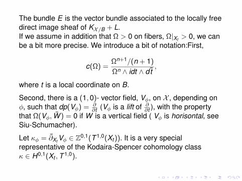
The bundle E is the vector bundle associated to the locally freedirect image sheaf of KX/B + L.If we assume in addition that Ω > 0 on fibers, Ω|Xt > 0, we canbe a bit more precise. We introduce a bit of notation:First,
c(Ω) =Ωn+1/(n + 1)
Ωn ∧ idt ∧ dt,
where t is a local coordinate on B.
Second, there is a (1,0)- vector field, Vφ, on X , depending onφ, such that dp(Vφ) = ∂
∂t (Vφ is a lift of ∂∂t ), with the property
that Ω(Vφ, W ) = 0 if W is a vertical field ( Vφ is horisontal, seeSiu-Schumacher).
Let κφ = ∂Xt Vφ ∈ Z0,1(T 1,0(Xt )). It is a very specialrepresentative of the Kodaira-Spencer cohomology classκ ∈ H0,1(Xt ,T 1,0).
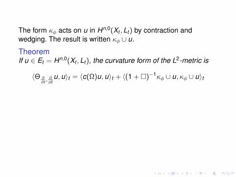
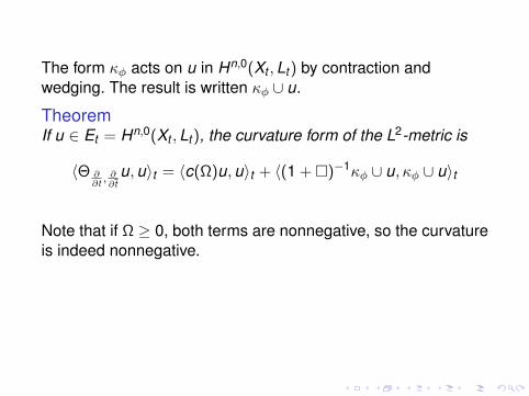
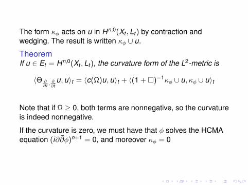
The form κφ acts on u in Hn,0(Xt ,Lt ) by contraction andwedging. The result is written κφ ∪ u.
TheoremIf u ∈ Et = Hn,0(Xt ,Lt ), the curvature form of the L2-metric is
〈Θ ∂∂t ,
∂∂ t
u,u〉t = 〈c(Ω)u,u〉t + 〈(1 + )−1κφ ∪ u, κφ ∪ u〉t
Note that if Ω ≥ 0, both terms are nonnegative, so the curvatureis indeed nonnegative.
If the curvature is zero, we must have that φ solves the HCMAequation (i∂∂φ)n+1 = 0, and moreover κφ = 0
These theorems can be used in several different contexts.
1. To study the variation of complex structure on Xt , eg whenL = mKX/B, m ∈ Z.
2. When the fibration is trivial, X = X × B it can be used tostudy the variation of complex structures on Lt .
3. When the fibration is trivial and the complex structure on Ldoes not change, L = π∗X (L′), L′ a bundle over X , it can be usedto study the variation of metrics on the fixed line bundle L′.Almost equivalently, it can be used to study the variations ofKähler metrics ωt = i∂∂φt in the Mabuchi space of metrics inc[L′].
(When B = t ∈ C; 0 < Re t < 1 and φt = φRe t , c(Ω) is thegeodesic curvature of the curve t → φt in the Mabuchi space. )
These theorems can be used in several different contexts.
1. To study the variation of complex structure on Xt , eg whenL = mKX/B, m ∈ Z.
2. When the fibration is trivial, X = X × B it can be used tostudy the variation of complex structures on Lt .
3. When the fibration is trivial and the complex structure on Ldoes not change, L = π∗X (L′), L′ a bundle over X , it can be usedto study the variation of metrics on the fixed line bundle L′.
Almost equivalently, it can be used to study the variations ofKähler metrics ωt = i∂∂φt in the Mabuchi space of metrics inc[L′].
(When B = t ∈ C; 0 < Re t < 1 and φt = φRe t , c(Ω) is thegeodesic curvature of the curve t → φt in the Mabuchi space. )
These theorems can be used in several different contexts.
1. To study the variation of complex structure on Xt , eg whenL = mKX/B, m ∈ Z.
2. When the fibration is trivial, X = X × B it can be used tostudy the variation of complex structures on Lt .
3. When the fibration is trivial and the complex structure on Ldoes not change, L = π∗X (L′), L′ a bundle over X , it can be usedto study the variation of metrics on the fixed line bundle L′.Almost equivalently, it can be used to study the variations ofKähler metrics ωt = i∂∂φt in the Mabuchi space of metrics inc[L′].
(When B = t ∈ C; 0 < Re t < 1 and φt = φRe t , c(Ω) is thegeodesic curvature of the curve t → φt in the Mabuchi space. )
These theorems can be used in several different contexts.
1. To study the variation of complex structure on Xt , eg whenL = mKX/B, m ∈ Z.
2. When the fibration is trivial, X = X × B it can be used tostudy the variation of complex structures on Lt .
3. When the fibration is trivial and the complex structure on Ldoes not change, L = π∗X (L′), L′ a bundle over X , it can be usedto study the variation of metrics on the fixed line bundle L′.Almost equivalently, it can be used to study the variations ofKähler metrics ωt = i∂∂φt in the Mabuchi space of metrics inc[L′].
(When B = t ∈ C; 0 < Re t < 1 and φt = φRe t , c(Ω) is thegeodesic curvature of the curve t → φt in the Mabuchi space. )
There is also an analog of the second thm for the negativebundle −L. This is about the bundle E∗ with fibersH0,n(Xt ,−Lt ). This bundle has negative curvature.
Example: Take n = 1, Lt = KXt , i e L = KX/B. Assume Lt > 0,so that all fibers are compact Riemann surfaces of genus atleast 2. Then
H0,n(Xt ,−Lt ) = H0,1(Xt ,T 1,0),
which is where KS-classes live. We can take φt to be thepotential of the Kähler-Einstein metric on Xt . ‖u‖2 is theWeil-Peterson norm of u. So we get a formula for the curvatureof the WP-metric.(Wolpert -84)
If we combine the theorem with a theorem of Schumacherwhich says that c(Ω) ≥ 0, we also find that the curvature of theWP-metric is negative (Ahlfors).
Shortly after Wolpert’s work, Siu considered the WP-metric forn = 1, KXt > 0. We are then still looking at the vector bundlewith fibers Et = H0,1(Xt ,T 1,0(Xt )). The WP-metric is theL2-metric on this space for the Kähler-Einstein metric on Xt . Siu(-86) found an explicit formula for the curvature.
We can make this fit the previous discussion by looking at thebundle En,0 with fibers Hn,0(Xt ,−KXt ) = C. This is a trivialbundle with u0 = 1 as trivializing section. Takeκ ∈ H0,1(Xt ,T 1,0(Xt )) and associate to κ,u1 := κ ∪ u0 ∈ Hn−1,1(Xt ,−KXt ). Then ‖κ‖ = ‖u1‖, so we caninterpret Siu’s formula as a curvature formula for En−1,1.
More generally we can look at the bundles Ep,q with fibersHp,q(Xt ,−KXt ), endowed with the L2-metric induced by theKE-metric, for p + q = n. Schumacher (-10) generalized Siu’sformula to all Ep,q, p + q = n.
In joint work with M Paun and X Wang we generalized this asfollows:
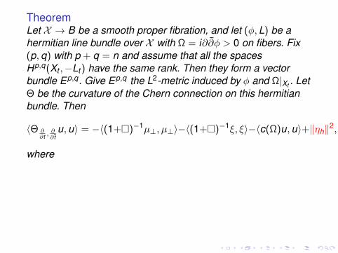
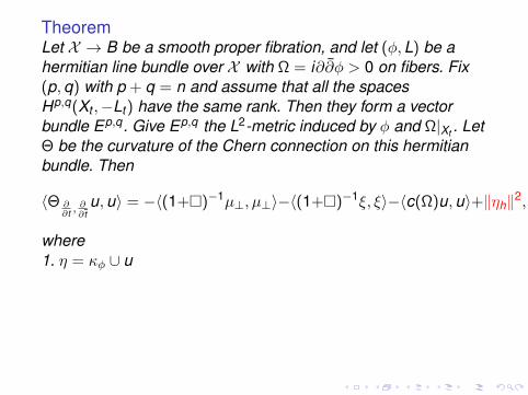
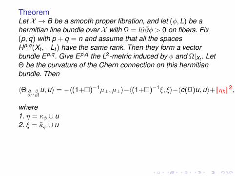
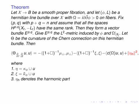
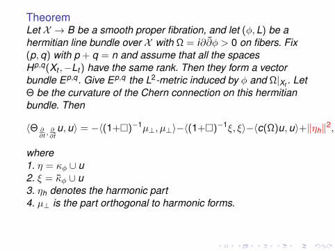
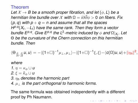
TheoremLet X → B be a smooth proper fibration, and let (φ,L) be ahermitian line bundle over X with Ω = i∂∂φ > 0 on fibers. Fix(p,q) with p + q = n and assume that all the spacesHp,q(Xt ,−Lt ) have the same rank. Then they form a vectorbundle Ep,q. Give Ep,q the L2-metric induced by φ and Ω|Xt . LetΘ be the curvature of the Chern connection on this hermitianbundle. Then
〈Θ ∂∂t ,
∂∂ t
u,u〉 = −〈(1+)−1µ⊥, µ⊥〉−〈(1+)−1ξ, ξ〉−〈c(Ω)u,u〉+‖ηh‖2,
where
1. η = κφ ∪ u2. ξ = κφ ∪ u3. ηh denotes the harmonic part4. µ⊥ is the part orthogonal to harmonic forms.
The same formula was obtained independently with a differentproof by Ph Naumann.
TheoremLet X → B be a smooth proper fibration, and let (φ,L) be ahermitian line bundle over X with Ω = i∂∂φ > 0 on fibers. Fix(p,q) with p + q = n and assume that all the spacesHp,q(Xt ,−Lt ) have the same rank. Then they form a vectorbundle Ep,q. Give Ep,q the L2-metric induced by φ and Ω|Xt . LetΘ be the curvature of the Chern connection on this hermitianbundle. Then
〈Θ ∂∂t ,
∂∂ t
u,u〉 = −〈(1+)−1µ⊥, µ⊥〉−〈(1+)−1ξ, ξ〉−〈c(Ω)u,u〉+‖ηh‖2,
where1. η = κφ ∪ u
2. ξ = κφ ∪ u3. ηh denotes the harmonic part4. µ⊥ is the part orthogonal to harmonic forms.
The same formula was obtained independently with a differentproof by Ph Naumann.
TheoremLet X → B be a smooth proper fibration, and let (φ,L) be ahermitian line bundle over X with Ω = i∂∂φ > 0 on fibers. Fix(p,q) with p + q = n and assume that all the spacesHp,q(Xt ,−Lt ) have the same rank. Then they form a vectorbundle Ep,q. Give Ep,q the L2-metric induced by φ and Ω|Xt . LetΘ be the curvature of the Chern connection on this hermitianbundle. Then
〈Θ ∂∂t ,
∂∂ t
u,u〉 = −〈(1+)−1µ⊥, µ⊥〉−〈(1+)−1ξ, ξ〉−〈c(Ω)u,u〉+‖ηh‖2,
where1. η = κφ ∪ u2. ξ = κφ ∪ u
3. ηh denotes the harmonic part4. µ⊥ is the part orthogonal to harmonic forms.
The same formula was obtained independently with a differentproof by Ph Naumann.
TheoremLet X → B be a smooth proper fibration, and let (φ,L) be ahermitian line bundle over X with Ω = i∂∂φ > 0 on fibers. Fix(p,q) with p + q = n and assume that all the spacesHp,q(Xt ,−Lt ) have the same rank. Then they form a vectorbundle Ep,q. Give Ep,q the L2-metric induced by φ and Ω|Xt . LetΘ be the curvature of the Chern connection on this hermitianbundle. Then
〈Θ ∂∂t ,
∂∂ t
u,u〉 = −〈(1+)−1µ⊥, µ⊥〉−〈(1+)−1ξ, ξ〉−〈c(Ω)u,u〉+‖ηh‖2,
where1. η = κφ ∪ u2. ξ = κφ ∪ u3. ηh denotes the harmonic part
4. µ⊥ is the part orthogonal to harmonic forms.
The same formula was obtained independently with a differentproof by Ph Naumann.
TheoremLet X → B be a smooth proper fibration, and let (φ,L) be ahermitian line bundle over X with Ω = i∂∂φ > 0 on fibers. Fix(p,q) with p + q = n and assume that all the spacesHp,q(Xt ,−Lt ) have the same rank. Then they form a vectorbundle Ep,q. Give Ep,q the L2-metric induced by φ and Ω|Xt . LetΘ be the curvature of the Chern connection on this hermitianbundle. Then
〈Θ ∂∂t ,
∂∂ t
u,u〉 = −〈(1+)−1µ⊥, µ⊥〉−〈(1+)−1ξ, ξ〉−〈c(Ω)u,u〉+‖ηh‖2,
where1. η = κφ ∪ u2. ξ = κφ ∪ u3. ηh denotes the harmonic part4. µ⊥ is the part orthogonal to harmonic forms.
The same formula was obtained independently with a differentproof by Ph Naumann.
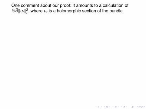
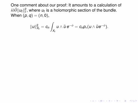
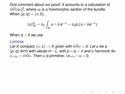
One comment about our proof: It amounts to a calculation ofi∂∂‖ut‖2t , where ut is a holomorphic section of the bundle.
When (p,q) = (n,0),
‖u‖2Xt= cn
∫Xt
u ∧ u e−φ = cnp∗(u ∧ ue−φ).
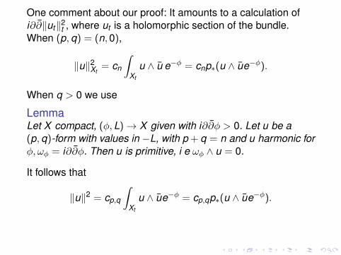
When q > 0 we use
LemmaLet X compact, (φ,L)→ X given with i∂∂φ > 0. Let u be a(p,q)-form with values in −L, with p + q = n and u harmonic forφ, ωφ = i∂∂φ. Then u is primitive, i e ωφ ∧ u = 0.
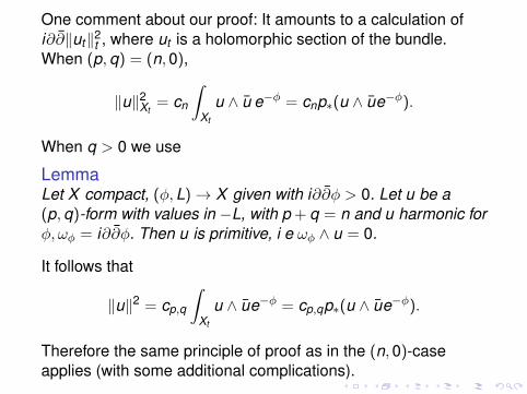
It follows that
‖u‖2 = cp,q
∫Xt
u ∧ ue−φ = cp,qp∗(u ∧ ue−φ).
Therefore the same principle of proof as in the (n,0)-caseapplies (with some additional complications).
One comment about our proof: It amounts to a calculation ofi∂∂‖ut‖2t , where ut is a holomorphic section of the bundle.When (p,q) = (n,0),
‖u‖2Xt= cn
∫Xt
u ∧ u e−φ = cnp∗(u ∧ ue−φ).
When q > 0 we use
LemmaLet X compact, (φ,L)→ X given with i∂∂φ > 0. Let u be a(p,q)-form with values in −L, with p + q = n and u harmonic forφ, ωφ = i∂∂φ. Then u is primitive, i e ωφ ∧ u = 0.
It follows that
‖u‖2 = cp,q
∫Xt
u ∧ ue−φ = cp,qp∗(u ∧ ue−φ).
Therefore the same principle of proof as in the (n,0)-caseapplies (with some additional complications).
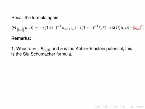
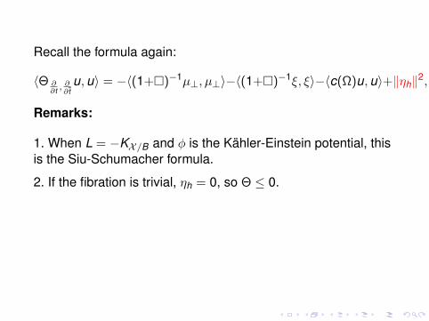
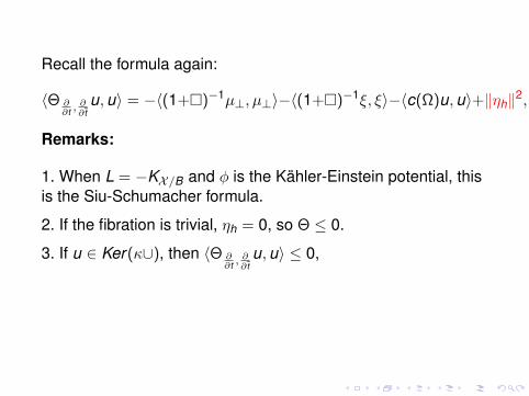
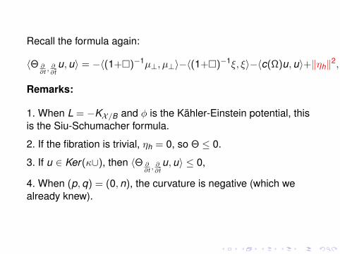
Recall the formula again:
〈Θ ∂∂t ,
∂∂ t
u,u〉 = −〈(1+)−1µ⊥, µ⊥〉−〈(1+)−1ξ, ξ〉−〈c(Ω)u,u〉+‖ηh‖2,
Remarks:
1. When L = −KX/B and φ is the Kähler-Einstein potential, thisis the Siu-Schumacher formula.
2. If the fibration is trivial, ηh = 0, so Θ ≤ 0.
3. If u ∈ Ker(κ∪), then 〈Θ ∂∂t ,
∂∂ t
u,u〉 ≤ 0,
4. When (p,q) = (0,n), the curvature is negative (which wealready knew).
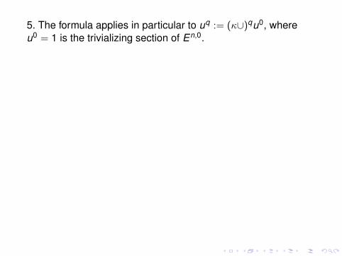
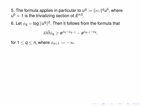
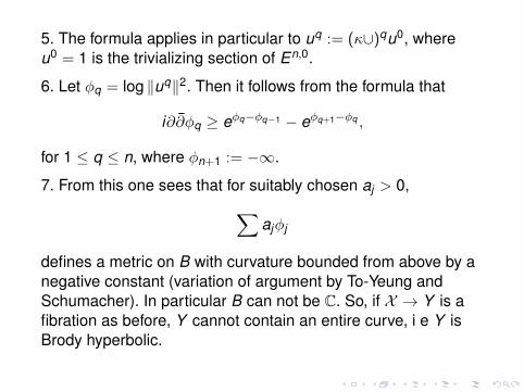
5. The formula applies in particular to uq := (κ∪)qu0, whereu0 = 1 is the trivializing section of En,0.
6. Let φq = log ‖uq‖2. Then it follows from the formula that
i∂∂φq ≥ eφq−φq−1 − eφq+1−φq ,
for 1 ≤ q ≤ n, where φn+1 := −∞.
7. From this one sees that for suitably chosen aj > 0,∑ajφj
defines a metric on B with curvature bounded from above by anegative constant (variation of argument by To-Yeung andSchumacher). In particular B can not be C. So, if X → Y is afibration as before, Y cannot contain an entire curve, i e Y isBrody hyperbolic.
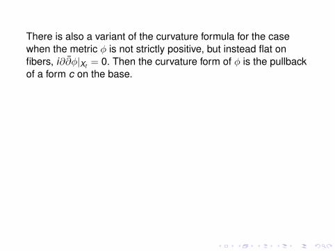
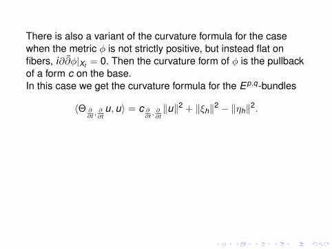
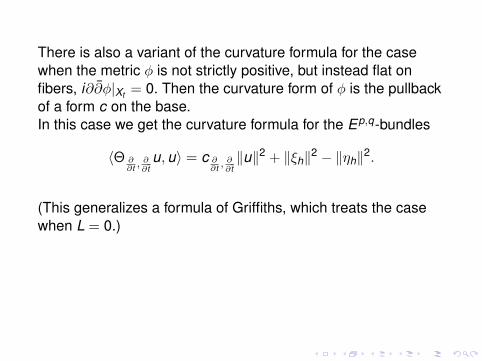
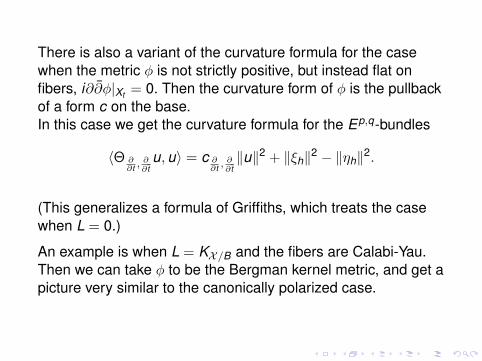
There is also a variant of the curvature formula for the casewhen the metric φ is not strictly positive, but instead flat onfibers, i∂∂φ|Xt = 0. Then the curvature form of φ is the pullbackof a form c on the base.
In this case we get the curvature formula for the Ep,q-bundles
〈Θ ∂∂t ,
∂∂ t
u,u〉 = c ∂∂t ,
∂∂ t‖u‖2 + ‖ξh‖2 − ‖ηh‖2.
(This generalizes a formula of Griffiths, which treats the casewhen L = 0.)
An example is when L = KX/B and the fibers are Calabi-Yau.Then we can take φ to be the Bergman kernel metric, and get apicture very similar to the canonically polarized case.
There is also a variant of the curvature formula for the casewhen the metric φ is not strictly positive, but instead flat onfibers, i∂∂φ|Xt = 0. Then the curvature form of φ is the pullbackof a form c on the base.In this case we get the curvature formula for the Ep,q-bundles
〈Θ ∂∂t ,
∂∂ t
u,u〉 = c ∂∂t ,
∂∂ t‖u‖2 + ‖ξh‖2 − ‖ηh‖2.
(This generalizes a formula of Griffiths, which treats the casewhen L = 0.)
An example is when L = KX/B and the fibers are Calabi-Yau.Then we can take φ to be the Bergman kernel metric, and get apicture very similar to the canonically polarized case.
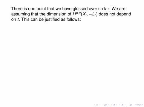
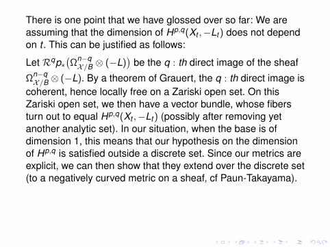
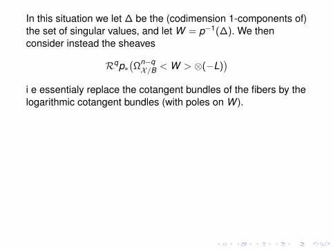
There is one point that we have glossed over so far: We areassuming that the dimension of Hp,q(Xt ,−Lt ) does not dependon t . This can be justified as follows:
Let Rqp∗(Ωn−qX/B ⊗ (−L)
)be the q : th direct image of the sheaf
Ωn−qX/B ⊗ (−L). By a theorem of Grauert, the q : th direct image is
coherent, hence locally free on a Zariski open set. On thisZariski open set, we then have a vector bundle, whose fibersturn out to equal Hp,q(Xt ,−Lt ) (possibly after removing yetanother analytic set). In our situation, when the base is ofdimension 1, this means that our hypothesis on the dimensionof Hp,q is satisfied outside a discrete set. Since our metrics areexplicit, we can then show that they extend over the discrete set(to a negatively curved metric on a sheaf, cf Paun-Takayama).
This suggests yet another extension, to the case when the mapp is not a smooth fibration, but just a surjective map, and mayhave singular fibers over a Zariski closed set.
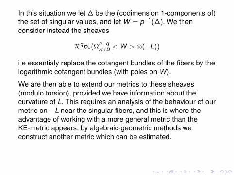
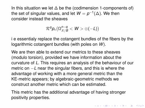
In this situation we let ∆ be the (codimension 1-components of)the set of singular values, and let W = p−1(∆). We thenconsider instead the sheaves
Rqp∗(Ωn−qX/B < W > ⊗(−L)
)i e essentialy replace the cotangent bundles of the fibers by thelogarithmic cotangent bundles (with poles on W ).
We are then able to extend our metrics to these sheaves(modulo torsion), provided we have information about thecurvature of L. This requires an analysis of the behaviour of ourmetric on −L near the singular fibers, and this is where theadvantage of working with a more general metric than theKE-metric appears; by algebraic-geometric methods weconstruct another metric which can be estimated.
This metric has the additional advantage of having strongerpositivity properties.
The net result of all this is a metric version of the followingtheorem of Viehweg-Zhuo.
TheoremLet p : X → Y be a family of canonically polarized manifolds ofmaximal variation. Then there exists a positive q ≤ n such thatthe bundle Symq(ΩY < ∆ >) contains a (non trivial) bigcoherent subsheaf.The subsheaf is essentially the dual of the kernels of theiterated Kodaira-Spencer maps - for which we have a strictnegative bound of the curvature.
The net result of all this is a metric version of the followingtheorem of Viehweg-Zhuo.
TheoremLet p : X → Y be a family of canonically polarized manifolds ofmaximal variation. Then there exists a positive q ≤ n such thatthe bundle Symq(ΩY < ∆ >) contains a (non trivial) bigcoherent subsheaf.
The subsheaf is essentially the dual of the kernels of theiterated Kodaira-Spencer maps - for which we have a strictnegative bound of the curvature.
The net result of all this is a metric version of the followingtheorem of Viehweg-Zhuo.
TheoremLet p : X → Y be a family of canonically polarized manifolds ofmaximal variation. Then there exists a positive q ≤ n such thatthe bundle Symq(ΩY < ∆ >) contains a (non trivial) bigcoherent subsheaf.The subsheaf is essentially the dual of the kernels of theiterated Kodaira-Spencer maps - for which we have a strictnegative bound of the curvature.
Thanks!


![1BDJGJD +PVSOBM PG .BUIFNBUJDT · 150 PETER C. FISHBURN AND JOEL H. SPENCER order on a subset of X. A number of facts about D(P) are sum-marized in [1], which gives other references.](https://static.fdocument.org/doc/165x107/60a42c664d1934206f00f005/1bdjgjd-pvsobm-pg-buifnbujdt-150-peter-c-fishburn-and-joel-h-spencer-order-on.jpg)
![R Carbon - Magritek...Reaction of [Fe(η-C5H5)(η-C6H6)] PF6 with nucleophiles 12 Manuscript prepared by Dr. Almas I. Zayya, Dr. A. Jonathan Singh and Prof. John L. Spencer. School](https://static.fdocument.org/doc/165x107/60bf1c713e8c330af24ff2c3/r-carbon-reaction-of-fe-c5h5-c6h6-pf6-with-nucleophiles-12-manuscript.jpg)