CURRICULUM VITA - Career Account Web Pages - Purdue University
18
A Tutorial Introduction to the Lambda Calculus Raul Rojas * Freie Universit¨at Berlin Version 2.0, 2015 Abstract This paper is a concise and painless introduction to the λ-calculus. This formalism was developed by Alonzo Church as a tool for study- ing the mathematical properties of effectively computable functions. The formalism became popular and has provided a strong theoretical foundation for the family of functional programming languages. This tutorial shows how to perform arithmetical and logical computations using the λ-calculus and how to define recursive functions, even though λ-calculus functions are unnamed and thus cannot refer explicitly to themselves. 1 Definition The λ-calculus can be called the smallest universal programming language in the world . The λ-calculus consists of a single transformation rule (vari- able substitution, also called β -conversion) and a single function definition * Send corrections or suggestions to [email protected] 1
Transcript of CURRICULUM VITA - Career Account Web Pages - Purdue University
A Tutorial Introduction to the LambdaCalculus
Raul Rojas∗
Freie Universitat BerlinVersion 2.0, 2015
Abstract
This paper is a concise and painless introduction to the λ-calculus.This formalism was developed by Alonzo Church as a tool for study-ing the mathematical properties of effectively computable functions.The formalism became popular and has provided a strong theoreticalfoundation for the family of functional programming languages. Thistutorial shows how to perform arithmetical and logical computationsusing the λ-calculus and how to define recursive functions, even thoughλ-calculus functions are unnamed and thus cannot refer explicitly tothemselves.
1 Definition
The λ-calculus can be called the smallest universal programming languagein the world . The λ-calculus consists of a single transformation rule (vari-able substitution, also called β-conversion) and a single function definition
∗Send corrections or suggestions to [email protected]
1

2
scheme. It was introduced in the 1930s by Alonzo Church as a way of for-malizing the concept of effective computability. The λ-calculus is universalin the sense that any computable function can be expressed and evaluatedusing this formalism. It is thus equivalent to Turing machines. However,the λ-calculus emphasizes the use of symbolic transformation rules and doesnot care about the actual machine implementation. It is an approach morerelated to software than to hardware.
The central concept in λ-calculus is that of “expression”. A “name” is anidentifier which, for our purposes, can be any of the letters a, b, c, etc. Anexpression can be just a name or can be a function. Functions use the Greekletter λ to mark the name of the function’s arguments. The “body” of thefunction specifies how the arguments are to be rearranged. The identityfunction, for example, is represented by the string (λx.x). The fragment“λx” tell us that the function’s argument is x, which is returned unchangedas “x” by the function.
Functions can be applied to other functions. The function A, for example,applied to the function B, would be written as AB. In this tutorial, capitalletters are used to represent functions. In fact, anything of interest in λ-calculus is a function. Even numbers or logical values will be representedby functions that can act on one another in order to transform a string ofsymbols into another string. There are no types in λ-calculus: any func-tion can act on any other. The programmer is responsible for keeping thecomputations sensible.
An expression is defined recursively as follows:
< expression > := < name >|< function >|< application >
< function > := λ < name > . < expression >
< application > := < expression >< expression >
An expression can be surrounded by parenthesis for clarity, that is, if E is anexpression, (E) is the same expression. Otherwise, the only keywords used inthe language are λ and the dot. In order to avoid cluttering expressions withparenthesis, we adopt the convention that function application associates

3
from the left, that is, the composite expression
E1E2E3 . . .En
is evaluated applying the successive expressions as follows(. . .((E1E2)E3
). . .En
)As can be seen from the definition of λ-expressions, a well-formed example ofa function is the previously mentioned string, enclosed or not in parentheses:
λx.x ≡ (λx.x)
We use the equivalence symbol “≡” to indicate that when A ≡ B, A is justa synonym for B. As explained above, the name right after the λ is theidentifier of the argument of this function. The expression after the point (inthis case a single x) is called the “body” of the function’s definition.
Functions can be applied to expressions. A simple example of an applicationis
(λx.x)y
This is the identity function applied to the variable y. Parenthesis help toavoid ambiguity. Function applications are evaluated by substituting the“value” of the argument x (in this case the y being processed) in the body ofthe function definition. Fig. 1 shows how the variable y is “absorbed” by thefunction (red line), and also shows where it is used as a replacement for x(green line). The result is a reduction, represented by the right arrow, withthe final result y.
Since we cannot always have pictures, as in Fig. 1, the notation [y/x] is usedto indicate that all occurrences of x are substituted by y in the function’sbody. We write, for example, (λx.x)y → [y/x]x → y. The names of thearguments in function definitions do not carry any meaning by themselves.They are just “place holders”, that is, they are used to indicate how torearrange the arguments of the function when it is evaluated. Therefore allthe strings below represent the same function:
(λz.z) ≡ (λy.y) ≡ (λt.t) ≡ (λu.u)
This kind of purely alphabetical substitution is also called α-reduction.

4
(λx.x)y→ y
(λ∇.∇)y→ y
Figure 1: The same reduction shown twice. The symbol for the function’sargument is just a place holder
1.1 Free and bound variables
If we only had pictures of the plumbing of λ-expressions, we would not haveto care about the names of variables. Since we are using letters as symbols,we have to be careful if we repeat them, as shown in this section.
In λ-calculus all names are local to definitions (like in most programminglanguages). In the function λx.x we say that x is “bound” since its occurrencein the body of the definition is preceded by λx. A name not preceded by aλ is called a “free variable”. In the expression
(λx.x)(λy.yx)
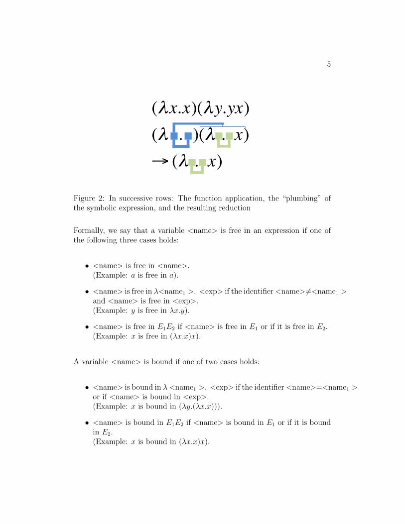
the x in the body of the first expression from the left is bound to the firstλ. The y in the body of the second expression is bound to the second λ,and the following x is free. Bound variables are shown in bold face. Itis very important to notice that this x in the second expression is totallyindependent of the x in the first expression. This can be more easily seenif we draw the “plumbing” of the function application and the consequentreduction, as shown in Fig. 2.
In Fig. 2 we see how the symbolic expression (first row) can be interpretedas a kind of circuit, where the bound argument is moved to a new positioninside the body of the function. The first function (the identity function)“consumes” the second one. The symbol x in the second function has noconnections with the rest of the expression, it is floating free inside the func-tion definition.
5
(λx.x)(λy.yx)(λ . )(λ . x)→ (λ . x)
Figure 2: In successive rows: The function application, the “plumbing” ofthe symbolic expression, and the resulting reduction
Formally, we say that a variable <name> is free in an expression if one ofthe following three cases holds:
• <name> is free in <name>.(Example: a is free in a).
• <name> is free in λ<name1 >. <exp> if the identifier<name>6=<name1 >and <name> is free in <exp>.(Example: y is free in λx.y).
• <name> is free in E1E2 if <name> is free in E1 or if it is free in E2.(Example: x is free in (λx.x)x).
A variable <name> is bound if one of two cases holds:
• <name> is bound in λ <name1 >. <exp> if the identifier<name>=<name1 >or if <name> is bound in <exp>.(Example: x is bound in (λy.(λx.x))).
• <name> is bound in E1E2 if <name> is bound in E1 or if it is boundin E2.(Example: x is bound in (λx.x)x).
6
It should be emphasized that the same identifier can occur free and boundin the same expression. In the expression
(λx.xy)(λy.y)
the first y is free in the parenthesized subexpression to the left, but it isbound in the subexpression to the right. Therefore, it occurs free as well asbound in the whole expression (the bound variables are shown in bold face).
1.2 Substitutions
The more confusing part of standard λ-calculus, when first approaching it,isthe fact that we do not give names to functions. Any time we want to applya function, we just write the complete function’s definition and then proceedto evaluate it. To simplify the notation, however, we will use capital letters,digits and other symbols (san serif) as synonyms for some functions. Theidentity function, for example, can be denoted by the letter I, using it asshorthand for (λx.x).
The identity function applied to itself is the application
II ≡ (λx.x)(λx.x).
In this expression, the first x in the body of the first function in parenthesisis independent of the x in the body of the second function (remember thatthe “plumbing” is local). Just to emphasize the difference we can in factrewrite the above expression as
II ≡ (λx.x)(λz.z).
The identity function applied to itself
II ≡ (λx.x)(λz.z)
yields therefore[(λz.z)/x]x→ λz.z ≡ I,
that is, the identity function again.

7
(λx.(λy.xy))y
(λx.(λy.xy))yy bound in the subexpression
danger: a free y should not be mixed with bound y’s
Figure 3: A free variable should not be substituted in a subexpression whereit is bound, otherwise a new “plumbing”, different to the original, would begenerated
When performing substitutions, we should be careful to avoid mixing up freeoccurrences of an identifier with bound ones. In the expression(
λx.(λy.xy))y
the function on the left contains a bound y, whereas the y on the right isfree. An incorrect substitution would mix the two identifiers in the erroneousresult
(λy.yy).
Simply by renaming the bound y to t we obtain(λx.(λt.xt)
)y → (λt.yt)
which is a completely different result but nevertheless the correct one.
Therefore, if the function λx. < exp > is applied to E, we substitute all freeoccurrences of x in < exp > with E. If the substitution would bring a freevariable of E in an expression where this variable occurs bound, we rename

8
the bound variable before performing the substitution. For example, in theexpression
(λx.(λy.(x(λx.xy)))) y
we associate the first x with y. In the body
(λy.(x(λx.xy)))
only the first x is free and can be substituted. Before substituting though,we have to rename the variable y to avoid mixing its bound with its freeoccurrence:
[y/x] (λt.(x(λx.xt)))→ (λt(y(λx.xt)))
In normal order reduction we try to reduce always the left most expression ofa series of applications. We continue until no further reductions are possible.
2 Arithmetic
A programming language should be capable of specifying arithmetical calcu-lations. Numbers can be represented in the λ-calculus starting from zero andwriting “successor of zero”, that is “suc(zero)”, to represent 1, “suc(suc(zero))”to represent 2, and so on. Since in λ-calculus we can only define new func-tions, numbers will be defined as functions using the following approach: zerocan be defined as
λs.(λz.z)
This is a function of two arguments s and z. We will abbreviate such expres-sions with more than one argument as
λsz.z
It is understood here that s is the first argument to be substituted during theevaluation and z the second. Using this notation, the first natural numberscan be defined as
0 ≡ λsz.z
1 ≡ λsz.s(z)
2 ≡ λsz.s(s(z))
3 ≡ λsz.s(s(s(z)))

9
and so on.
The big advantage of defining numbers in this way is that we can now applya function f to an argument a any number of times. For example, if we wantto apply f to a three times we apply the function 3 to the arguments f anda yielding:
3fa→ (λsz.s(s(sz)))fa→ f(f(fa)).
This way of defining numbers provides us with a language construct similarto an instruction such as “FOR i=1 to 3” in other languages. The numberzero applied to the arguments f and a yields 0fa ≡ (λsz.z)fa→ a. That is,applying the function f to the argument a zero times leaves the argument aunchanged.
Our first interesting function, after having defined the natural numbers, isthe successor function. This can be defined as
S ≡ λnab.a(nab).
The definition looks awkward but it works. For example, the successor func-tion applied to our representation for zero is the expression:
S0 ≡ (λnab.a(nab))0
In the body of the first expression we substitute the occurrence of n with 0and this produces the reduced expression:
λab.a(0ab)→ λab.a(b) ≡ 1
That is, the result is the representation of the number 1 (remember thatbound variable names are “dummies” and can be changed).
Successor applied to 1 yields:
S1 ≡ (λnab.a(nab))1→ λab.a(1ab)→ λab.a(ab) ≡ 2
Notice that the only purpose of applying the number 1 ≡ (λsz.sz) to the ar-guments a and b is to “rename” the variables used internally in the definitionof our number.

10
2.1 Addition
Addition can be obtained immediately by noting that the body sz of ourdefinition of the number 1, for example, can be interpreted as the applicationof the function s on z. If we want to add say 2 and 3, we just apply thesuccessor function two times to 3.
Let us try the following in order to compute 2+3:
2S3 ≡ (λsz.s(sz)))S3→ S(S3)→ S4→ 5
In general m plus n can be computed by the expression mSn.
three applica+ons of s
a
a a a
(λsz.s(s(sz)))a
a applied three +mes
Figure 4: The number 3 applied to an argument a produces a new function
11
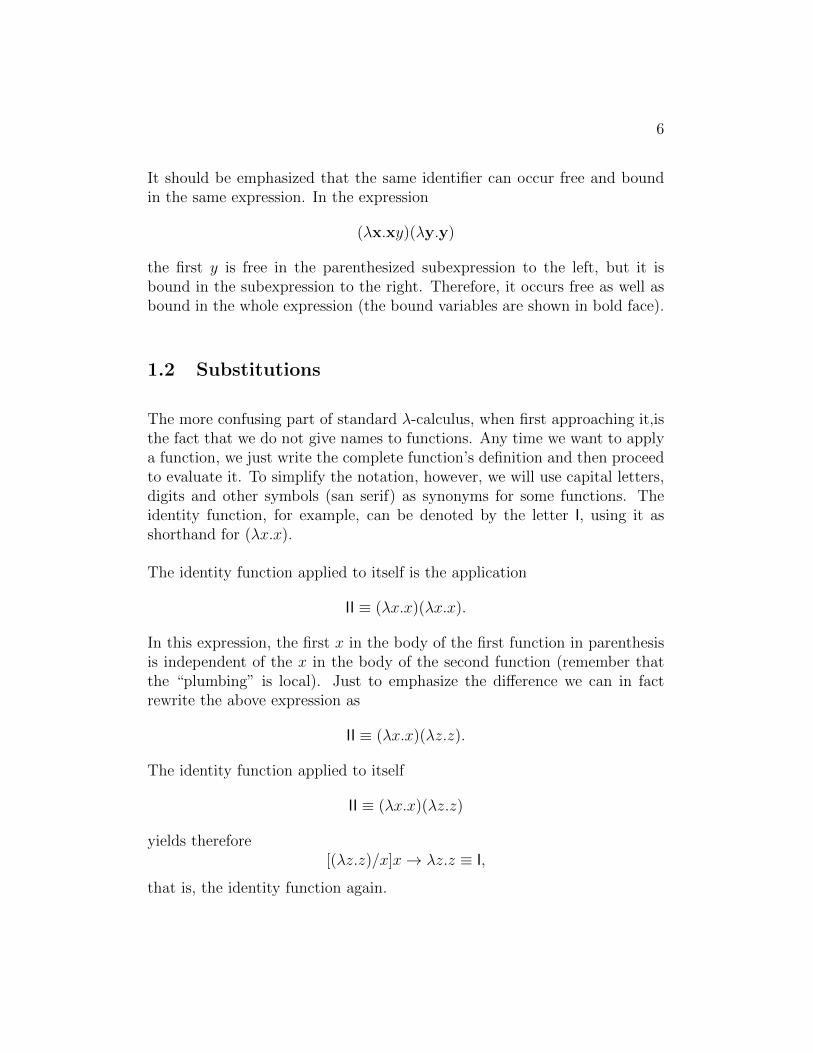
2.2 Multiplication
The multiplication of two numberx x and y can be computed using the fol-lowing function:
(λxya.x(ya))
The product of 3 by 3 is then
(λxya.x(ya))33
which reduces to(λa.3(3a))
a a a
a a a
a a a b
a applied 3 by 3 +mes to b
3(3a)b = a(a(a(a(a(a(a(a(ab))))))))
Figure 5: The plumbing of the function 3 applied to 3a, and the result to b
In order to understand why this function really computes the product of 3by 3, let us look at some diagrams. The first application (3a) is computedin Fig. 4 . Notice that the application of 3 to a has the effect of producing anew function which applies a three times to the function’s argument.
12
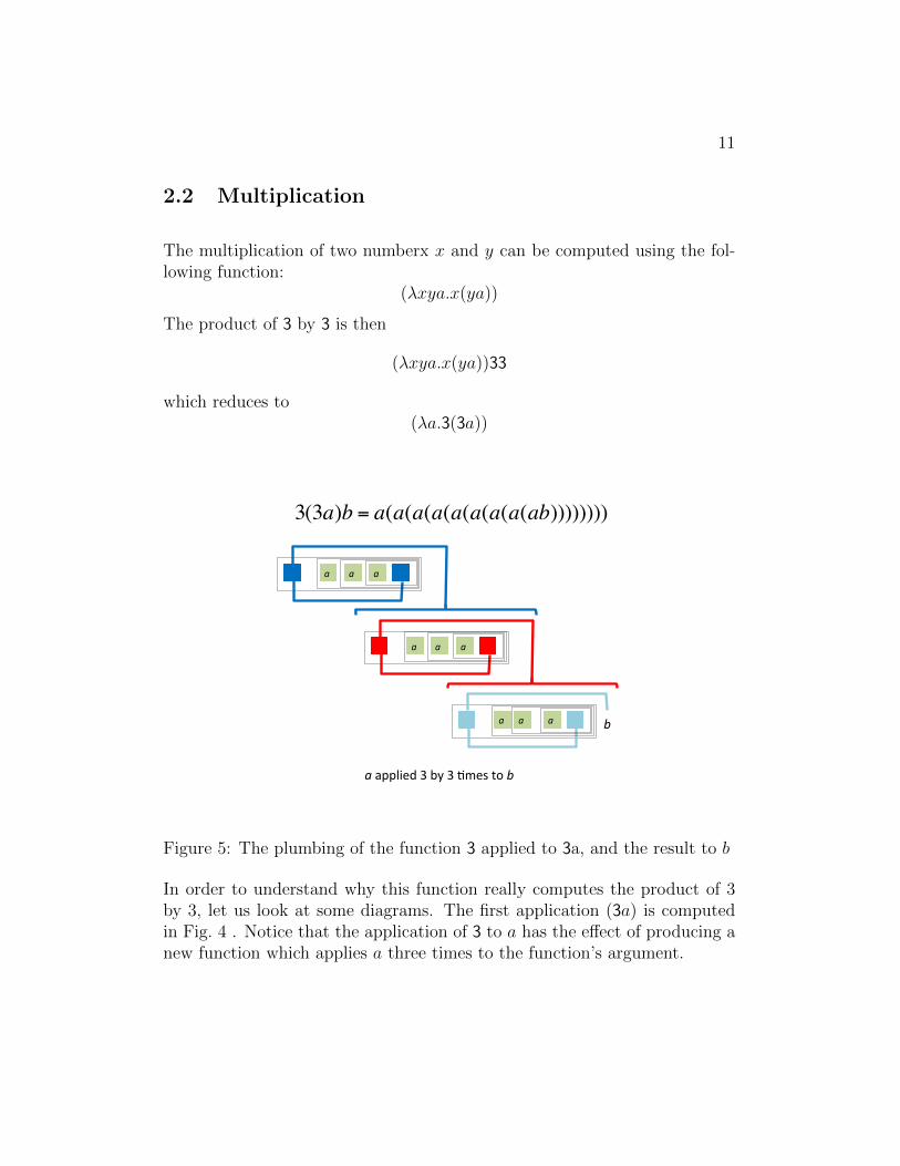
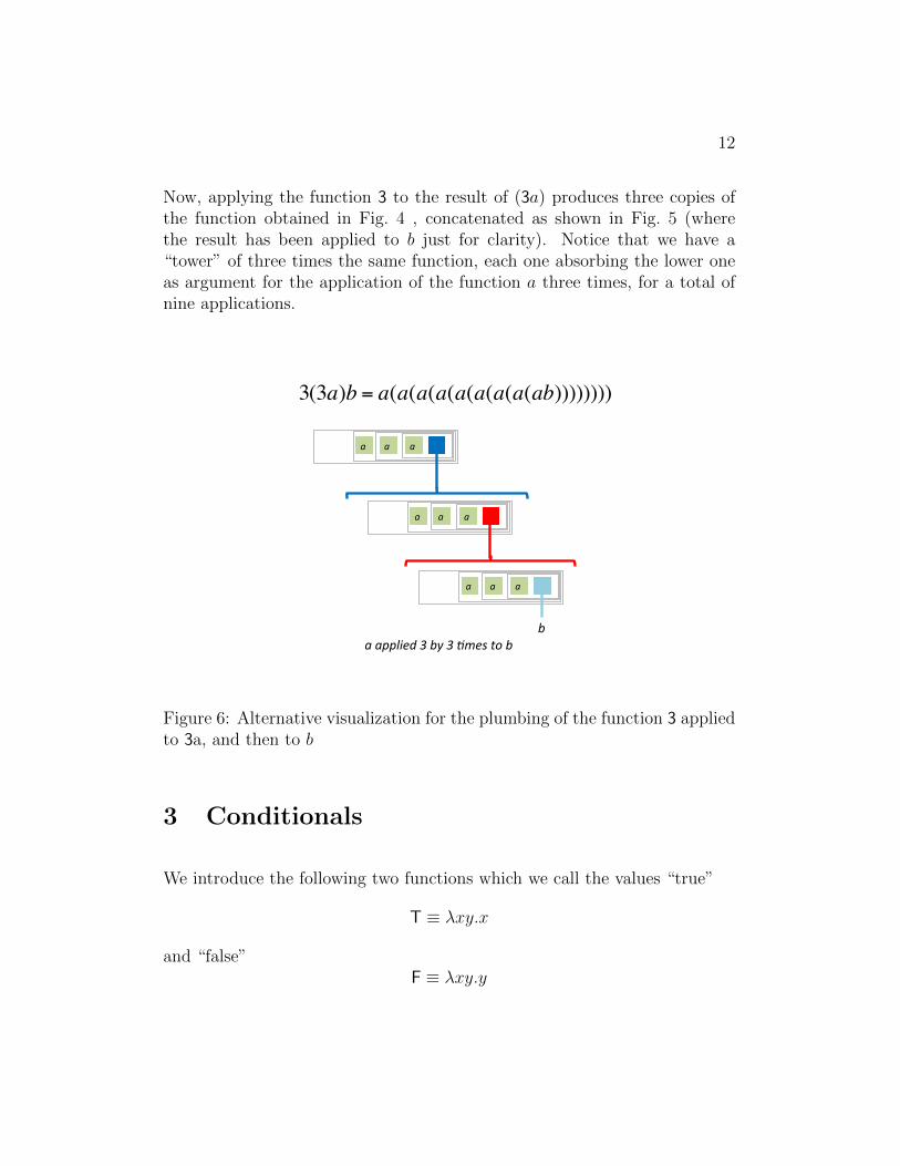
Now, applying the function 3 to the result of (3a) produces three copies ofthe function obtained in Fig. 4 , concatenated as shown in Fig. 5 (wherethe result has been applied to b just for clarity). Notice that we have a“tower” of three times the same function, each one absorbing the lower oneas argument for the application of the function a three times, for a total ofnine applications.
a a a
a a a
a a a
b a applied 3 by 3 +mes to b
3(3a)b = a(a(a(a(a(a(a(a(ab))))))))
Figure 6: Alternative visualization for the plumbing of the function 3 appliedto 3a, and then to b
3 Conditionals
We introduce the following two functions which we call the values “true”
T ≡ λxy.x
and “false”F ≡ λxy.y
13
The first function takes two arguments and returns the first one. The secondfunction returns the second of two arguments.
3.1 Logical operations
It is now possible to define logical operations using this representation of thetruth values.
The AND function of two arguments can be defined as
∧ ≡ λxy.xyF
This definition works because given that x is true, the truth value of theAND operation depends on the truth value of y. If x is false (and selectsthus the second argument in xyF) the complete AND is false, regardless ofthe value of y.
The OR function of two arguments can be defined as
∨ ≡ λxy.xTy
Here, if x is true, the OR is true. If x is false, it picks the second argumenty and the value of the OR function depends now on the value of y.
Negation of one argument can be defined as
¬ ≡ λx.xFT
For example, the negation function applied to “true” is
¬T ≡ (λx.xFT)T
which reduces toTFT ≡ (λcd.c)FT→ F
that is, the truth value “false”.
Armed with this three logic functions we can encode any other logic functionand reproduce any given circuit without feedback (we look at feedback whenwe deal with recursion).
14
3.2 A conditional test
It is very convenient in a programming language to have a function which istrue if a number is zero and false otherwise. The following function Z fulfillsthis role:
Z ≡ λx.xF¬FTo understand how this function works, remember that
0fa ≡ (λsz.z)fa = a
that is, the function f applied zero times to the argument a yields a. On theother hand, F applied to any argument yields the identity function
Fa ≡ (λxy.y)a→ λy.y ≡ I
We can now test if the function Z works correctly. The function applied tozero yields
Z0 ≡ (λx.xF¬F)0→ 0F¬F→ ¬F→ T
because F applied 0 times to ¬ yields ¬. The function Z applied to any othernumber N yields
ZN ≡ (λx.xF¬F)N→ NF¬FThe function F is then applied N times to ¬. But F applied to anything isthe identity (as shown before), so that the above expression reduces, for anynumber N greater than zero, to
IF→ F
3.3 The predecessor function
We can now define the predecessor function combining some of the functionsintroduced above. When looking for the predecessor of n, the general strategywill be to create a pair (n, n − 1) and then pick the second element of thepair as the result.
A pair (a, b) can be represented in λ-calculus using the function
(λz.zab)
15
We can extract the first element of the pair from the expression applying thisfunction to T
(λz.zab)T→ Tab→ a,
and the second applying the function to F
(λz.zab)F→ Fab→ b.
The following function generates from the pair (n, n− 1) (which is the argu-ment p in the function) the pair (n+ 1, n):
Φ ≡ (λpz.z(S(pT))(pT))
The subexpression pT extracts the firs element from the pair p. A new pairis formed using this element, which is incremented for the first position ofthe new pair and just copied for the second position of the new pair.
The predecessor of a number n is obtained by applying n times the functionΦ to the pair (λ.z00) and then selecting the second member of the new pair:
P ≡ (λn.(nΦ(λz.z00))F)
Notice that using this approach the predecessor of zero is zero. This propertyis useful for the definition of other functions.
3.4 Equality and inequalities
With the predecessor function as the building block, we can now define afunction which tests if a number x is greater than or equal to a number y:
G ≡ (λxy.Z(xPy))
If the predecessor function applied x times to y yields zero, then it is truethat x ≥ y.
If x ≥ y and y ≥ x, then x = y. This leads to the following definition of thefunction E which tests if two numbers are equal:
E ≡ (λxy. ∧ (Z(xPy))(Z(yPx)))
In a similar manner we can define functions to test whether x > y, x < y orx 6= y.

16
4 Recursion
Recursive functions can be defined in the λ-calculus using a function whichcalls a function y and then regenerates itself. This can be better understoodby considering the following function Y:
Y ≡ (λy.(λx.y(xx))(λx.y(xx)))
This function applied to a function R yields:
YR ≡ (λx.R(xx))(λx.R(xx))
which further reduced yields
R((λx.R(xx))(λx.R(xx))
but this means that YR→ R(YR), that is, the function R is evaluated usingthe recursive call YR as the first argument.
An infinite loop, for example, can be programmed as YI, since this reducesto I(YI), then to YI and so ad infinitum.
A more useful function is one which adds the first n natural numbers. Wecan use a recursive definition, since
∑ni=0 i = n +
∑n−1i=0 i. Let us use the
following definition for R:
R ≡ (λrn.Zn0(nS(r(Pn))))
This definition tells us that the number n is tested: if it is zero the resultof the sum is zero. In n is not zero, then the successor function is appliedn times to the recursive call (the argument r) of the function applied to thepredecessor of n.
How do we know that r in the expression above is the recursive call to R,since functions in λ-calculus do not have names? We do not know and that isprecisely why we have to use the recursion operator Y. Assume for examplethat we want to add the numbers from 0 to 3. The necessary operations areperformed by the call:
YR3→ R(YR)3→ Z30(3S(YR(P3)))
17
Since 3 is not equal to zero, the evaluation is equivalent to
3S(YR2)
that is, the sum of the numbers from 0 to 3 is equal to 3 plus the sum of thenumbers from 0 to 2. Successive recursive evaluations of YR will lead to thecorrect final result.
Notice that in the function defined above the recursion will be stopped whenthe argument becomes 0. The final result will be
3S(2S(1S0))
that is, the number 6.
Caveat: For the sake of this tutorial I simplified some expressions withoutfollowing the normal reduction order, from left to right. For example, inthe reduction S(S3) → S4 → 5, actually the first successor function will beevaluated before S3. The resulting reductions are rather messy, if done withpaper and pencil, but are easy to perform with a computer. The reader cantry to perform some of those reductions keeping to the left to right reductionorder.
5 Projects for the reader
1. Define the functions “less than” and “greater than” of two numericalarguments.
2. Define the positive and negative integers using pairs of natural numbers.
3. Define addition and subtraction of integers.
4. Define the division of positive integers recursively.
5. Define the function n! = n · (n− 1) · · · 1 recursively.
6. Define the rational numbers as pairs of integers.

18
7. Define functions for the addition, subtraction, multiplication and divi-sion of rationals.
8. Define a data structure to represent a list of numbers.
9. Define a function which extracts the first element from a list.
10. Define a recursive function which counts the number of elements in alist.
11. Can you simulate a Turing machine using λ-calculus?
References
[1] P.M. Kogge, The Architecture of Symbolic Computers , McGraw-Hill, Newyork 1991, chapter 4.
[2] G. Michaelson, An Introduction to Functional Programming through λ-calculus , Addison-Wesley, Wokingham, 1988.
[3] G. Revesz, Lambda-Calculus Combinators and Functional Programming ,Cambridge University Press, Cambridge, 1988, chapters 1-3.