CPSC 540: Machine LearningMetropolis-Hastings

Mark Schmidt

University of British Columbia

Winter 2020

Last Time: Approximate Inference

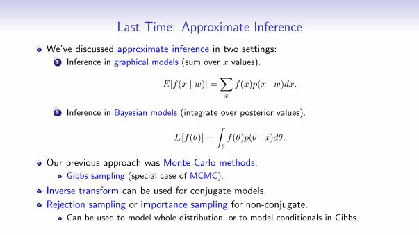
We’ve discussed approximate inference in two settings:1 Inference in graphical models (sum over x values).

E[f(x | w)] =∑x

f(x)p(x | w)dx.

2 Inference in Bayesian models (integrate over posterior values).

E[f(θ)] =

∫θ

f(θ)p(θ | x)dθ.

Our previous approach was Monte Carlo methods.

Gibbs sampling (special case of MCMC).

Inverse transform can be used for conjugate models.

Rejection sampling or importance sampling for non-conjugate.

Can be used to model whole distribution, or to model conditionals in Gibbs.

Limitations of Simple Monte Carlo Methods

The basic ingredients of our previous sampling methods:

Sampling in low dimensions: Inverse CDF, rejection sampling, importance sampling.Sampling in higher dimensions: ancestral sampling, Gibbs sampling.

These work well in low dimensions or for posteriors with analytic properties.

But we want to solve high-dimensional integration problems in other settings:

Deep belief networks and Boltzmann machines.Bayesian graphical models and Bayesian neural networks.Hierarchical Bayesian models.

Our previous methods tend not to work in complex situations:

Inverse CDF may not be available.Conditionals needed for ancestral/Gibbs sampling may be hard to compute.Rejection sampling tends to reject almost all samples.Importance sampling tends to give almost zero weight to all samples.

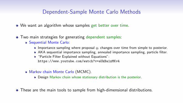
Dependent-Sample Monte Carlo Methods

We want an algorithm whose samples get better over time.

Two main strategies for generating dependent samples:Sequential Monte Carlo:

Importance sampling where proposal qt changes over time from simple to posterior.AKA sequential importance sampling, annealed importance sampling, particle filter.“Particle Filter Explained without Equations”:https://www.youtube.com/watch?v=aUkBa1zMKv4

Markov chain Monte Carlo (MCMC).

Design Markov chain whose stationary distribution is the posterior.

These are the main tools to sample from high-dimensional distributions.

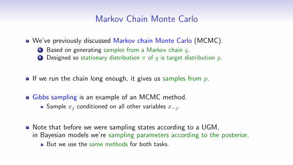
Markov Chain Monte Carlo

We’ve previously discussed Markov chain Monte Carlo (MCMC).1 Based on generating samples from a Markov chain q.2 Designed so stationary distribution π of q is target distribution p.

If we run the chain long enough, it gives us samples from p.

Gibbs sampling is an example of an MCMC method.

Sample xj conditioned on all other variables x−j .

Note that before we were sampling states according to a UGM,in Bayesian models we’re sampling parameters according to the posterior.

But we use the same methods for both tasks.

Limitations of Gibbs Sampling

Gibbs sampling is nice because it has no parameters:

You just need to decide on the blocks and figure out the conditionals.

But it isn’t always ideal:

Samples can be very correlated: slow progress.Conditionals may not have a nice form:

If Markov blanket is not conjugate, need rejection sampling (or numerical CDF).

Generalization that can address these is Metropolis-Hastings:

Oldest algorithm among the “10 Best of the 20th Century”.

Warm-Up to Metropolis-Hastings: “Stupid MCMC”

Consider finding the expected value of a fair di:

For a 6-sided di, the expected value is 3.5.

Consider the following “stupid MCMC” algorithm:

Start with some initial value, like “4”.

At each step, roll the di and generate a random number u:

If u < 0.5, “accept” the roll and take the roll as the next sample.

Othewise, “reject” the roll and take the old value (“4”) as the next sample.

Warm-Up to Metropolis-Hastings: “Stupid MCMC”

Example:

Start with “4”, so record “4”.Roll a “6” and generate 0.234, so record “6”.Roll a “3” and generate 0.612, so record “6”.Roll a “2” and generate 0.523, so record “6”.Roll a “3” and generate 0.125, so record “3”.

So our samples are 4,6,6,6,3,. . .

If you run this long enough, you will spend 1/6 of the time on each number.So the dependent samples from this Markov chain could be used within Monte Carlo.

It is “stupid” since you should just accept every sample (they are IID samples).

It works but it is twice as slow.

A Simple Example of Metropolis-HastingsConsider a loaded di that rolls a 6 half the time (all others equally likely).

So p(x = 6) = 1/2 and p(x = 1) = p(x = 2) = · · · = p(x = 5) = 1/10.

Consider the following “less stupid” MCMC algorithm:At each step, we start with an old state x.Generate a random number x uniformly between 1 and 6 (roll a fair di),and generate a random number u in the interval [0, 1].“Accept” this roll if

u <p(x̂)

p(x).

So if we roll x̂ = 6, we accept it: u < 1 (‘’always move to higher probability”).If x = 2 and roll x̂ = 1, accept it: u < 1 (“always move to same probability”).If x = 6 and roll x̂ = 1, we accept it with probability 1/5.

We prefer high probability states, but sometimes move to low probability states.

This has right probabilities as the stationary distribution (not yet obvious).And accepts most samples.

Metropolis Algorithm

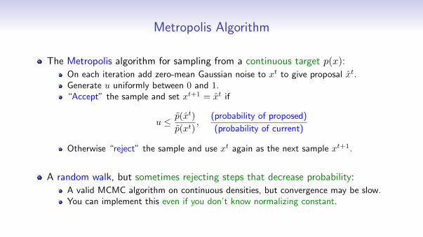
The Metropolis algorithm for sampling from a continuous target p(x):

On each iteration add zero-mean Gaussian noise to xt to give proposal x̂t.Generate u uniformly between 0 and 1.“Accept” the sample and set xt+1 = x̂t if

u ≤ p̃(x̂t)

p̃(xt),

(probability of proposed)

(probability of current)

Otherwise “reject” the sample and use xt again as the next sample xt+1.

A random walk, but sometimes rejecting steps that decrease probability:

A valid MCMC algorithm on continuous densities, but convergence may be slow.You can implement this even if you don’t know normalizing constant.

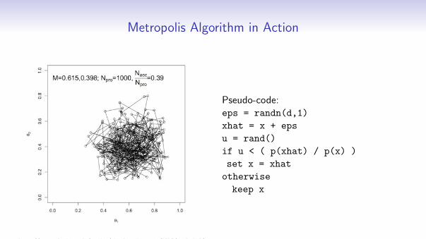
Metropolis Algorithm in Action

http://www.columbia.edu/~cjd11/charles_dimaggio/DIRE/styled-4/

styled-11/code-5

Pseudo-code:eps = randn(d,1)

xhat = x + eps

u = rand()

if u < ( p(xhat) / p(x) )

set x = xhat

otherwise

keep x

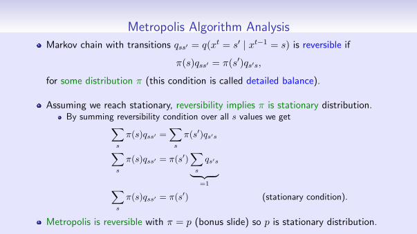
Metropolis Algorithm Analysis

Markov chain with transitions qss′ = q(xt = s′ | xt−1 = s) is reversible if

π(s)qss′ = π(s′)qs′s,

for some distribution π (this condition is called detailed balance).

Assuming we reach stationary, reversibility implies π is stationary distribution.By summing reversibility condition over all s values we get∑

s

π(s)qss′ =∑s

π(s′)qs′s∑s

π(s)qss′ = π(s′)∑s

qs′s︸ ︷︷ ︸=1∑

s

π(s)qss′ = π(s′) (stationary condition).

Metropolis is reversible with π = p (bonus slide) so p is stationary distribution.

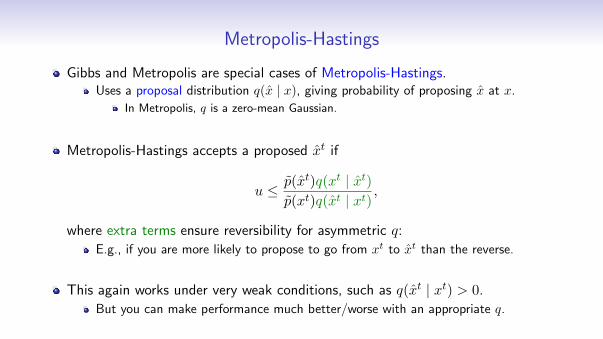
Metropolis-Hastings

Gibbs and Metropolis are special cases of Metropolis-Hastings.Uses a proposal distribution q(x̂ | x), giving probability of proposing x̂ at x.

In Metropolis, q is a zero-mean Gaussian.

Metropolis-Hastings accepts a proposed x̂t if

u ≤ p̃(x̂t)q(xt | x̂t)p̃(xt)q(x̂t | xt)

,

where extra terms ensure reversibility for asymmetric q:

E.g., if you are more likely to propose to go from xt to x̂t than the reverse.

This again works under very weak conditions, such as q(x̂t | xt) > 0.

But you can make performance much better/worse with an appropriate q.

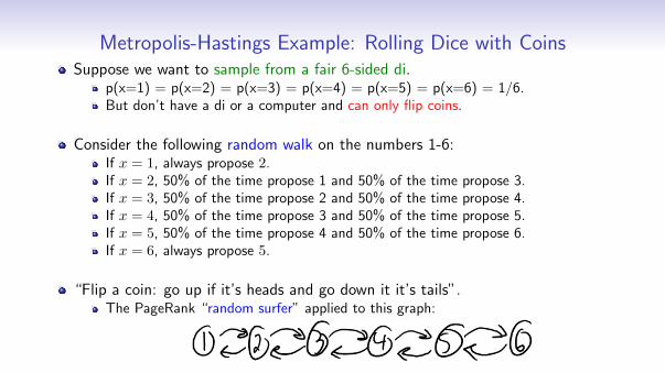
Metropolis-Hastings Example: Rolling Dice with CoinsSuppose we want to sample from a fair 6-sided di.

p(x=1) = p(x=2) = p(x=3) = p(x=4) = p(x=5) = p(x=6) = 1/6.But don’t have a di or a computer and can only flip coins.

Consider the following random walk on the numbers 1-6:If x = 1, always propose 2.If x = 2, 50% of the time propose 1 and 50% of the time propose 3.If x = 3, 50% of the time propose 2 and 50% of the time propose 4.If x = 4, 50% of the time propose 3 and 50% of the time propose 5.If x = 5, 50% of the time propose 4 and 50% of the time propose 6.If x = 6, always propose 5.

“Flip a coin: go up if it’s heads and go down it it’s tails”.The PageRank “random surfer” applied to this graph:

Metropolis-Hastings Example: Rolling Dice with Coins

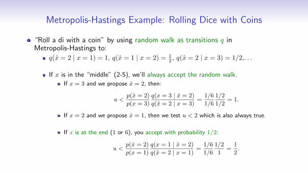
“Roll a di with a coin” by using random walk as transitions q inMetropolis-Hastings to:

q(x̂ = 2 | x = 1) = 1, q(x̂ = 1 | x = 2) = 12 , q(x̂ = 2 | x = 3) = 1/2,. . .

If x is in the “middle” (2-5), we’ll always accept the random walk.

If x = 3 and we propose x̂ = 2, then:

u <p(x̂ = 2)

p(x = 3)

q(x = 3 | x̂ = 2)

q(x̂ = 2 | x = 3)=

1/6

1/6

1/2

1/2= 1.

If x = 2 and we propose x̂ = 1, then we test u < 2 which is also always true.

If x is at the end (1 or 6), you accept with probability 1/2:

u <p(x̂ = 2)

p(x = 1)

q(x = 1 | x̂ = 2)

q(x̂ = 2 | x = 1)=

1/6

1/6

1/2

1=

1

2.

Metropolis-Hastings Example: Rolling Dice with Coins

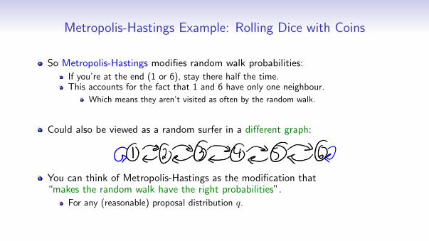
So Metropolis-Hastings modifies random walk probabilities:

If you’re at the end (1 or 6), stay there half the time.This accounts for the fact that 1 and 6 have only one neighbour.

Which means they aren’t visited as often by the random walk.

Could also be viewed as a random surfer in a different graph:

You can think of Metropolis-Hastings as the modification that“makes the random walk have the right probabilities”.

For any (reasonable) proposal distribution q.

Metropolis-Hastings

Simple choices for proposal distribution q:

Metropolis originally used random walks: xt = xt−1 + ε for ε ∼ N (0,Σ).Hastings originally used independent proposal: q(xt | xt−1) = q(xt).Gibbs sampling updates single variable based on conditional:

In this case the acceptance rate is 1 so we never reject.

Mixture model for q: e.g., between big and small moves.“Adaptive MCMC”: tries to update q as we go: needs to be done carefully.“Particle MCMC”: use particle filter to make proposal.

Unlike rejection sampling, we don’t want acceptance rate as high as possible:

High acceptance rate may mean we’re not moving very much.Low acceptance rate definitely means we’re not moving very much.Designing q is an “art”.

Mixture Proposal DistributionMetropolis-Hastings for sampling from mixture of Gaussians:

http://www.cs.ubc.ca/~arnaud/stat535/slides10.pdf

With a random walk q we may get stuck in one mode.

We could have proposal be mixture between random walk and “mode jumping”.

Advanced Monte Carlo Methods

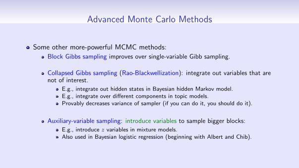
Some other more-powerful MCMC methods:

Block Gibbs sampling improves over single-variable Gibb sampling.

Collapsed Gibbs sampling (Rao-Blackwellization): integrate out variables that arenot of interest.

E.g., integrate out hidden states in Bayesian hidden Markov model.E.g., integrate over different components in topic models.Provably decreases variance of sampler (if you can do it, you should do it).

Auxiliary-variable sampling: introduce variables to sample bigger blocks:

E.g., introduce z variables in mixture models.Also used in Bayesian logistic regression (beginning with Albert and Chib).

Advanced Monte Carlo Methods

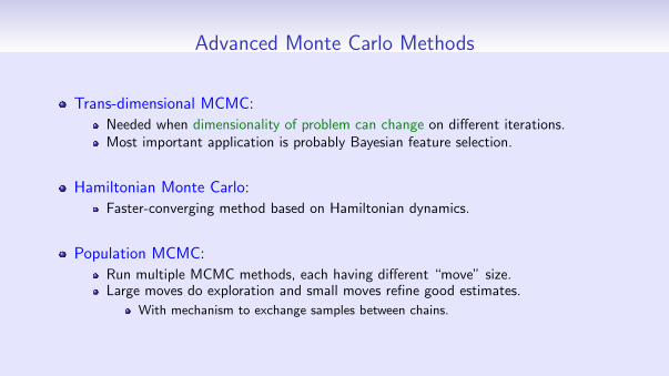
Trans-dimensional MCMC:

Needed when dimensionality of problem can change on different iterations.Most important application is probably Bayesian feature selection.

Hamiltonian Monte Carlo:

Faster-converging method based on Hamiltonian dynamics.

Population MCMC:

Run multiple MCMC methods, each having different “move” size.Large moves do exploration and small moves refine good estimates.

With mechanism to exchange samples between chains.

Summary

Markov chain Monte Carlo generates a sequence of dependent samples:

But asymptotically these samples look like they come from the posterior.

Metropolis-Hastings allows arbitrary “proposals”.

With good proposals works much better than Gibbs sampling.

Next time: generating poetry, music, and dance moves.

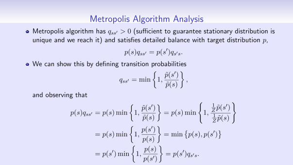
Metropolis Algorithm AnalysisMetropolis algorithm has qss′ > 0 (sufficient to guarantee stationary distribution isunique and we reach it) and satisfies detailed balance with target distribution p,

p(s)qss′ = p(s′)qs′s.

We can show this by defining transition probabilities

qss′ = min

{1,p̃(s′)

p̃(s)

},

and observing that

p(s)qss′ = p(s) min

{1,p̃(s′)

p̃(s)

}= p(s) min

{1,

1Z p̃(s

′)1Z p̃(s)

}

= p(s) min

{1,p(s′)

p(s)

}= min

{p(s), p(s′)

}= p(s′) min

{1,p(s)

p(s′)

}= p(s′)qs′s.