Coverage processes on spheres and condition Burgisser...
37
Coverage processes on spheres and condition numbers for linear programming Burgisser, Peter and Cucker, Felipe and Lotz, Martin 2010 MIMS EPrint: 2012.106 Manchester Institute for Mathematical Sciences School of Mathematics The University of Manchester Reports available from: http://eprints.maths.manchester.ac.uk/ And by contacting: The MIMS Secretary School of Mathematics The University of Manchester Manchester, M13 9PL, UK ISSN 1749-9097
-
Upload
hoangnguyet -
Category
Documents
-
view
212 -
download
0
Transcript of Coverage processes on spheres and condition Burgisser...

Coverage processes on spheres and conditionnumbers for linear programming
Burgisser, Peter and Cucker, Felipe and Lotz, Martin
2010
MIMS EPrint: 2012.106
Manchester Institute for Mathematical SciencesSchool of Mathematics
The University of Manchester
Reports available from: http://eprints.maths.manchester.ac.uk/And by contacting: The MIMS Secretary
School of Mathematics
The University of Manchester
Manchester, M13 9PL, UK
ISSN 1749-9097
arX
iv:0
712.
2816
v3 [
mat
h.PR
] 1
Oct
201
0
The Annals of Probability
2010, Vol. 38, No. 2, 570–604DOI: 10.1214/09-AOP489c© Institute of Mathematical Statistics, 2010
COVERAGE PROCESSES ON SPHERES AND CONDITION
NUMBERS FOR LINEAR PROGRAMMING
By Peter Burgisser1, Felipe Cucker2 and Martin Lotz
University of Paderborn, City University of Hong Kong and OxfordUniversity
This paper has two agendas. Firstly, we exhibit new results forcoverage processes. Let p(n,m,α) be the probability that n sphericalcaps of angular radius α in Sm do not cover the whole sphere Sm.We give an exact formula for p(n,m,α) in the case α ∈ [π/2, π] andan upper bound for p(n,m,α) in the case α ∈ [0, π/2] which tends top(n,m,π/2) when α→ π/2. In the case α ∈ [0, π/2] this yields upperbounds for the expected number of spherical caps of radius α thatare needed to cover Sm.
Secondly, we study the condition number C (A) of the linear pro-gramming feasibility problem ∃x ∈ R
m+1Ax ≤ 0, x 6= 0 where A ∈R
n×(m+1) is randomly chosen according to the standard normal dis-tribution. We exactly determine the distribution of C (A) conditionedto A being feasible and provide an upper bound on the distributionfunction in the infeasible case. Using these results, we show thatE(lnC (A)) ≤ 2 ln(m + 1) + 3.31 for all n > m, the sharpest boundfor this expectancy as of today. Both agendas are related through aresult which translates between coverage and condition.
1. Introduction.
1.1. Coverage processes on spheres.
One of the oldest problems in the theory of coverage processes is that of cal-culating the chance that a given region is completely covered by a sequenceof random sets. Unfortunately there is only a small number of useful circum-stances where this probability may be calculated explicitly. (Hall [13], Section1.11.)
Received April 2008; revised March 2009.1Supported in part by DFG Grant BU 1371/2-1.2Supported in part by CityU GRF Grant CityU 100808.AMS 2000 subject classifications. 60D05, 52A22, 90C05.Key words and phrases. Condition numbers, covering processes, geometric probability,
integral geometry, linear programming.
This is an electronic reprint of the original article published by theInstitute of Mathematical Statistics in The Annals of Probability,2010, Vol. 38, No. 2, 570–604. This reprint differs from the original in paginationand typographic detail.
1
2 P. BURGISSER, F. CUCKER AND M. LOTZ
In 1897 Whitworth [30] considered the following problem. Assume weplace n arcs of angular radius α in the unit circle S1, whose centers areindependently and randomly chosen from the uniform distribution in S1.What is the probability that these arcs do not cover S1?
Whitworth’s problem is arguably at the origin of the theory of coverageprocesses. It was not until 1939 that an answer to the problem was givenwhen Stevens [28] showed that the probability in question is
k∑
j=1
(−1)j+1
(
nj
)(
1− jα
π
)n−1
,(1)
where k = ⌊πα⌋. Extensions of this result to other quantities related with ran-dom arcs in S1 are given in [25]. Extensions to random arcs with differentlengths are given in [9, 16] and in [26] where an exact formula for the prob-ability above is given for randomly placed arcs having random independentsize.
The extension of the original problem in S1 to the two-dimensional unitsphere S2 was considered by Moran and Fazekas de St. Groth [20]. Letp(n,α) denote the probability that n spherical caps of angular radius α, andcenters randomly and independently chosen from the uniform distributionon S2 do not cover S2. Moran and Fazekas de St. Groth exhibited an approx-imation of p(n,α), and numerically estimated this quantity for α = 53◦26′
(a value arising in a biological problem motivating their research). Shortlythereafter, Gilbert [10] showed the bounds
(1− λ)n ≤ p(n,α)≤ 43n(n− 1)λ(1− λ)n−1,(2)
where λ= (sin α2 )
2 = 12(1− cosα) is the fraction of the surface of the sphere
covered by each cap. In addition, Gilbert conjectured that, for n → ∞,p(n,α) satisfies the asymptotic equivalence
p(n,α)≈ n(n− 1)λ2(1− λ2)n−1.
This conjecture was proven by Miles [18] who also found an explicit expres-sion (cf. [17]) for p(n,α) if α ∈ [π/2, π], namely
p(n,α) =
(
n2
)∫ π−α
0sin2(n−2)(θ/2) sin(2θ)dθ
(3)
+3
4
(
n3
)∫ π−α
0sin2(n−3)(θ/2) sin3 θ dθ.
More on the coverage problem for S1 and S2 can be found in [27]. Extensionsof these results to the unit sphere Sm in R
m+1 for m > 2 are scarce. Letp(n,m,α) be the probability that n spherical caps of angular radius α in
COVERAGE PROCESSES AND CONDITION NUMBERS 3
Sm do not cover Sm. That is, for α ∈ [0, π], and a1, . . . , an randomly andindependently chosen points in Sm from the uniform distribution, define
p(n,m,α) := Prob
{
Sm 6=n⋃
i=1
cap(ai, α)
}
,
where cap(a,α) denotes the spherical cap of angular radius α around a. Itcan easily be seen that for n ≤m+ 1 and α≤ π/2 we have p(n,m,α) = 1.Moreover, Wendel [29] has shown that
p(n,m,π/2) = 21−nm∑
k=0
(
n− 1k
)
.(4)
Furthermore, a result by Janson [15] gives an asymptotic estimate of p(n,m,α)for α→ 0. Actually, Janson’s article covers a situation much more generalthan fixed radius caps on a sphere and it was preceded by a paper by Hall[12] where bounds for the coverage probability were shown for the case ofrandom spheres on a torus.
A goal of this paper is to extend some of the known results for S1 andS2 to higher dimensions. To describe our results we first introduce somenotation. We denote by
Om := volm(Sm) =2π(m+1)/2
Γ((m+ 1)/2)
the m-dimensional volume of the sphere Sm. Also, for t ∈ [0,1], denote therelative volume of a cap of radius arccos t ∈ [0, π/2] in Sm by λm(t). It iswell known that
λm(t) =Om−1
Om
∫ arccos t
0(sin θ)m−1 dθ.(5)
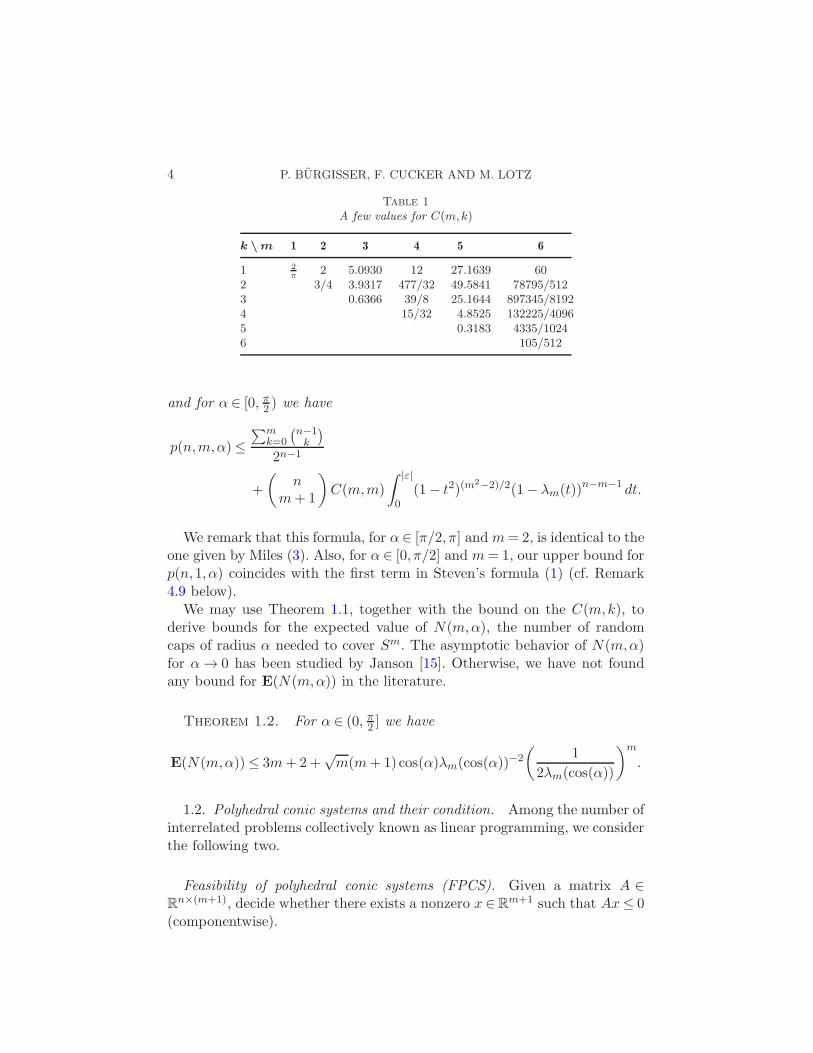
Our results are formulated in terms of a family of numbers C(m,k) definedfor 1 ≤ k ≤ m. These numbers are defined in Section 4.1 and studied inSection 5 where we give bounds on C(m,k) and derive a closed form fork ∈ {1,m− 1,m}. Furthermore, we will show that, for each m, the C(m,k)can be obtained as the solution of a system of linear equations which easilyallows us to produce a table for their values (cf. Table 1).
A main result in this paper is the following.
Theorem 1.1. Let n > m≥ 1, α ∈ [0, π], and ε= cos(π − α). For α ∈[π2 , π]
p(n,m,α) =
m∑
k=1
(
nk+1
)
C(m,k)
∫ 1
εtm−k(1− t2)km/2−1λn−k−1
m (t)dt
4 P. BURGISSER, F. CUCKER AND M. LOTZ
Table 1
A few values for C(m,k)
k \m 1 2 3 4 5 6
1 2π
2 5.0930 12 27.1639 602 3/4 3.9317 477/32 49.5841 78795/5123 0.6366 39/8 25.1644 897345/81924 15/32 4.8525 132225/40965 0.3183 4335/10246 105/512
and for α ∈ [0, π2 ) we have
p(n,m,α)≤∑m
k=0
(n−1k
)
2n−1
+
(
nm+1
)
C(m,m)
∫ |ε|
0(1− t2)(m
2−2)/2(1− λm(t))n−m−1 dt.
We remark that this formula, for α ∈ [π/2, π] andm= 2, is identical to theone given by Miles (3). Also, for α ∈ [0, π/2] and m= 1, our upper bound forp(n,1, α) coincides with the first term in Steven’s formula (1) (cf. Remark4.9 below).
We may use Theorem 1.1, together with the bound on the C(m,k), toderive bounds for the expected value of N(m,α), the number of randomcaps of radius α needed to cover Sm. The asymptotic behavior of N(m,α)for α→ 0 has been studied by Janson [15]. Otherwise, we have not foundany bound for E(N(m,α)) in the literature.
Theorem 1.2. For α ∈ (0, π2 ] we have
E(N(m,α))≤ 3m+2+√m(m+1)cos(α)λm(cos(α))−2
(
1
2λm(cos(α))
)m
.
1.2. Polyhedral conic systems and their condition. Among the number ofinterrelated problems collectively known as linear programming, we considerthe following two.
Feasibility of polyhedral conic systems (FPCS). Given a matrix A ∈Rn×(m+1), decide whether there exists a nonzero x ∈R
m+1 such that Ax≤ 0(componentwise).
COVERAGE PROCESSES AND CONDITION NUMBERS 5
Computation of points in polyhedral cones (CPPC). Given a matrix A ∈Rn×(m+1) such that S = {x ∈R
m+1 |Ax< 0} 6=∅, find x∈ S .
By scaling we may assume without loss of generality that the rows a1, . . . , anof A have Euclidean norm one and interpret the matrix A as a point in(Sm)n. We say that the elements of the set
Fn,m := {A ∈ (Sm)n | ∃x∈ Sm〈a1, x〉 ≤ 0, . . . , 〈an, x〉 ≤ 0},(6)
are feasible. Similarly, we say that the elements in
F◦n,m := {A ∈ (Sm)n | ∃x∈ Sm〈a1, x〉< 0, . . . , 〈an, x〉< 0}(7)
are strictly feasible. Elements in (Sm)n \ Fn,m are called infeasible. Finally,we call ill-posed the elements in Σn,m :=Fn,m \ F◦
n,m.For several iterative algorithms solving the two problems above, it has
been observed that the number of iterations required by an instance A in-creases with the quantity
C (A) =1
dist(A,Σn,m),
(here dist is the distance with respect to an appropriate metric; for the pre-cise definition we refer to Section 2.1). This quantity, known as the GCC-condition number of A [3, 11], occurs together with the dimensions n and min the theoretical analysis (for both complexity and accuracy) of the algo-rithms mentioned above. For example, a primal-dual interior-point methodis used in [6] to solve (FPCS) within
O(√m+ n(ln(m+ n) + lnC (A)))(8)
iterations. The Agmon–Motzkin–Schonberg relaxation method1 [1, 21] orthe perceptron method [23] solve (CPPC) in a number of iterations of orderO(C (A)2) (see Appendix B of [5] for a brief description of this).
The complexity bounds above, however, are of limited use since, unlike nand m, C (A) cannot be directly read from A. A way to remove C (A) fromthese bounds consists in trading worst-case by average-case analysis. To thisend, one endows the space (Sm)n of matrices A with a probability measureand studies C (A) as a random variable with the induced distribution. Inmost of these works, this measure is the unform one in (Sm)n (i.e., matricesA are assumed to have its n rows independently drawn from the uniformdistribution in Sm).
Once a measure has been set on the space of matrices [and in what followswe will assume the uniform measure in (Sm)n], an estimate on E(lnC (A))
1This method gives also the context in which C (A) was first studied, although in thefeasible case only [11].
6 P. BURGISSER, F. CUCKER AND M. LOTZ
yields bounds on the average complexity for (FPCS) directly from (8). For(CPPC) the situation is different since it is known [5], Corollary 9.4, thatE(C (A)2) =∞. Yet, an estimate for ε > 0 on
Prob{C (A)≥ 1/ε |A ∈ Fn,m}yields bounds on the probability that the relaxation or perceptron algorithmswill need more than a given number of iterations. Efforts have therefore beendevoted to compute the expected value (or the distribution function) of C (A)for random matrices A.
Existing results for these efforts are easily summarized. A bound forE(lnC (A)) of the form O(min{n,m lnn}) was shown in [4]. This boundwas improved [7] to max{lnm, ln lnn} + O(1) assuming that n is moder-ately larger than m. Still, in [5], the asymptotic behavior of both C (A)and lnC (A) was exhaustively studied, and these results were extended in[14] to matrices A ∈ (Sm)n drawn from distributions more general than theuniform. Independently of this stream of results, in [8], a smoothed analy-sis for a related condition number is performed from which it follows thatE(lnC (A)) =O(lnn).
Our second set of results adds to the line of research above. First, weprovide the exact distribution of C (A) conditioned to A being feasible anda bound on this distribution for the infeasible case.
Theorem 1.3. Let A ∈ (Sm)n be randomly chosen from the uniformdistribution in (Sm)n, n>m. Then, for ε ∈ (0,1], we have
Prob{C (A)≥ 1/ε |A ∈Fn,m}
=2n−1
∑mk=0
(
n−1k
)
m∑
k=1
(
nk+1
)
C(m,k)
×∫ ε
0tm−k(1− t2)km/2−1λm(t)n−k−1 dt,
Prob{C (A)≥ 1/ε |A /∈Fn,m}
≤ 2n−1
∑n−1k=m+1
(
n−1k
)
(
nm+1
)
C(m,m)
×∫ ε
0(1− t2)(m
2−2)/2(1− λm(t))n−m−1 dt.
Second, we prove an upper bound on E(lnC (A)) that depends only onm, in sharp contrast with all the previous bounds for this expected value.
Theorem 1.4. For matrices A randomly chosen from the uniform dis-tribution in (Sm)n with n>m, we have E(lnC (A))≤ 2 ln(m+ 1) + 3.31.
COVERAGE PROCESSES AND CONDITION NUMBERS 7
Note that the best previously established upper bound for E(lnC (A))(for arbitrary values of n and m) was O(lnn). The bound 2 ln(m+1)+3.31is not only sharper (in that it is independent of n) but also more precise (inthat it does not rely on the O notation).2
1.3. Coverage processes versus condition numbers. Theorems 1.1 and 1.3are not unrelated. Our next result, which will be the first one we will prove,shows a precise link between coverage processes and condition for polyhedralconic systems.
Proposition 1.5. Let a1, . . . , an be randomly chosen from the uniformdistribution in Sm. Denote by A the matrix with rows a1, . . . , an. Then,setting ε := |cos(α)| for α ∈ [0, π], we have
p(n,m,α) =
Prob
{
A ∈Fn,m and C (A)≤ 1
ε
}
, if α ∈ [π/2, π],∑m
k=0
(
n−1k
)
2n−1
+Prob
{
A /∈Fn,m and C (A)≥ 1
ε
}
, if α ∈ [0, π/2].
In particular, p(n,m,π/2) = Prob{A ∈Fn,m}= 21−n∑m
k=0
(
n− 1k
)
.
While Proposition 1.5 provides a dictionary between the coverage prob-lem in the sphere and the condition of polyhedral conic systems, it should benoted that, traditionally, these problems have not been dealt with together.Interest on the second focused on the case of C (A) being large or, equiv-alently, on α being close to π/2. In contrast, research on the first mostlyfocused on asymptotics for either small α or large n (an exception being[29]).
2. Main ideas. In this section we describe in broad strokes how the re-sults presented in the Introduction are arrived at. In a first step in Section2.1, we give a characterization of the GCC condition number which estab-lishes a link to covering problems thus leading to a proof of Proposition 1.5.We then proceed by explaining the main ideas behind the proof of Theorem1.3.
In all that follows, we will write [n] = {1, . . . , n} for n ∈N.
2Recently a different derivation of a O(lnm) bound for E(lnC (A)) was given in [2].However, this derivation does not provide explicit estimates for the constant in the Onotation.
8 P. BURGISSER, F. CUCKER AND M. LOTZ
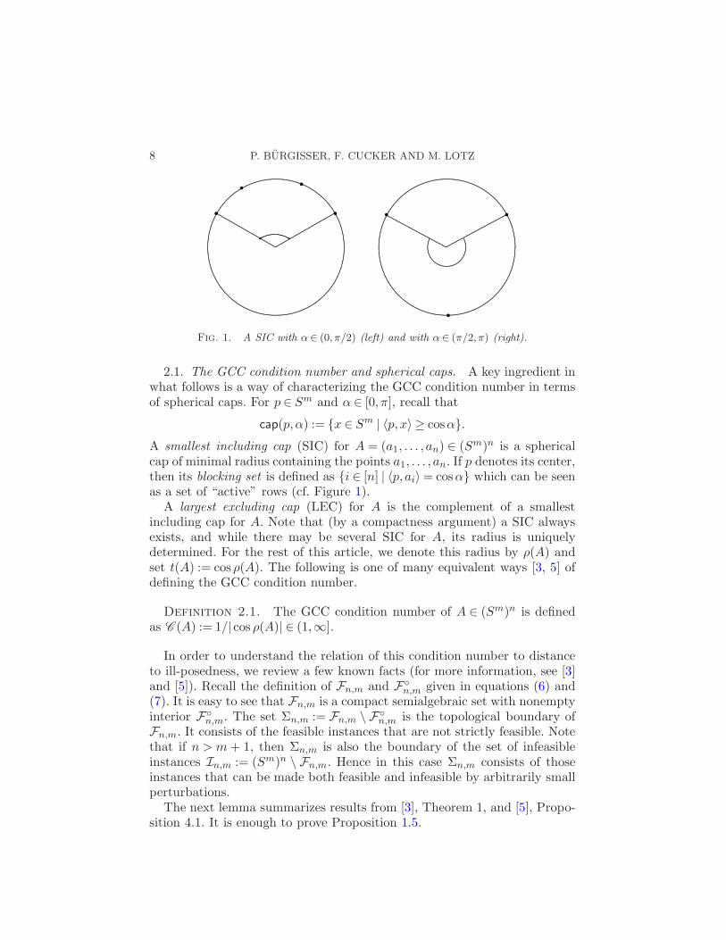
Fig. 1. A SIC with α ∈ (0, π/2) (left) and with α ∈ (π/2, π) (right).
2.1. The GCC condition number and spherical caps. A key ingredient inwhat follows is a way of characterizing the GCC condition number in termsof spherical caps. For p ∈ Sm and α ∈ [0, π], recall that
cap(p,α) := {x ∈ Sm | 〈p,x〉 ≥ cosα}.A smallest including cap (SIC) for A = (a1, . . . , an) ∈ (Sm)n is a sphericalcap of minimal radius containing the points a1, . . . , an. If p denotes its center,then its blocking set is defined as {i ∈ [n] | 〈p, ai〉= cosα} which can be seenas a set of “active” rows (cf. Figure 1).
A largest excluding cap (LEC) for A is the complement of a smallestincluding cap for A. Note that (by a compactness argument) a SIC alwaysexists, and while there may be several SIC for A, its radius is uniquelydetermined. For the rest of this article, we denote this radius by ρ(A) andset t(A) := cos ρ(A). The following is one of many equivalent ways [3, 5] ofdefining the GCC condition number.
Definition 2.1. The GCC condition number of A ∈ (Sm)n is definedas C (A) := 1/| cos ρ(A)| ∈ (1,∞].
In order to understand the relation of this condition number to distanceto ill-posedness, we review a few known facts (for more information, see [3]and [5]). Recall the definition of Fn,m and F◦
n,m given in equations (6) and(7). It is easy to see that Fn,m is a compact semialgebraic set with nonemptyinterior F◦
n,m. The set Σn,m := Fn,m \ F◦n,m is the topological boundary of
Fn,m. It consists of the feasible instances that are not strictly feasible. Notethat if n > m+ 1, then Σn,m is also the boundary of the set of infeasibleinstances In,m := (Sm)n \ Fn,m. Hence in this case Σn,m consists of thoseinstances that can be made both feasible and infeasible by arbitrarily smallperturbations.
The next lemma summarizes results from [3], Theorem 1, and [5], Propo-sition 4.1. It is enough to prove Proposition 1.5.
COVERAGE PROCESSES AND CONDITION NUMBERS 9
Lemma 2.2. We have ρ(A) < π/2 if and only if A ∈ F◦n,m. Moreover,
ρ(A) = π/2 if and only if A ∈Σn,m.
Proof of Proposition 1.5. We claim that
p(n,m,α) = Prob{ρ(A)≤ π−α}.(9)
Indeed,⋃n
i=1 cap(ai, α) 6= Sm iff there exists y ∈ Sm such that y /∈ cap(ai, α)for all i. This is equivalent to ∃y ∀i ai /∈ cap(y,α) which means that an LECfor A has angular radius at least α. This in turn is equivalent to ρ(A)≤ π−αthus proving the claim.
Equation (9) for α= π/2 combined with Lemma 2.2 and Wendel’s result[29] stated in equation (4) yields
21−nm∑
k=0
(
n− 1k
)
= p(n,m,π/2) = Prob{ρ(A)≤ π/2}= Prob{A ∈ Fn,m}.
Suppose now α ∈ [π/2, π]. Then
ρ(A)≤ π− α ⇐⇒ ρ(A)≤ π/2 and C (A)≤ 1
ε,
showing the first assertion of Proposition 1.5. Furthermore, for α ∈ [0, π2 ]
ρ(A)≤ π−α
iff
ρ(A)≤ π/2 or (ρ(A)> π/2 and |cosρ(A)| ≤ |cos(π−α)|),
showing the second assertion of Proposition 1.5. �
2.2. Toward the proof of Theorem 1.3. To prove the feasible case in The-orem 1.3 we note that
Prob
{
C (A)≥ 1
ε
∣
∣
∣A ∈Fn,m
}
=1
volFn,mvolFn,m(ε),
where Fn,m(ε) = {A ∈ F◦n,m | t(A) < ε}. But volFn,m is known by Proposi-
tion 1.5. Therefore, our task is reduced to computing volFn,m(ε). As we willsee in Section 3.1, the smallest including cap SIC(A) is uniquely determinedfor all A ∈ F◦
n,m. Furthermore, for such A, t(A) depends only on the block-ing set of A. Restricting to a suitable open dense subset Rn,m(ε)⊆Fn,m(ε)of “regular” instances, these blocking sets are of cardinality at most m+ 1.This induces a partition
Rn,m(ε) =⋃
I
RIn,m(ε),
10 P. BURGISSER, F. CUCKER AND M. LOTZ
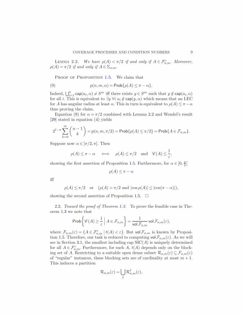
Fig. 2. Determining (a1, a2) ∈ (S2)2 by first giving its span L ∈ G2(R3) and then
ai ∈ S2 ∩L.
where the union is over all subsets I ⊆ [n] of cardinality at most m+1, andRI
n,m(ε) denotes the set of matrices in Rn,m(ε) with blocking set indexed by
I . By symmetry, volRIn,m(ε) only depends on the cardinality of I ; hence it is
enough to focus on computing volR[k+1]n,m (ε) for k = 1, . . . ,m. The orthogonal
invariance and the particular structure of the R[k+1]n,m (ε) (involving certain
convexity conditions) makes possible a change of coordinates that allows oneto split the occurring integral into an integral over t and a quantity C(m,k)that depends only on m and k:
volR[k+1]n,m (ε) =C(m,k)
∫ ε
0g(t, n,m,k)dt.
More precisely, we proceed as follows:
(1) By Fubini, we split the integral over R[k+1]n,m (ε) into an integral over
the first k+1 vectors a1, . . . , ak+1 (determining the blocking set [k+1]) andan integral over ak+2, . . . , an taken from SIC(A):
volR[k+1]n,m (ε) =
∫
A∈R[k+1]k+1,m(ε)
(∫
cap(p(A),ρ(A))n−k−1
d(Sm)n−k−1
)
dR[k+1]k+1,m
(10)
=
∫
A∈R[k+1]k+1,m(ε)
G(A)dR[k+1]k+1,m.
This is an integral of the function G(A) := vol(cap(p(A), ρ(A)))n−k−1 whichis a certain power of the volume of the spherical cap SIC(A).
(2) The next idea is to specify A = (a1, . . . , ak+1) in R[k+1]k+1,m(ε) by first
specifying the subspace L spanned by these vectors and then the positionof the ai on the sphere Sm ∩L∼= Sk (cf. Figure 2).
Let Gk+1(Rm+1) denote the Grassmann manifold of (k + 1)-dimensional
subspaces in Rm+1 and consider the map
R[k+1]k+1,m(ε)→Gk+1(R
m+1),
COVERAGE PROCESSES AND CONDITION NUMBERS 11
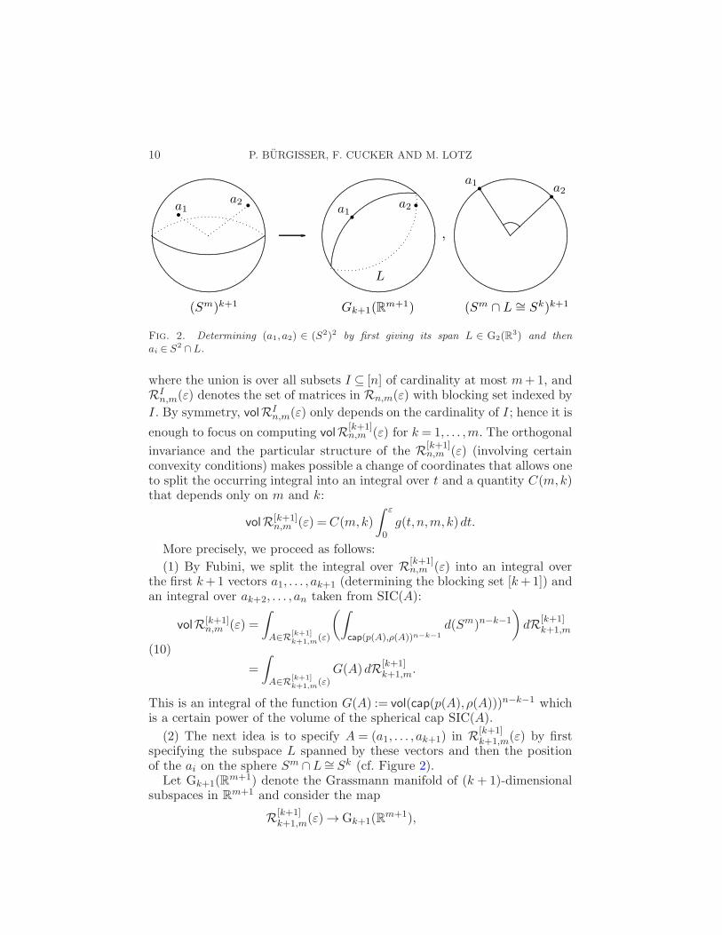
Fig. 3. Determining (a1, a2, a3) ∈ (S2)3 by specifying the direction p, the height t, andthe ai on the subsphere {a ∈ S2 | 〈a, p〉= t} by bi.
(11)(a1, . . . , ak+1) 7→ L= span{a1, . . . , ak+1}.
Clearly, a vector a ∈ Sm lies in the special subspace L0 :=Rk+1× 0 iff it lies
in the subsphere Sk. Hence the fibre over L0 consists of all “regular” tuplesA= (a1, . . . , ak+1) ∈ (Sk)k+1 such that t(A)< ε, and hence the fibre can be
identified with R[k+1]k+1,k(ε). Using the orthogonal invariance and the coarea
formula (also called Fubini’s theorem for Riemannian manifolds) we canreduce the computation of the integral (10) to an integral over the special
fibre R[k+1]k+1,k(ε). This leads to
∫
R[k+1]k+1,m(ε)
G(A)dR[k+1]k+1,m = volGk+1(R
m+1)
∫
R[k+1]k+1,k(ε)
G(A)J(A)dR[k+1]k+1,k ,
where J(A) is the normal Jacobian of the transformation (11).(3) To specify a regular A= (a1, . . . , ak+1) ∈ (Sk)k+1, we first specify the
direction p= p(A) ∈ Sk and the height t= t(A) ∈ (0, ε) and then the positionof the ai on the subsphere {a ∈ Sk | 〈a, p〉= t} ≃ Sk−1 (cf. Figure 3).
More precisely, we consider the map
R[k+1]k+1,k(ε)→ Sk × (0, ε), A 7→ (p(A), t(A)).(12)
The fibre over (p0, t), where p0 = (0, . . . ,0,1) is the “north pole,” consists oftuples (a1, . . . , ak+1) lying on the “parallel” subsphere {a ∈ Sk | 〈a, p〉= t}.The vectors ai can be described by points bi ∈ Sk−1, which are obtained byprojecting ai orthogonally onto R
k × 0 and scaling the resulting vector tolength one.
The orthogonal invariance and the coarea formula allow us to reduce the
computation of the integral over R[k+1]k+1,k(ε) to the integration over t ∈ [0, ε] of
an integral over the special fibres over (p0, t). The latter integral is capturedby the coefficient C(m,k) which can be interpreted as a higher moment of
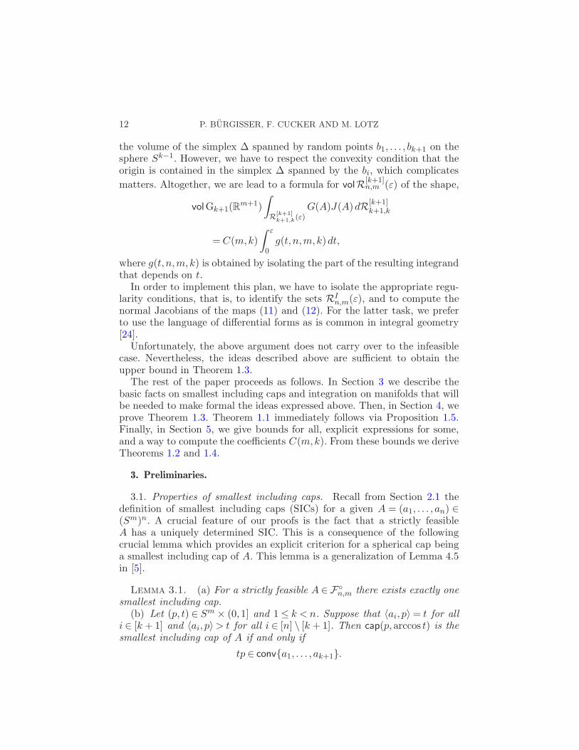
12 P. BURGISSER, F. CUCKER AND M. LOTZ
the volume of the simplex ∆ spanned by random points b1, . . . , bk+1 on thesphere Sk−1. However, we have to respect the convexity condition that theorigin is contained in the simplex ∆ spanned by the bi, which complicates
matters. Altogether, we are lead to a formula for volR[k+1]n,m (ε) of the shape,
volGk+1(Rm+1)
∫
R[k+1]k+1,k(ε)
G(A)J(A)dR[k+1]k+1,k
=C(m,k)
∫ ε
0g(t, n,m,k)dt,
where g(t, n,m,k) is obtained by isolating the part of the resulting integrandthat depends on t.
In order to implement this plan, we have to isolate the appropriate regu-larity conditions, that is, to identify the sets RI
n,m(ε), and to compute thenormal Jacobians of the maps (11) and (12). For the latter task, we preferto use the language of differential forms as is common in integral geometry[24].
Unfortunately, the above argument does not carry over to the infeasiblecase. Nevertheless, the ideas described above are sufficient to obtain theupper bound in Theorem 1.3.
The rest of the paper proceeds as follows. In Section 3 we describe thebasic facts on smallest including caps and integration on manifolds that willbe needed to make formal the ideas expressed above. Then, in Section 4, weprove Theorem 1.3. Theorem 1.1 immediately follows via Proposition 1.5.Finally, in Section 5, we give bounds for all, explicit expressions for some,and a way to compute the coefficients C(m,k). From these bounds we deriveTheorems 1.2 and 1.4.
3. Preliminaries.
3.1. Properties of smallest including caps. Recall from Section 2.1 thedefinition of smallest including caps (SICs) for a given A = (a1, . . . , an) ∈(Sm)n. A crucial feature of our proofs is the fact that a strictly feasibleA has a uniquely determined SIC. This is a consequence of the followingcrucial lemma which provides an explicit criterion for a spherical cap beinga smallest including cap of A. This lemma is a generalization of Lemma 4.5in [5].
Lemma 3.1. (a) For a strictly feasible A ∈ F◦n,m there exists exactly one
smallest including cap.(b) Let (p, t) ∈ Sm × (0,1] and 1≤ k < n. Suppose that 〈ai, p〉= t for all
i ∈ [k + 1] and 〈ai, p〉> t for all i ∈ [n] \ [k + 1]. Then cap(p,arccos t) is thesmallest including cap of A if and only if
tp ∈ conv{a1, . . . , ak+1}.
COVERAGE PROCESSES AND CONDITION NUMBERS 13
Proof. We first show that assertion (b) implies assertion (a). Supposecap(p1, ρ) and cap(p2, ρ) are SICs for A, and put t := cos ρ. Note that t > 0.Assertion (b) implies that tp1 is contained in the convex hull of a1, . . . , an;hence there exist λi ≥ 0 such that
∑
i λi = 1 and tp1 =∑
i λiai. Therefore,〈tp1, p2〉=
∑
i λi〈ai, p2〉 ≥ t, as 〈ai, p2〉 ≥ t for all i. This implies 〈p1, p2〉 ≥ 1and hence p1 = p2.
The proof of assertion (b) goes along the lines of Lemma 4.5 in [5]. Supposefirst that cap(p,α) is a SIC for A where α := arccos t. It is sufficient toshow that p ∈ cone{a1, . . . , ak+1}. Indeed, if p =
∑
λiai with λi ≥ 0, thentp =
∑
(tλi)ai. Furthermore,∑
(tλi) =∑
λi〈ai, p〉= 〈∑λiai, p〉= ‖p‖2 = 1.Hence tp ∈ conv{a1, . . . , ak+1}.
We now argue by contradiction: if p is not contained in cone{a1, . . . , ak+1},then there exists a vector v ∈ Sm such that 〈p, v〉< 0 and 〈ai, v〉> 0 for alli ∈ {1, . . . , k+ 1}. For δ > 0 we set
pδ :=p+ δv
‖p+ δv‖ =p+ δv
√
1 + 2δ〈p, v〉+ δ2.(13)
Then for 1≤ i≤ k+ 1 and sufficiently small δ we have
〈ai, pδ〉=t+ δ〈ai, v〉
√
1 + 2δ〈p, v〉+ δ2> t,
where we used that 〈ai, p〉= t, 〈ai, v〉> 0 and 〈p, v〉< 0.For k+2≤ i≤ n the function δ→ 〈ai, pδ〉 is continuous at δ = 0. Since, by
hypothesis, 〈ai, p〉= 〈ai, p0〉 > t, it follows that 〈ai, pδ〉> t for δ sufficientlysmall. From this we conclude that for sufficiently small δ there exists tδ > tsuch that 〈ai, pδ〉 > tδ for all i ∈ [n]. Setting αδ = arccos tδ we obtain thatαδ < α and ai ∈ cap(pδ, αδ) for all i ∈ [n], contradicting the assumption thatcap(p,α) is a smallest including cap.
To prove the other direction, we suppose tp ∈ conv{a1, . . . , ak+1}. For q ∈Sm let α(q) we denote the angular radius of the smallest spherical cap withcenter q containing a1, . . . , an. If we assume that cap(p,α) is not a SIC forA, then there exists a vector v ∈ Sm and δ0 > 0, such that 〈v, p〉 = 0 and,
for all 0< δ ≤ δ0, α(pδ)<α(p) where pδ =p+δv√1+δ2
(i.e., we have a direction v
along which we can move to obtain a smaller cap). This means that
min1≤i≤n
〈ai, pδ〉> min1≤i≤n
〈ai, p〉= t.
Therefore, for all i ∈ [k+1] we have
〈ai, pδ〉=〈ai, p〉+ δ〈ai, v〉√
1 + δ2> t= 〈ai, p〉
14 P. BURGISSER, F. CUCKER AND M. LOTZ
for sufficiently small δ which implies that 〈ai, v〉> 0. Let µ ∈ Rk+1≥0 be such
that tp=∑
1≤i≤k+1 µiai and∑
1≤i≤k+1µi = 1. Then we have
t〈p, v〉=∑
1≤i≤k+1
µi〈ai, v〉> 0,
contradicting the assumption that 〈p, v〉 = 0. Thus cap(p,α) is indeed asmallest including cap. �
For a strictly feasible A, we denote the center of its uniquely determinedSIC by p(A) and its radius by ρ(A). The blocking set BS(A) of A is definedas the blocking set of the SIC of A. It is not hard to see that BS(A) canhave any cardinality greater than one.
However, we note that in the infeasible case, there may be more than onesmallest including cap. Consider for instance three equilateral points on thecircle (right-hand side in Figure 1). It is known [5], Proposition 4.2, thatin this case, the blocking set of a SIC has at least m+ 1 elements. In theinfeasible case, one direction of the characterization of smallest includingcaps of Lemma 3.1 still holds. The proof is similar as for Lemma 3.1.
Lemma 3.2. Let cap(p,arccos t) be a SIC for A ∈ (Sm)n with p ∈ Sm
and t ∈ (−1,0). Suppose 〈ai, p〉 = t for i ∈ [m + 1] and 〈ai, p〉 > t for i =m+2, . . . , n. Then tp ∈ conv{a1, . . . , am+1}.
Proof. Suppose tp /∈ conv{a1, . . . , am+1}. Then−p /∈ cone{a1, . . . , am+1}and hence there exists a vector v ∈ Sm such that 〈−p, v〉< 0 and 〈ai, v〉> 0for all i. For δ > 0 we define pδ as in (13). Take δ sufficiently small so thatt < t+ δ〈ai, v〉< 0 for all i ∈ [m+1]. Then, for i ∈ [m+1] and δ sufficientlysmall, we have
〈ai, pδ〉=t+ δ〈ai, v〉
√
1 + 2δ〈p, v〉+ δ2> t,
where we used that 〈ai, p〉 = t, 〈ai, v〉 > 0, and 〈p, v〉 > 0. This shows thatcap(p,arccos t) is not a smallest including cap. �
We present a few more auxiliary results that are needed for the proof ofour main result.
Lemma 3.3. For given linearly independent a1, . . . , ak+1 ∈ Sm, 1≤ k ≤m, there exist unique p ∈ Sm and t ∈ (0,1) such that
p ∈ span{a1, . . . , ak+1}and
〈ai, p〉= t for all i ∈ [k +1].
Moreover, the map (a1, . . . , ak+1) 7→ (p, t) is differentiable.
COVERAGE PROCESSES AND CONDITION NUMBERS 15
Proof. Let A denote the affine span of a1, . . . , ak+1, L the underlyinglinear space and L the linear span of A. Since the ai are linearly indepen-dent, we have A 6= L and thus dimA= dimL= k, dimL= k+1. Hence theintersection of L with the orthogonal complement L⊥ is one-dimensionaland contains exactly two elements of length one. Take the one such that thecommon value t= 〈ai, p〉 is positive. This shows existence and at the sametime the uniqueness of p, t.
Suppose now k =m, and let A denote the square matrix with the rowsa1, . . . , am+1. The conditions 〈ai, p〉 = t can be written in matrix form asAp = te where e := (1, . . . ,1)⊤. By solving this equation we obtain the fol-lowing explicit formulas:
p(A) =1
‖A−1e‖A−1e, t(A) =
1
‖A−1e‖ .(14)
This shows the differentiability of the map A 7→ (p, t) in the case k =m. Weleave the proof in the general case to the reader. �
The next result, though very elementary, will be useful for clarification.Let p ∈ Sk and t 6= 0 and consider elements a1, . . . , ak+1 ∈ Sk satisfying
〈ai, p〉= t for all i. Let bi ∈ Sk−1 be the scaled-to-one orthogonal projectionof ai onto the orthogonal complement of Rp. That is, ai = rbi + tp wherer = (1− t2)1/2.
Lemma 3.4. The following conditions are equivalent:
1. The affine hull A of a1, . . . , ak+1 has dimension k.2. The span of b1, . . . , bk+1 has dimension k.3. a1, . . . , ak+1 are linearly independent.
Proof. The equivalence of the first two conditions is obvious. Theequivalence of the first and third condition follows from dim span(A) =dimA+1 (here we use t 6= 0). �
3.2. Volume forms on Grassmann manifolds. Integration on Grassmannmanifolds will play a crucial role in our proofs. We recall some facts aboutthe relevant techniques from integral geometry and refer to Santalo’s book[24], II.9–12, and the article [19] for more information. We recall that volumeelements are always unsigned forms.
Let M be a Riemannian manifold of dimension m, p ∈M , and let y =(y1, . . . , ym)⊤ :U 7→ R
m be local coordinates in a neighborhood U of p suchthat ∂/∂y1, . . . , ∂/∂ym are an orthonormal basis of TpM . The natural volumeform on M at p associated to its Riemannian metric is then given by dM =dy1 ∧ · · · ∧ dym where dyi is the differential of the coordinate function yi atp.
16 P. BURGISSER, F. CUCKER AND M. LOTZ
In the case of a sphere, we get such local coordinates around a pointp ∈ Sm by projecting onto the orthogonal complement of p. More pre-cisely, let 〈e1, . . . , em+1〉 be an orthonormal basis of Rm+1 satisfying e1 =p (so that e2, . . . , em+1 span the tangent space TpS
m). For a point x =(x1, . . . , xm+1)
⊤ ∈ Sm in a neighbourhood of p set yi = 〈x, ei〉. Then (y2, . . . ,ym+1) are local coordinates of Sm around p such that ∂/∂yi are pairwiseorthogonal at p. Hence the volume element of Sm at p is given by
dSm = ω2 ∧ · · · ∧ ωm+1,
where ωi := dyi = 〈dx, ei〉 and dx= (dx1, . . . , dxm+1)⊤. Hence, if we denote
by E the (m + 1) × (m + 1)-matrix having the ei as rows, we obtain thevolume form by wedging the nonzero entries of E dx.
In a similar fashion we define volume forms on Stiefel manifolds (for detailsand further justification we refer to [24]). A k-frame is a set of k linearly inde-pendent vectors. For 1≤ k ≤m+1, the Stiefel manifold Vk(R
m+1) is definedas the set of orthonormal k-frames in R
m+1. It is a compact Riemanniansubmanifold of (Sm)k. Let Q= (q1, . . . , qk) ∈ Vk(Rm+1) and 〈e1, . . . , em+1〉 anorthonormal basis of Rm+1 such that e1 = q1, . . . , ek = qk. Then the volumeelement of Vk(R
m+1) at Q is given by
dVk(Rm+1) =
∧
1≤i≤k
(ωi,i+1 ∧ · · · ∧ ωi,m+1),
where ωi,j = 〈dqi, ej〉 for 1≤ i≤ k and 1≤ j ≤m+ 1. [In terms of the (m+1)× k matrix E dQ, this corresponds to wedging the entries below the maindiagonal.] With this volume element we have volVk(R
m+1) =Om · · ·Om+1−k.We denote by Gk(R
m+1) the Grassmann manifold of k-dimensional sub-spaces of Rm+1. One way of characterizing it is as a quotient of a Stiefel man-ifold, by identifying frames that span the same subspace. Let L ∈Gk(R
m+1)and choose a frame Q ∈ Vk(Rm+1) spanning L. If Vk(L) denotes the Stiefelmanifold of orthonormal k-frames in L and dVk(L) its volume element atQ, then it is known that the volume element dGk(R
m+1) of the Grassmannmanifold at L satisfies (see [19], equation (10))
dVk(Rm+1) = dGk(R
m+1)∧ dVk(L).(15)
From this equality it follows that
dGk(Rm+1) =
∧
1≤i≤k
(ωi,k+1 ∧ · · · ∧ ωi,m+1)
with the ωi,j as defined in the case of the Stiefel manifold. (In terms ofthe matrix EdQ, this corresponds to wedging the elements in the lower(m + 1 − k) × k rectangle.) As a consequence of (15), the volume of theGrassmannian is given by
Gk,m+1 := volGk(Rm+1) =
Om+1−k · · ·Om
O0 · · ·Ok−1.
COVERAGE PROCESSES AND CONDITION NUMBERS 17
Equation (15) has a generalization to frames that are not orthogonal,that is, to points in a product of spheres (Sm)k. Let L ∈ Gk(R
m+1) andset S(L) := L ∩ Sm, so that S(L) ∼= Sk−1. Choose a basis a1, . . . , ak of Lconsisting of unit length vectors, that is, a point A= (a1, . . . , ak) in S(L)
k.We denote by vol(A) the volume of the parallelepiped spanned by the ai.Then the volume form of (Sm)k at A can be expressed as
d(Sm)k = vol(A)m−k+1 dGk(Rm+1)∧ dS(L)k.(16)
This equation can be derived as in [19] (see also [24], II.12.3). It also followsas a special case of a general formula of Blaschke–Petkantschin-type derivedby Zahle [31] (see also the discussion in [22]).
A beautiful application of equation (16) is that it allows an easy compu-tation of the moments of the absolute values of random determinants. Thefollowing lemma is an immediate consequence of (16) (see also [19]).
Lemma 3.5. Let B ∈ (Sk)k+1 be a matrix with rows b1, . . . , bk indepen-dently and uniformly distributed in Sk. Then
E(|det(B)|m−k+1) =
( Om
Ok−1
)k 1
Gk,m+1.
4. The probability distribution of C (A). This section is devoted to theproof of Theorem 1.3.
4.1. The feasible case. Recall that, for A ∈ F◦n,m, we denote the center
and the angular radius of the unique smallest including cap of A by p(A)and ρ(A), respectively, and we write t(A) = cosρ(A).
Our goal here is to prove the first part of Theorem 1.3, for which, as wenoted in Section 2.2, we just need to compute the volume of the followingsets:
Fn,m(ε) := {A ∈ F◦n,m | t(A)< ε}.
For this purpose it will be convenient to decompose Fn,m(ε) according to thesize of the blocking sets. Recall that the blocking set of A ∈ F◦
n,m is definedas
BS(A) = {i ∈ [n] | 〈p(A), ai〉= t(A)}.(17)
For I ⊆ [n] with |I| ≤ n and ε ∈ (0,1] we define FIn,m(ε) to be the set of all
A ∈ Fn,m(ε) such that BS(A) = I .For technical reasons we have to require some regularity conditions for
the elements of FIn,m(ε).
18 P. BURGISSER, F. CUCKER AND M. LOTZ
Definition 4.1. We call a family (a1, . . . , ak+1) of elements of a vectorspace centered with respect to a vector c in the affine hull A of the ai ifdimA= k, and c lies in the relative interior of the convex hull of the ai. Wecall the family centered if it is centered with respect to the origin. We nowdefine, for I ⊆ [n],
RIn,m(ε) := {A ∈FI
n,m(ε) | (ai)i∈I is centered with respect to t(A)p(A)}.
Note that, by definition, the ai are affinely independent if |I| ≤m+1.
Lemma 4.2. 1. FIn,m(ε) is of measure zero if |I|>m+ 1.
2. If |I| ≤m+1, then RIn,m(ε) is open in (Sm)n, and FI
n,m(ε) is contained
in the closure of RIn,m(ε).
3. FIn,m(ε) \RI
n,m(ε) has measure zero.
Proof. 1. If A ∈FIn,m(ε), then {ai | i ∈ I} is contained in the boundary
of the SIC of A, and hence its affine hull has dimension at most m. On theother hand, the affine hull of (ai)i∈I is almost surely R
m+1 if |I|>m+ 1.2. The fact that RI
n,m(ε) is open in (Sm)n easily follows from the conti-nuity of the map A 7→ (p(A), t(A)) established in Lemma 3.3.
Suppose now A ∈ FIn,m(ε). By Lemma 3.1 we have t(A)p(A) ∈ conv{ai |
i ∈ I} for A ∈ FIn,m(ε). It is now easy to see that there are elements A′
arbitrarily close to A such that A′ is centered with respect to t(A′)p(A′).This shows the second assertion.
3. By part two we haveRIn,m(ε)⊆FI
n,m(ε)⊆RIn,m(ε). Since we are dealing
with semialgebraic sets, the boundary of RIn,m(ε) is of measure zero. �
It is clear that the FIn,m with I of the same cardinality just differ by a
permutation of the vectors. Using Lemma 4.2 we obtain
volFn,m(ε) =∑
|I|≤m+1
volFIn,m(ε) =
m∑
k=1
(
nk+1
)
volRkn,m(ε),(18)
where we have put Rkn,m(ε) :=R[k+1]
n,m (ε) to ease notation.
Hence it is sufficient to compute the volume of Rkn,m(ε). For this purpose
we introduce now the coefficients C(m,k).
Definition 4.3. We define for 1≤ k ≤m
C(m,k) =(k!)m−k+1
Okm
Gk,m
∫
Mk
(volk∆)m−k+1 d(Sk−1)k+1,
COVERAGE PROCESSES AND CONDITION NUMBERS 19
where Mk is the following open subset of Sk−1:
Mk := {(b1, . . . , bk+1) ∈ (Sk−1)k+1 | (b1, . . . , bk+1) is centered}
and ∆ :Mk →R maps B = (b1, . . . , bk+1) to the convex hull of the bi.
Example 4.4. We compute C(m,1). Note thatM1,1 = {(−1,1), (1,−1)}and G1,m = 1
2Om−1. Hence
C(m,1) =1
Om
1
2Om−1
∫
M1,1
(vol1∆)m dM1,1 =Om−1
Om2m.
The assertion in Theorem 1.3 about the feasible case follows immediatelyfrom Proposition 1.5, equation (18) and the following result.
Proposition 4.5. Let ε ∈ (0,1]. The relative volume of Fkn,m(ε) is given
by
volRkn,m(ε)
Onm
=C(m,k)
∫ ε
0tm−k(1− t2)km/2−1λm(t)n−k−1 dt.
Proof. Consider the projection
Rkn,m(ε)→Rk
k+1,m(ε), (a1, . . . , an) 7→A= (a1, . . . , ak+1).
By Lemma 3.1, this map is surjective and its fiber over A consists of all(A,ak+2, . . . , an) such that ai lies in the interior of the cap cap(p(A), ρ(A))for all i > k+ 1. By Fubini, and using (5), we conclude that
volRkn,m(ε)
On−k−1m
=
∫
A∈Rkk+1,m(ε)
λm(t(A))n−k−1 d(Sm)k+1.(19)
We consider now the following map (which is well defined [cf. Lemma 3.4]):
Rkk+1,m(ε)→Gk+1(R
m+1), (a1, . . . , ak+1) 7→ L= span{a1, . . . , ak+1}.
We can thus integrate overRkk+1,m(ε) by first integrating over L ∈Gk+1(R
m+1)
and then over the fiber of L. By equation (16), the volume form of (Sm)k+1
at A can be written as
d(Sm)k+1 = vol(A)m−k dGk+1(Rm+1)(L)∧ dS(L)k+1,
where S(L)k+1 denotes (k + 1)-fold product of the unit sphere of L. Byinvariance under orthogonal transformations, the integral over the fiber doesnot depend on L. We may therefore assume that L = R
k+1, in which case
20 P. BURGISSER, F. CUCKER AND M. LOTZ
the fiber over L can be identified with Rkk+1,k(ε). Thus we conclude from
equation (19) that
volRkn,m(ε)
On−k−1m
= Gk+1,m+1
∫
A∈Rkk+1,k(ε)
vol(A)m−kλm(t(A))n−k−1 d(Sk)k+1.(20)
In a next step, we will perform a change of variables in order to expressthe integral on the right-hand side of equation (20) as an integral over tinvolving the coefficients C(m,k).
Note that by Lemma 3.3, p(A) ∈ Sk and t(A) ∈ (0,1) are defined for anyA ∈GL(k+1,R) and depend smoothly on A. A moment’s thought (togetherwith Lemmas 3.1 and 3.4) shows that we have the following complete char-acterization of Rk
k+1,k(ε):
Rkk+1,k(ε) = {A ∈ (Sk)k+1 |A is centered with respect to t(A)p(A),
0< t(A)< ε,∀i 〈ai, p(A)〉= t(A)}.
For A ∈ Rkk+1,k(ε) set p := p(A), t := t(A), and r := r(t) := (1− t2)1/2. For
i ∈ [k+1] we define bi as the scaled-to-one orthogonal projection of ai ontothe orthogonal complement of Rp, briefly ai = rbi+tp. The matrix B =B(A)with the rows b1, . . . , bk+1 can be written as B = 1
r (A− tep⊤). Clearly, B iscentered.
We define now
Wk = {(B,p) ∈ (Sk)k+1 × Sk |Bp= 0 and B is centered}.
This is a Riemannian submanifold of (Sk)k+2 of dimension k(k+1)− 1. Wethus have a map,
ϕk :Rkk+1,k(ε)→Wk × (0, ε), A 7→ (B(a), p(A), t(A)).
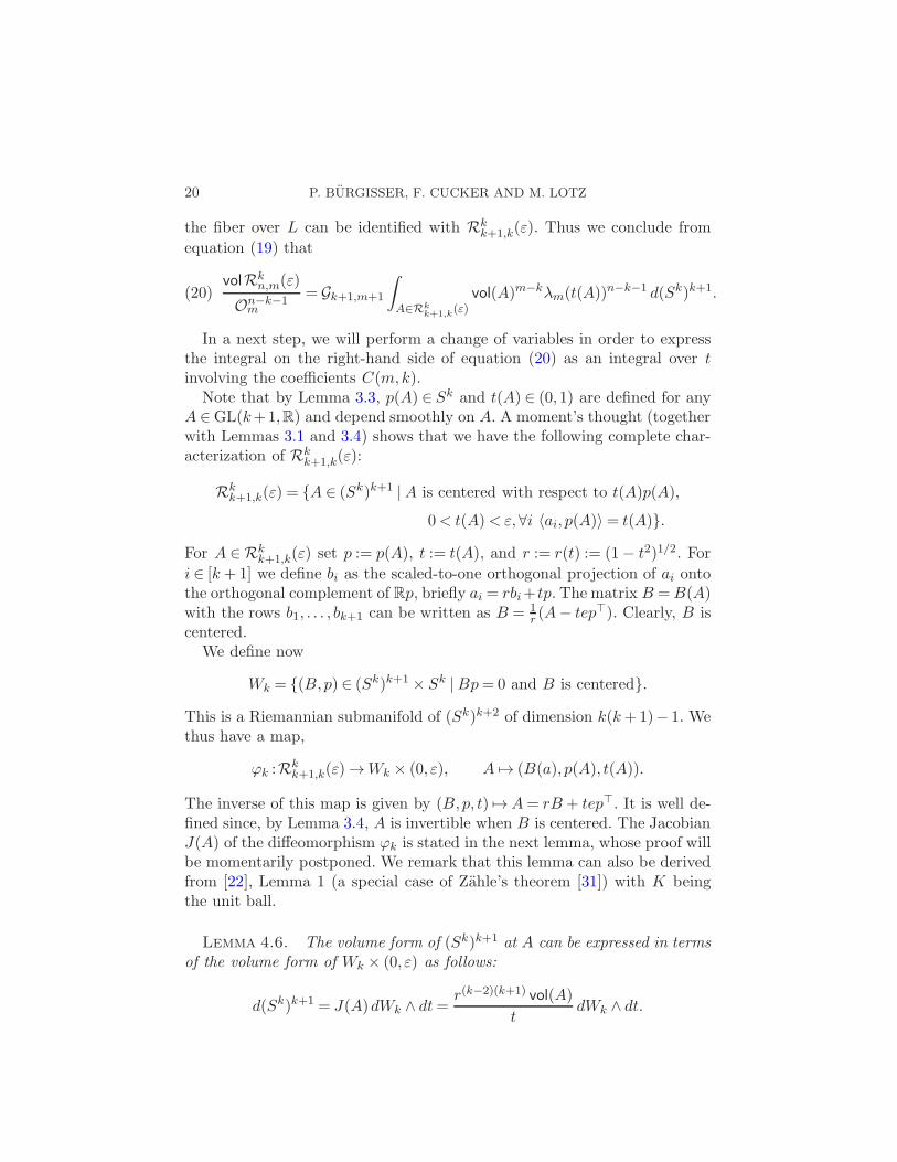
The inverse of this map is given by (B,p, t) 7→A= rB + tep⊤. It is well de-fined since, by Lemma 3.4, A is invertible when B is centered. The JacobianJ(A) of the diffeomorphism ϕk is stated in the next lemma, whose proof willbe momentarily postponed. We remark that this lemma can also be derivedfrom [22], Lemma 1 (a special case of Zahle’s theorem [31]) with K beingthe unit ball.
Lemma 4.6. The volume form of (Sk)k+1 at A can be expressed in termsof the volume form of Wk × (0, ε) as follows:
d(Sk)k+1 = J(A)dWk ∧ dt=r(k−2)(k+1) vol(A)
tdWk ∧ dt.
COVERAGE PROCESSES AND CONDITION NUMBERS 21
We now express the Jacobian J(A) in terms of (B,p, t). The volume vol(A)of the parallelepiped spanned by the ai equals (k +1)! times the volume ofthe pyramid with apex 0 and base ∆(a1, . . . , ak+1), the latter denoting thesimplex with vertices a1, . . . , ak+1. Moreover, this pyramid has height t andit is well known that the volume of a (k + 1)-dimensional pyramid withheight t and base B is t
k+1 times the (k-dimensional) volume of B. Thisimplies
vol(A) = (k +1)!t
k +1volk−1∆(rb1, . . . , rbk+1) = k!rkt volk∆(B).
From this expression, together with (20), we conclude that
volRkn,m(ε)
Onm
=Gk+1,m+1
Ok+1m
∫
Wk×(0,ε)vol(A)m−k+1 r(t)
(k−2)(k+1)
t
× λm(t)n−k−1 d(Sk)k+1
=Gk+1,m+1(k!)
m−k+1
Ok+1m
∫
Wk
volk∆(B)m−k+1 dWk
×∫ ε
0tm−kr(t)km−2λm(t)n−k−1 dt.
Consider the projection pr :Wk → Sk, (B,p) 7→ p. We note that its fiberover p can be identified with the set Mk (cf. Definition 4.3). By the in-variance of volk∆(B) under rotation of p ∈ Sk, we get
∫
Wk
volk∆(B)m−k+1 dWk =Ok
∫
Mk
volk∆(B)m−k+1 d(Sk−1)k+1.
Note that, up to a scaling factor, the right-hand side above is the coefficientC(m,k) introduced in Definition 4.3. Using (Ok/Om)Gk+1,m+1 = Gk,m weobtain
volRkn,m(ε)
Onm
=C(m,k)
∫ ε
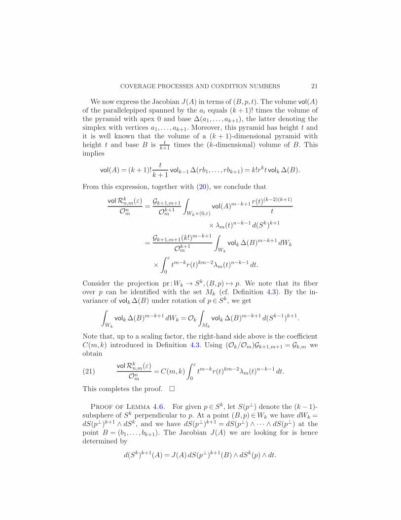
0tm−kr(t)km−2λm(t)n−k−1 dt.(21)
This completes the proof. �
Proof of Lemma 4.6. For given p ∈ Sk, let S(p⊥) denote the (k− 1)-subsphere of Sk perpendicular to p. At a point (B,p) ∈Wk we have dWk =dS(p⊥)k+1 ∧ dSk, and we have dS(p⊥)k+1 = dS(p⊥) ∧ · · · ∧ dS(p⊥) at thepoint B = (b1, . . . , bk+1). The Jacobian J(A) we are looking for is hencedetermined by
d(Sk)k+1(A) = J(A)dS(p⊥)k+1(B)∧ dSk(p)∧ dt.
22 P. BURGISSER, F. CUCKER AND M. LOTZ
Choose an orthonormal moving frame e1, . . . , ek, ek+1 with p(A) = ek+1.For 1 ≤ i ≤ k define the one-forms µi := −〈ei, dp〉 (compare Section 3.2).Then the volume form of Sk at p is given by dSk(p) = µ1 ∧ · · · ∧ µk.
Differentiating te = Ap we get edt = dAp + Adp. By multiplying bothsides with A−1 and using formula (14) we obtain
p(dt/t)− dp=A−1 dAp.
Let Q denote the (k+1)× (k+1) matrix having the ei as rows. With respectto this basis, the above equation takes the form
(µ1, . . . , µk, dt/t)⊤ =Q(p(dt/t)− dp) =QA−1 dAp.(22)
Wedging the entries on both sides yields
dSk(p)∧ dt= t vol(A)−1〈p, da1〉 ∧ · · · ∧ 〈p, dak+1〉.(23)
The volume form of S(p⊥) at bi is given by
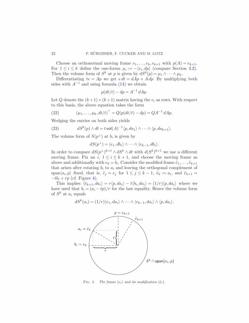
dS(p⊥) = 〈e1, dbi〉 ∧ · · · ∧ 〈ek−1, dbi〉.In order to compare dS(p⊥)k+1 ∧ dSk ∧ dt with d(Sk)k+1 we use a differentmoving frame. Fix an i, 1 ≤ i ≤ k + 1, and choose the moving frame asabove and additionally with ek = bi. Consider the modified frame e1, . . . , ek+1
that arises after rotating bi to ai and leaving the orthogonal complement ofspan〈ai, p〉 fixed, that is, ej = ej for 1 ≤ j ≤ k − 1, ek := ai, and ek+1 =−tbi + rp (cf. Figure 4).
This implies 〈ek+1, dai〉 = r〈p, dai〉 − t〈bi, dai〉 = (1/r)〈p, dai〉 where wehave used that bi = (ai − tp)/r for the last equality. Hence the volume formof Sk at ai equals
dSk(ai) = (1/r)〈e1, dai〉 ∧ · · · ∧ 〈ek−1, dai〉 ∧ 〈p, dai〉.
Fig. 4. The frame (ei) and its modification (ei).
COVERAGE PROCESSES AND CONDITION NUMBERS 23
If we wedge the 〈e1, dai〉∧ · · · ∧ 〈ek−1, dai〉 to both sides of equation (23), weobtain, on the right-hand side,
t
vol(A)
k+1∧
i=1
〈e1, dai〉 ∧ · · · ∧ 〈ek−1, dai〉 ∧ 〈p, dai〉=t
vol(A)rk+1 d(Sk)k+1(A).
On the left-hand side we obtain, using 〈ej , dai〉 = r〈ej , dbi〉+ t〈ej , dp〉 and
taking into account that 〈ej , dp〉 ∧ dSk(p) = 0 since dSk(p) =∧k
j=1〈ej , dp〉,k+1∧
i=1
k−1∧
j=1
〈ej , dai〉 ∧ dSk ∧ dt= r(k−1)(k+1)k+1∧
i=1
k−1∧
j=1
〈ej , dbi〉 ∧ dSk ∧ dt
= r(k−1)(k+1)dS(p⊥)k+1 ∧ dSk ∧ dt.This implies that J(A) = t−1r(k−2)(k+1) vol(A) as claimed. �
4.2. The infeasible case. Recall that In,m = (Sm)n \Fn,m denotes the setof infeasible instances. We define, for I ⊆ [n],
IIn,m(ε) := {A ∈ In,m | C (A)> ε−1 and A has a SIC with blocking set I}.
We note that by symmetry, the volume of IIn,m(ε) only depends on the
cardinality of I .
Lemma 4.7. IIn,m(ε) has measure zero if |I|>m+1.
Proof. If A ∈ IIn,m(ε), then {ai | i ∈ I} is contained in the boundary of
a SIC of A with blocking set I . Hence the affine hull of (ai)i∈I has dimensionless than m. However, if |I| >m+ 1, the latter dimension is almost surelym+1. �
It is known [5], Proposition 4.2, that in the infeasible case, blocking setshave at least m+ 1 elements. This fact, together with Lemma 4.7, impliesthat
volIn,m(ε)≤(
nm+ 1
)
volI [m+1]n,m (ε).(24)
As with Fn,m, for ease of notation, we write Imn,m(ε) := I [m+1]
n,m (ε).The inequality in Theorem 1.3 for the infeasible case follows immediately
from (24) and the following proposition.
Proposition 4.8. We have for ε ∈ (0,1],
volImn,m(ε)
Onm
≤C(m,m)
∫ ε
0(1− t2)(m
2−2)/2(1− λm(t))n−m−1 dt.
24 P. BURGISSER, F. CUCKER AND M. LOTZ
Proof. Consider the projection
ψ :Imn,m(ε)→ (Sm)m+1, A′ = (a1, . . . , an) 7→A= (a1, . . . , am+1).
To investigate the image and the fibers of ψ assume A′ ∈ Imn,m(ε). Then there
exists p ∈ Sm and α ∈ (π/2, π] such that cap(p,α) is a SIC of A′ ∈ Imn,m(ε)
with blocking set [m+ 1]. Then we have that 〈ai, p〉= t for all i ∈ [m+ 1]and 〈ai, p〉 > t for all i ∈ [n] \ [m + 1] where t := cosα ∈ [−1,0). Lemma3.2 implies that tp ∈ conv{a1, . . . , am+1}. In turn, Lemma 3.1 implies thatcap(−p,π − α) is a SIC of A with blocking set [m+ 1], and we obtain thatA ∈ Fm
m+1,m(ε). These reasonings show that the image of ψ is contained inFmm+1,m(ε).Suppose now that a1, . . . , am+1 are linearly independent. Then it follows
from Lemma 3.3 that the vector p is uniquely determined by A. This im-plies that the fiber of A under ψ is contained in {A} × cap(p,α)n−m−1. Weconclude that for almost all A ∈Fm
m+1,m
volψ−1(A)
On−m−1m
≤ (1− λm(t))n−m−1.
From these observations we obtain, by Fubini,
volImn,m(ε)
On−m−1m
≤∫
A∈Fmm+1,m(ε)
(1− λm(t(A)))n−m−1 d(Sm)m+1.
In the proof of Proposition 4.5 we derived, from the integral representation
(19) forvolFk
n,m(ε)
On−k−1m
, formula (21). In exactly the same way we can show that
volImn,m(ε)
Onm
≤C(m,m)
∫ ε
0(1− t2)(m
2−2)/2(1− λm(t))n−m−1 dt,
which proves the assertion. �
Remark 4.9. (i) It may be of interest to compare, in the case m= 1,the upper bound for p(n,1, α) which follows from our results with the exactexpression (1) for this quantity shown by Stevens. Recall that the latter is
p(n,1, α) = n
(
1− α
π
)n−1
−(
n2
)(
1− 2α
π
)n−1
+ · · ·
+ (−1)k+1
(
nk
)(
1− kα
π
)n−1
,
where k = ⌊πα⌋. For α ∈ [0, π/2], Propositions 1.5 and 4.8 yield
p(n,1, α) = Prob{A ∈Fn,1}+ Prob
{
A /∈Fn,1 and C (A)≥ 1
cos(α)
}
≤ n
2n−1+
(
n2
)
C(1,1)
∫ cosα
0(1− t2)−1/2(1− λ1(t))
n−2 dt.
COVERAGE PROCESSES AND CONDITION NUMBERS 25
We use now that C(1,1) = 2π , as shown in Example 4.4. Then
p(n,1, α) =n
2n−1+n(n− 1)
π
∫ cosα
0(1− t2)−1/2
(
1− arccos t
π
)n−2
dt
≤ n
2n−1+ n(n− 1)
∫ 1/2
α/π(1− x)n−2 dx
= n
(
1− α
π
)n−1
.
That is, we get Stevens’s first term.(ii) It may also be of interest to compare, for the case m= 2, our upper
bound for p(n,2, α) with the upper bound in (2) obtained by Gilbert [10].Recall that the latter gives
p(n,2, α)≤ 43n(n− 1)λ(1− λ)n−1,
where λ denotes the fraction of the surface of the sphere covered by the capof radius α. It is easy to see that our bound implies
p(n,2, α)≤ 1
2n(n2 − n+2) +
1
2n(n− 2)(1− λ)n−1.
The first term in this sum is negligible for large n. The second term compareswith Gilbert’s for moderately large caps but it becomes considerably worsefor small caps.
5. On the values of the coefficients C(m,k). In this section we provideestimates for the numbers C(m,k). In Section 5.1 we derive upper and lowerbounds for them which are elementary functions in m and k. In the casem= k the upper bound is actually an equality, yielding an exact expressionfor C(m,m). Then in Section 5.2 we use these bounds to prove Theorems1.2 and 1.4. Finally, in Section 5.3 we briefly describe how to derive an exactexpression for C(m,m− 1) and how, for any given m, one may obtain thevalues of the C(m,k), k = 1, . . . ,m, by solving an m×m linear system.
5.1. Bounding the coefficients C(m,k). Our first result provides boundsfor C(m,k) in terms of volumes of spheres.
Lemma 5.1. We have for 1≤ k ≤m,
k+ 1
2kOk−1Om−k
Om≤C(m,k)≤ (k+1)m−k+1
2kOk−1Om−k
Om
with equalities if k =m. In particular, C(m,m) = m+12m−1
Om−1
Om.
26 P. BURGISSER, F. CUCKER AND M. LOTZ
Proof. Recall Definition 4.3 of the C(m,k),
C(m,k) =(k!)m−k+1
Okm
Gk,m
∫
Mk
(vol∆)m−k+1 dS.
We set S := (Sk−1)k+1 and denote by U the open dense subset of S consist-ing of all B = (b1, . . . , bk+1) such that every k of these vectors are linearlyindependent. By Definition 4.1, Mk is contained in U .
Set ∆(B) = conv{b1, . . . , bk+1} and ∆i(B) = conv(0, b1, . . . , bi, . . . , bk+1)
(where bi means that bi is omitted). We define, for B ∈ U ,
mvol(B) :=
k+1∑
i=1
vol∆i(B).
For B ∈Mk we clearly have mvol(B) = vol∆(B), but in general this is notthe case.
The essential observation is now the following:∫
Mk
(vol∆)m−k+1 dS =1
2k
∫
Umvolm−k+1 dS.(25)
In order to show this, note that for B ∈ U there exists a unique µ ∈ Rk+1
with µk+1 = 1, µ1 · · ·µk 6= 0, and such that∑k+1
i=1 µibi = 0. This allows todefine the map φ :U →{−1,1}k,B 7→ (sgn(µ1), . . . , sgn(µk)). Note thatMk =φ−1(1, . . . ,1). Moreover, each σ ∈ {−1,1}k defines an isometry,
Mk → φ−1(σ), B 7→ σB := (σ1b1, . . . , σkbk, bk+1).
It follows that mvol(B) = mvol(σB) since changing the signs of rows doesnot alter the absolute values of determinants. This implies
∫
Umvolm−k+1 dS =
∑
σ∈{−1,1}k
∫
φ−1(σ)mvolm−k+1 dS
= 2k∫
Mk
mvolm−k+1 dS,
which proves the claimed equation (25).Recall now the norm inequalities
(xℓ1 + · · ·+ xℓp)≤ (x1 + · · ·+ xp)ℓ
(26)≤ pℓ−1(xℓ1 + · · ·+ xℓp) for xi ≥ 0, ℓ≥ 1,
where the last follows from the convexity of the function R → R, y 7→ yℓ.For the upper bound in the statement we now estimate the right-hand side
COVERAGE PROCESSES AND CONDITION NUMBERS 27
of equation (25) using the last inequality above (with p = k + 1 and ℓ =m− k+1). We obtain
∫
Smvolm−k+1 dS ≤ (k+1)m−k
k+1∑
i=1
∫
S(vol∆i)
m−k+1 dS
= (k+1)m−k+1
∫
S(vol∆k+1)
m−k+1 dS
=(k+1)m−k+1
k!m−k+1
∫
S|det B|m−k+1 dS,
where B ∈Rk×k denotes the matrix with rows b1, . . . , bk. Since the integrand
on the right does not depend on bk+1, we can integrate over B ∈ (Sk−1)k
and pull out a factor Ok−1 obtaining
∫
Smvolm−k+1 dS ≤ (k+ 1)m−k+1
k!m−k+1Ok−1
∫
(Sk−1)k|det B|m−k+1 d(Sk−1)k
=(k+ 1)m−k+1
k!m−k+1Ok+1
k−1E(|det B|m−k+1).
We plug in here the formula of the moments from Lemma 3.5. Putting ev-erything together, and using Gk,m = (Om−k/Om)Gk,m+1, the claimed upperbound on C(m,k) follows. The lower bound is obtained by doing the samereasoning but now using the left-hand side inequality in (26).
In the case k =m upper and lower bounds coincide and we get equalitiesfor C(m,m). �
Remark 5.2. In the case k = 1 the upper bound in Lemma 5.1 coincideswith the value for C(m,1) shown in Example 4.4.
For the proofs of Theorems 1.2 and 1.4 we need a more explicit expressionfor the bounds on the C(m,k). We devote the rest of this section to derivingsuch expressions.
Lemma 5.3. For 1≤ k ≤m we have
Ok−1Om−k
Om≤√
π
2k3/4
√
(
mk
)
.
In the cases k = 1 or k =m one has the sharper bound 2Om−1
Om≤√
m.
The proof uses bounds on Gamma functions, which we derive next.
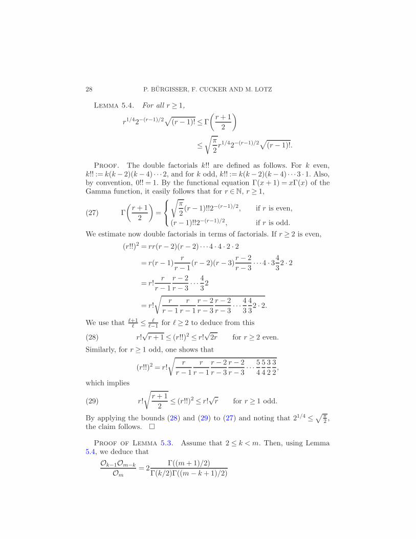
28 P. BURGISSER, F. CUCKER AND M. LOTZ
Lemma 5.4. For all r≥ 1,
r1/42−(r−1)/2√
(r− 1)!≤ Γ
(
r+ 1
2
)
≤√
π
2r1/42−(r−1)/2
√
(r− 1)!.
Proof. The double factorials k!! are defined as follows. For k even,k!! := k(k− 2)(k− 4) · · ·2, and for k odd, k!! := k(k− 2)(k− 4) · · ·3 · 1. Also,by convention, 0!! = 1. By the functional equation Γ(x+ 1) = xΓ(x) of theGamma function, it easily follows that for r ∈N, r ≥ 1,
Γ
(
r+1
2
)
=
√
π
2(r− 1)!!2−(r−1)/2, if r is even,
(r− 1)!!2−(r−1)/2, if r is odd.
(27)
We estimate now double factorials in terms of factorials. If r≥ 2 is even,
(r!!)2 = rr(r− 2)(r − 2) · · ·4 · 4 · 2 · 2
= r(r− 1)r
r− 1(r− 2)(r− 3)
r− 2
r− 3· · ·4 · 34
32 · 2
= r!r
r− 1
r− 2
r− 3· · · 4
32
= r!
√
r
r− 1
r
r− 1
r− 2
r− 3
r− 2
r− 3· · · 4
3
4
32 · 2.
We use that ℓ+1ℓ ≤ ℓ
ℓ−1 for ℓ≥ 2 to deduce from this
r!√r+1≤ (r!!)2 ≤ r!
√2r for r ≥ 2 even.(28)
Similarly, for r≥ 1 odd, one shows that
(r!!)2 = r!
√
r
r− 1
r
r− 1
r− 2
r− 3
r− 2
r− 3· · · 5
4
5
4
3
2
3
2,
which implies
r!
√
r+ 1
2≤ (r!!)2 ≤ r!
√r for r ≥ 1 odd.(29)
By applying the bounds (28) and (29) to (27) and noting that 21/4 ≤√
π2 ,
the claim follows. �
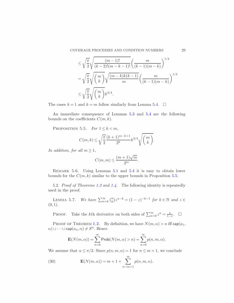
Proof of Lemma 5.3. Assume that 2 ≤ k < m. Then, using Lemma5.4, we deduce that
Ok−1Om−k
Om= 2
Γ((m+ 1)/2)
Γ(k/2)Γ((m− k+1)/2)
COVERAGE PROCESSES AND CONDITION NUMBERS 29
≤√
π
2
√
(m− 1)!
(k− 2)!(m− k− 1)!
(
m
(k− 1)(m− k)
)1/4
=
√
π
2
√
(
mk
)
√
(m− k)k(k − 1)
m
(
m
(k− 1)(m− k)
)1/4
≤√
π
2
√
(
mk
)
k3/4.
The cases k = 1 and k =m follow similarly from Lemma 5.4. �
An immediate consequence of Lemmas 5.3 and 5.4 are the followingbounds on the coefficients C(m,k).
Proposition 5.5. For 1≤ k <m,
C(m,k)≤√
π
2
(k+ 1)m−k+1
2kk3/4
√
(
mk
)
.
In addition, for all m≥ 1,
C(m,m)≤ (m+ 1)√m
2m.
Remark 5.6. Using Lemmas 5.1 and 5.4 it is easy to obtain lowerbounds for the C(m,k) similar to the upper bounds in Proposition 5.5.
5.2. Proof of Theorems 1.2 and 1.4. The following identity is repeatedlyused in the proof.
Lemma 5.7. We have∑∞
n=k
(nk
)
zn−k = (1 − z)−k−1 for k ∈ N and z ∈(0,1).
Proof. Take the kth derivative on both sides of∑∞
n=0 zn = 1
1−z . �
Proof of Theorem 1.2. By definition, we have N(m,α)> n iff cap(a1,α) ∪ · · · ∪ cap(an, α) 6= Sn. Hence
E(N(m,α)) =
∞∑
n=0
Prob(N(m,α)> n) =
∞∑
n=0
p(n,m,α).
We assume that α≤ π/2. Since p(n,m,α) = 1 for n≤m+ 1, we conclude
E(N(m,α)) =m+1+∞∑
n=m+1
p(n,m,α).(30)
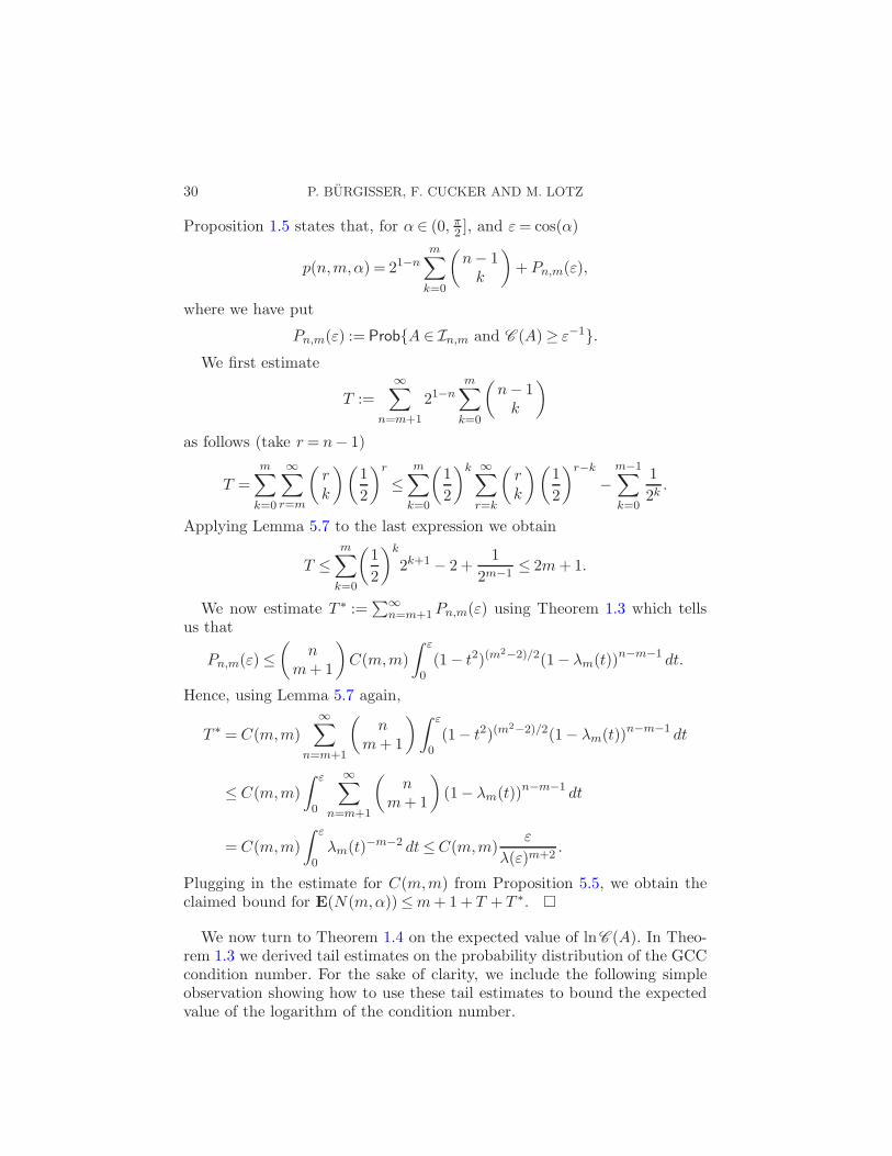
30 P. BURGISSER, F. CUCKER AND M. LOTZ
Proposition 1.5 states that, for α ∈ (0, π2 ], and ε= cos(α)
p(n,m,α) = 21−nm∑
k=0
(
n− 1k
)
+Pn,m(ε),
where we have put
Pn,m(ε) := Prob{A ∈ In,m and C (A)≥ ε−1}.We first estimate
T :=
∞∑
n=m+1
21−nm∑
k=0
(
n− 1k
)
as follows (take r= n− 1)
T =m∑
k=0
∞∑
r=m
(
rk
)(
1
2
)r
≤m∑
k=0
(
1
2
)k ∞∑
r=k
(
rk
)(
1
2
)r−k
−m−1∑
k=0
1
2k.
Applying Lemma 5.7 to the last expression we obtain
T ≤m∑
k=0
(
1
2
)k
2k+1 − 2 +1
2m−1≤ 2m+1.
We now estimate T ∗ :=∑∞
n=m+1Pn,m(ε) using Theorem 1.3 which tellsus that
Pn,m(ε)≤(
nm+ 1
)
C(m,m)
∫ ε
0(1− t2)(m
2−2)/2(1− λm(t))n−m−1 dt.
Hence, using Lemma 5.7 again,
T ∗ = C(m,m)
∞∑
n=m+1
(
nm+1
)∫ ε
0(1− t2)(m
2−2)/2(1− λm(t))n−m−1 dt
≤ C(m,m)
∫ ε
0
∞∑
n=m+1
(
nm+ 1
)
(1− λm(t))n−m−1 dt
= C(m,m)
∫ ε
0λm(t)−m−2 dt≤C(m,m)
ε
λ(ε)m+2.
Plugging in the estimate for C(m,m) from Proposition 5.5, we obtain theclaimed bound for E(N(m,α))≤m+ 1+ T + T ∗. �
We now turn to Theorem 1.4 on the expected value of lnC (A). In Theo-rem 1.3 we derived tail estimates on the probability distribution of the GCCcondition number. For the sake of clarity, we include the following simpleobservation showing how to use these tail estimates to bound the expectedvalue of the logarithm of the condition number.
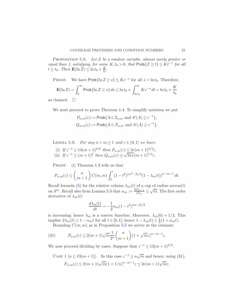
COVERAGE PROCESSES AND CONDITION NUMBERS 31
Proposition 5.8. Let Z be a random variable, almost surely greater orequal than 1, satisfying, for some K, t0 > 0, that Prob{Z ≥ t} ≤Kt−1 for allt≥ t0. Then E(lnZ)≤ ln t0 +
Kt0.
Proof. We have Prob{lnZ ≥ s} ≤Ke−s for all s > ln t0. Therefore,
E(lnZ) =
∫ ∞
0Prob{lnZ ≥ s}ds≤ ln t0 +
∫ ∞
ln t0
Ke−s dt= ln t0 +K
t0
as claimed. �
We next proceed to prove Theorem 1.4. To simplify notation we put
Pn,m(ε) := Prob{A ∈ In,m and C (A)≥ ε−1},Qn,m(ε) := Prob{A ∈Fn,m and C (A)≥ ε−1}.
Lemma 5.9. For any n>m≥ 1 and ε ∈ (0,1] we have:
(i) If ε−1 ≥ 13(m+1)3/2 then Pn,m(ε)≤ 2e(m+1)3/2ε.
(ii) If ε−1 ≥ (m+1)2 then Qn,m(ε)≤√2πe(m+1)7/4ε.
Proof. (i) Theorem 1.3 tells us that
Pn,m(ε)≤(
nm+ 1
)
C(m,m)
∫ ε
0(1− t2)(m
2−2)/2(1− λm(t))n−m−1 dt.
Recall formula (5) for the relative volume λm(t) of a cap of radius arccos(t)
on Sm. Recall also from Lemma 5.3 that αm := 2Om−1
Om≤√
m. The first orderderivative of λm(t)
dλm(t)
dt=−1
2αm(1− t2)(m−2)/2
is increasing; hence λm is a convex function. Moreover, λm(0) = 1/2. Thisimplies 2λm(t)≥ 1−αmt for all t ∈ [0,1]; hence 1− λm(t)≤ 1
2(1 +αmt).Bounding C(m,m) as in Proposition 5.5 we arrive at the estimate
Pn,m(ε)≤ 2(m+1)√m
1
2n
(
n
m+1
)
(1 +√mε)n−m−1ε.(31)
We now proceed dividing by cases. Suppose that ε−1 ≥ 13(m+1)3/2.
Case 1 [n≤ 13(m+1)]. In this case ε−1 ≥ n√m and hence, using (31),
Pn,m(ε)≤ 2(m+1)√m(1 + 1/n)n−m−1ε≤ 2e(m+ 1)
√mε.
32 P. BURGISSER, F. CUCKER AND M. LOTZ
Case 2 [n > 13(m+1)]. This implies ln(e nm+1 )≤ n
m+1 ln(43 ), and it fol-
lows that(
nm+1
)
≤ 1
(m+1)!nm+1 ≤
(
en
m+1
)m+1
≤(
4
3
)n
.(32)
Since, in addition, ε−1 ≥ 13(m+1)√m≥ 2
√m we get from (31)
Pn,m(ε)≤ 2(m+ 1)√m
1
2n
(
nm+1
)(
3
2
)n
ε≤ 2(m+ 1)√mε.
(ii) Theorem 1.3 implies that
Qn,m(ε) =
m∑
k=1
(
nk+ 1
)
C(m,k)
∫ ε
0tm−k(1− t2)km/2−1λm(t)n−k−1 dt
≤m∑
k=1
(
nk+ 1
)
C(m,k)εm−k+12−(n−k−1)
≤m∑
k=1
C(m,k)εm−k+12k+1,
the second line since λm(t)≤ 12 . Using Proposition 5.5 we obtain
Qn,m(ε)≤ ε√2π(m+ 1)7/4
m∑
k=1
√
(
mk
)
((m+ 1)ε)m−k
≤ ε√2π(m+ 1)7/4
m∑
k=1
(
mk
)
((m+1)ε)m−k
≤ ε√2π(m+ 1)7/4(1 + (m+ 1)ε)m.
Under the assumption ε−1 ≥ (m+1)2 we have (m+1)ε≤ 1(m+1) , and hence
Qn,m(ε)≤ ε√2π(m+ 1)7/4
√e. �
Proof of Theorem 1.4. For ε−1 ≥ 13(m + 1)2 we have, by Lemma5.9,
Prob{C (A)≥ ε−1}= Pn,m(ε) +Qn,m(ε)
≤ (2e(m+ 1)3/2 +√2πe(m+ 1)7/4)ε
≤ 9.6(m+ 1)2ε.
An application of Proposition 5.8 with K = 9.6(m+1)2 and t0 = 13(m+1)2
shows that
E(lnC (A))≤ 2 ln(m+ 1) + ln13 + 9.6/13≤ 2 ln(m+1) + 3.31. �
COVERAGE PROCESSES AND CONDITION NUMBERS 33
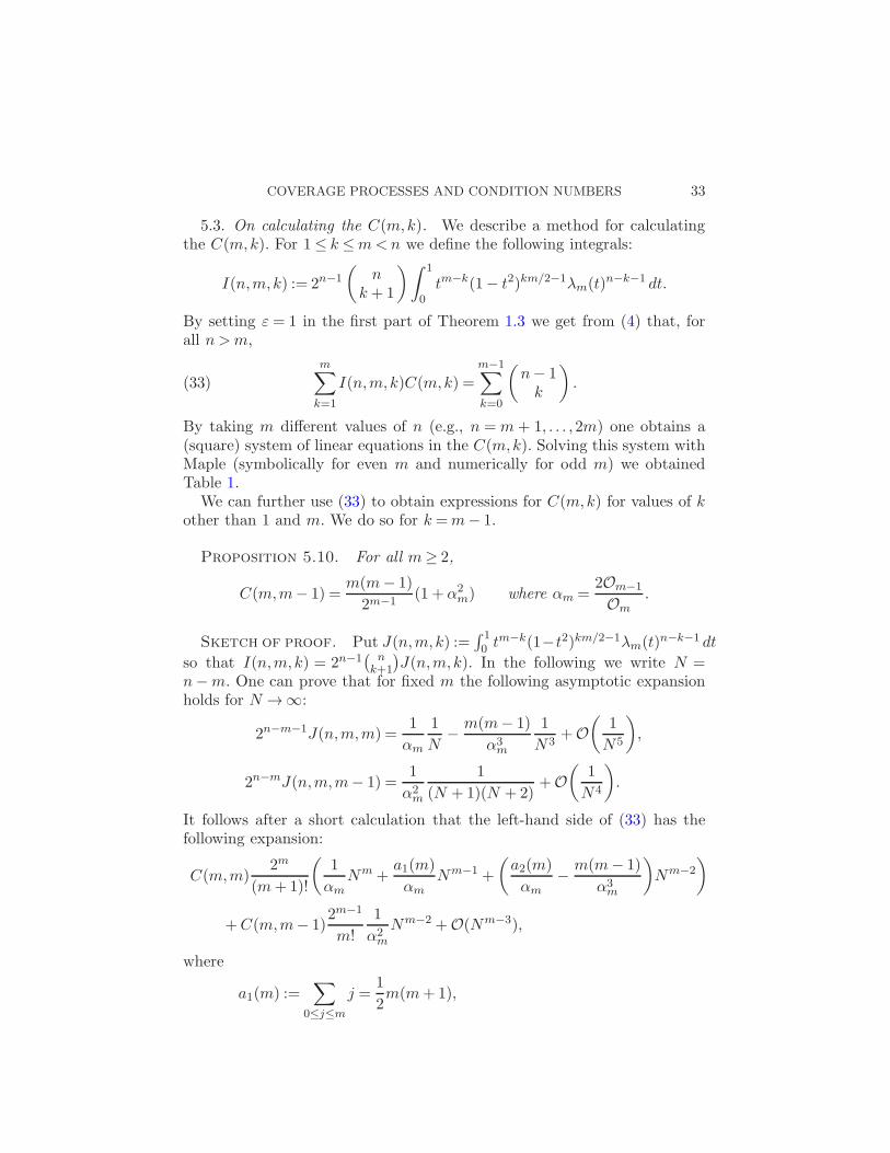
5.3. On calculating the C(m,k). We describe a method for calculatingthe C(m,k). For 1≤ k ≤m<n we define the following integrals:
I(n,m,k) := 2n−1
(
nk+ 1
)∫ 1
0tm−k(1− t2)km/2−1λm(t)n−k−1 dt.
By setting ε= 1 in the first part of Theorem 1.3 we get from (4) that, forall n >m,
m∑
k=1
I(n,m,k)C(m,k) =
m−1∑
k=0
(
n− 1k
)
.(33)
By taking m different values of n (e.g., n =m+ 1, . . . ,2m) one obtains a(square) system of linear equations in the C(m,k). Solving this system withMaple (symbolically for even m and numerically for odd m) we obtainedTable 1.
We can further use (33) to obtain expressions for C(m,k) for values of kother than 1 and m. We do so for k =m− 1.
Proposition 5.10. For all m≥ 2,
C(m,m− 1) =m(m− 1)
2m−1(1 +α2
m) where αm =2Om−1
Om.
Sketch of proof. Put J(n,m,k) :=∫ 10 t
m−k(1−t2)km/2−1λm(t)n−k−1 dt
so that I(n,m,k) = 2n−1( nk+1
)
J(n,m,k). In the following we write N =n−m. One can prove that for fixed m the following asymptotic expansionholds for N →∞:
2n−m−1J(n,m,m) =1
αm
1
N− m(m− 1)
α3m
1
N3+O
(
1
N5
)
,
2n−mJ(n,m,m− 1) =1
α2m
1
(N +1)(N +2)+O
(
1
N4
)
.
It follows after a short calculation that the left-hand side of (33) has thefollowing expansion:
C(m,m)2m
(m+1)!
(
1
αmNm +
a1(m)
αmNm−1 +
(
a2(m)
αm− m(m− 1)
α3m
)
Nm−2
)
+C(m,m− 1)2m−1
m!
1
α2m
Nm−2 +O(Nm−3),
where
a1(m) :=∑
0≤j≤m
j =1
2m(m+1),
34 P. BURGISSER, F. CUCKER AND M. LOTZ
a2(m) :=∑
0≤i<j≤m
ij =1
24(m+1)m(m− 1)(m− 2)(3m+2).
Now we expand the right-hand side of (33) to obtain
1
m!Nm +
(
a1(m− 1)
m!+
1
(m− 1)!
)
Nm−1
+
(
a2(m− 1)
m!+a1(m− 1)
(m− 1)!+
1
(m− 2)!
)
Nm−2
+O(Nm−3).
By comparing the coefficients of Nm (or those of Nm−1) we obtain
C(m,m) =m+1
2mαm.
By comparing the coefficients of Nm−2 we get, after a short calculation,
C(m,m− 1) =O2
m−1
O2m2m−3
(
a2(m− 1)− a2(m) +ma1(m− 1)
+m(m− 1) +m(m− 1)O2
m
4O2m−1
)
,
and simplifying this expression, the claimed result follows. �
Finding a closed form for all coefficients C(m,k) remains a challengingtask.
Acknowledgment. We thank Dennis Amelunxen for pointing out an errorin a previous version in the paper.
REFERENCES
[1] Agmon, S. (1954). The relaxation method for linear inequalities. Canad. J. Math. 6382–392. MR0062786
[2] Burgisser, P. and Amelunxen, D. (2008). Uniform smoothed analysis of a condi-tion number for linear programming. Accepted for Math. Program. A. Availableat arXiv:0803.0925.
[3] Cheung, D. and Cucker, F. (2001). A new condition number for linear program-ming. Math. Program. 91 163–174. MR1865268
[4] Cheung, D. and Cucker, F. (2002). Probabilistic analysis of condition numbers forlinear programming. J. Optim. Theory Appl. 114 55–67. MR1910854
[5] Cheung, D., Cucker, F. and Hauser, R. (2005). Tail decay and moment estimatesof a condition number for random linear conic systems. SIAM J. Optim. 15 1237–1261. MR2178497
COVERAGE PROCESSES AND CONDITION NUMBERS 35
[6] Cucker, F. and Pena, J. (2002). A primal-dual algorithm for solving polyhedralconic systems with a finite-precision machine. SIAM J. Optim. 12 522–554.MR1885574
[7] Cucker, F. and Wschebor, M. (2002). On the expected condition number of linearprogramming problems. Numer. Math. 94 419–478. MR1981163
[8] Dunagan, J., Spielman, D. A. and Teng, S.-H. (2009). Smoothed analysis ofcondition numbers and complexity implications for linear programming. Math.Programming. To appear. Available at http://arxiv.org/abs/cs/0302011v2.
[9] Dvoretzky, A. (1956). On covering a circle by randomly placed arcs. Proc. Natl.Acad. Sci. USA 42 199–203. MR0079365
[10] Gilbert, E. N. (1965). The probability of covering a sphere with N circular caps.Biometrika 52 323–330. MR0207005
[11] Goffin, J.-L. (1980). The relaxation method for solving systems of linear inequali-ties. Math. Oper. Res. 5 388–414. MR594854
[12] Hall, P. (1985). On the coverage of k-dimensional space by k-dimensional spheres.Ann. Probab. 13 991–1002. MR799434
[13] Hall, P. (1988). Introduction to the Theory of Coverage Processes. Wiley, New York.MR973404
[14] Hauser, R. and Muller, T. (2009). Conditioning of random conic systems un-der a general family of input distributions. Found. Comput. Math. 9 335–358.MR2496555
[15] Janson, S. (1986). Random coverings in several dimensions. Acta Math. 156 83–118.MR822331
[16] Kahane, J.-P. (1959). Sur le recouvrement d’un cercle par des arcs disposes auhasard. C. R. Math. Acad. Sci. Paris 248 184–186. MR0103533
[17] Miles, R. E. (1968). Random caps on a sphere. Ann. Math. Statist. 39 1371.[18] Miles, R. E. (1969). The asymptotic values of certain coverage probabilities.
Biometrika 56 661–680. MR0254953[19] Miles, R. E. (1971). Isotropic random simplices. Adv. in Appl. Probab. 3 353–382.
MR0309164[20] Moran, P. A. P. and Fazekas de St. Groth, S. (1962). Random circles on a
sphere. Biometrika 49 389–396. MR0156434[21] Motzkin, T. S. and Schoenberg, I. J. (1954). The relaxation method for linear
inequalities. Canad. J. Math. 6 393–404. MR0062787[22] Reitzner, M. (2002). Random points on the boundary of smooth convex bodies.
Trans. Amer. Math. Soc. 354 2243–2278. MR1885651[23] Rosenblatt, F. (1962). Principles of Neurodynamics. Perceptrons and the Theory
of Brain Mechanisms. Spartan Books, Washington, DC. MR0135635[24] Santalo, L. A. (1976). Integral Geometry and Geometric Probability. Addison-
Wesley, Reading, MA. MR0433364[25] Siegel, A. F. (1979). Asymptotic coverage distributions on the circle. Ann. Probab.
7 651–661. MR537212[26] Siegel, A. F. and Holst, L. (1982). Covering the circle with random arcs of random
sizes. J. Appl. Probab. 19 373–381. MR649974[27] Solomon, H. (1978). Geometric Probability. SIAM, Philadelphia, PA. MR0488215[28] Stevens, W. L. (1939). Solution to a geometrical problem in probability. Ann.
Eugenics 9 315–320. MR0001479[29] Wendel, J. G. (1962). A problem in geometric probability.Math. Scand. 11 109–111.
MR0146858[30] Whitworth, W. A. (1965). DCC Exercises in Choice and Chance. Dover, New York.
36 P. BURGISSER, F. CUCKER AND M. LOTZ
[31] Zahle, M. (1990). A kinematic formula and moment measures of random sets. Math.Nachr. 149 325–340. MR1124814
P. Burgisser
Institute of Mathematics
University of Paderborn
33098 Paderborn
Germany
E-mail: [email protected]
F. Cucker
Department of Mathematics
City University of Hong Kong
Kowloon Tong
Hong Kong
E-mail: [email protected]
M. Lotz
Mathematical Institute
University of Oxford
24-29 St. Giles’
Oxford OX1 3LB
England
E-mail: [email protected]