Course Notes on Computational Financeseydel/cfcoursenotes4beam.pdf · Seydel: Course Notes on...
57
Course Notes on Computational Finance 4 Finite-Difference Methods for American Vanilla Options
Transcript of Course Notes on Computational Financeseydel/cfcoursenotes4beam.pdf · Seydel: Course Notes on...
Seydel: Course Notes on Computational Finan e, Chapter 4 (Version 2015) 400
Course Notes on
Computational Finance
4Finite-Difference Methods
for American Vanilla Options
Seydel: Course Notes on Computational Finan e, Chapter 4 (Version 2015) 401
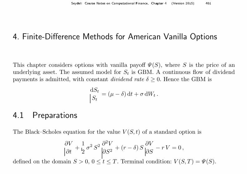
4. Finite-Difference Methods for American Vanilla Options
This chapter considers options with vanilla payoff Ψ(S), where S is the price of anunderlying asset. The assumed model for St is GBM. A continuous flow of dividendpayments is admitted, with constant dividend rate δ ≥ 0. Hence the GBM is
dSt
St
= (µ − δ) dt + σ dWt .
4.1 Preparations
The Black–Scholes equation for the value V (S, t) of a standard option is
∂V
∂t+
1
2σ2 S2 ∂2V
∂S2+ (r − δ)S
∂V
∂S− r V = 0 ,
defined on the domain S > 0, 0 ≤ t ≤ T . Terminal condition: V (S, T ) = Ψ(S).
Seydel: Course Notes on Computational Finan e, Chapter 4 (Version 2015) 402
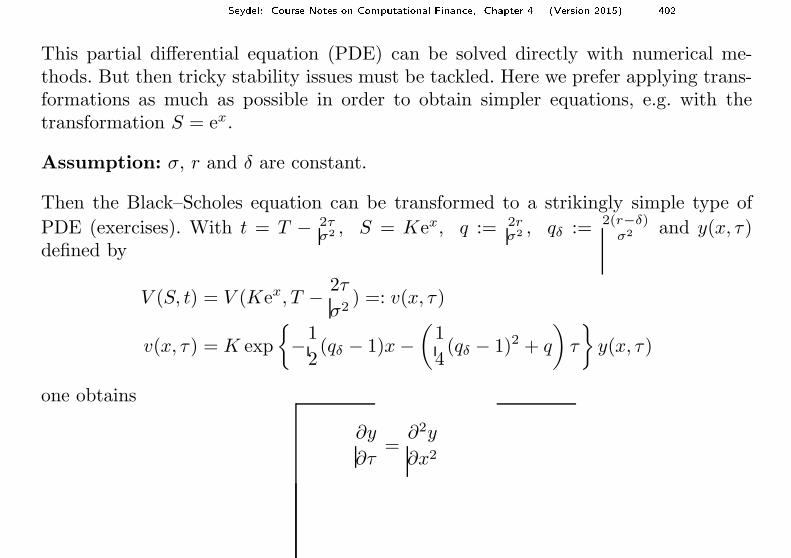
This partial differential equation (PDE) can be solved directly with numerical me-thods. But then tricky stability issues must be tackled. Here we prefer applying trans-formations as much as possible in order to obtain simpler equations, e.g. with thetransformation S = ex.
Assumption: σ, r and δ are constant.
Then the Black–Scholes equation can be transformed to a strikingly simple type of
PDE (exercises). With t = T − 2τσ2 , S = Kex, q := 2r
σ2 , qδ := 2(r−δ)σ2 and y(x, τ)
defined by
V (S, t) = V (Kex, T − 2τ
σ2) =: v(x, τ)
v(x, τ) = K exp
{
−1
2(qδ − 1)x −
(1
4(qδ − 1)2 + q
)
τ
}
y(x, τ)
one obtains
∂y
∂τ=
∂2y
∂x2
Seydel: Course Notes on Computational Finan e, Chapter 4 (Version 2015) 403
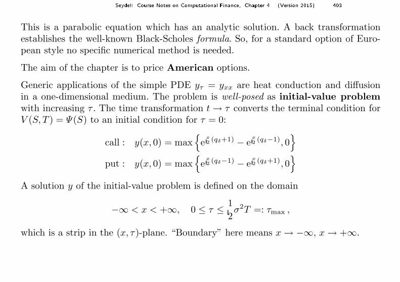
This is a parabolic equation which has an analytic solution. A back transformationestablishes the well-known Black-Scholes formula. So, for a standard option of Euro-pean style no specific numerical method is needed.
The aim of the chapter is to price American options.
Generic applications of the simple PDE yτ = yxx are heat conduction and diffusionin a one-dimensional medium. The problem is well-posed as initial-value problemwith increasing τ . The time transformation t → τ converts the terminal condition forV (S, T ) = Ψ(S) to an initial condition for τ = 0:
call : y(x, 0) = max{
ex2(qδ+1) − e
x2(qδ−1), 0
}
put : y(x, 0) = max{
ex2(qδ−1) − e
x2(qδ+1), 0
}
A solution y of the initial-value problem is defined on the domain
−∞ < x < +∞, 0 ≤ τ ≤ 1
2σ2T =: τmax ,
which is a strip in the (x, τ)-plane. “Boundary” here means x → −∞, x → +∞.
Seydel: Course Notes on Computational Finan e, Chapter 4 (Version 2015) 404
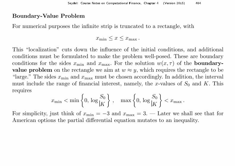
Boundary-Value Problem
For numerical purposes the infinite strip is truncated to a rectangle, with
xmin ≤ x ≤ xmax .
This “localization” cuts down the influence of the initial conditions, and additionalconditions must be formulated to make the problem well-posed. These are boundaryconditions for the sides xmin and xmax. For the solution w(x, τ) of the boundary-value problem on the rectangle we aim at w ≈ y, which requires the rectangle to be“large.” The sides xmin and xmax must be chosen accordingly. In addition, the intervalmust include the range of financial interest, namely, the x-values of S0 and K. Thisrequires
xmin < min
{
0, logS0
K
}
, max
{
0, logS0
K
}
< xmax .
For simplicity, just think of xmin = −3 and xmax = 3. — Later we shall see that forAmerican options the partial differential equation mutates to an inequality.
Seydel: Course Notes on Computational Finan e, Chapter 4 (Version 2015) 405
4.2 Basics of Finite-Difference Methods (FDM)
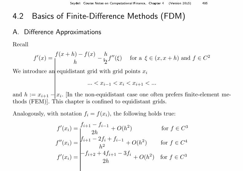
A. Difference Approximations
Recall
f ′(x) =f(x + h) − f(x)
h− h
2f ′′(ξ) for a ξ ∈ (x, x + h) and f ∈ C2
We introduce an equidistant grid with grid points xi
... < xi−1 < xi < xi+1 < ...
and h := xi+1 − xi. [In the non-equidistant case one often prefers finite-element me-thods (FEM)]. This chapter is confined to equidistant grids.
Analogously, with notation fi = f(xi), the following holds true:
f ′(xi) =fi+1 − fi−1
2h+ O(h2) for f ∈ C3
f ′′(xi) =fi+1 − 2fi + fi−1
h2+ O(h2) for f ∈ C4
f ′(xi) =−fi+2 + 4fi+1 − 3fi
2h+ O(h2) for f ∈ C3
Seydel: Course Notes on Computational Finan e, Chapter 4 (Version 2015) 406
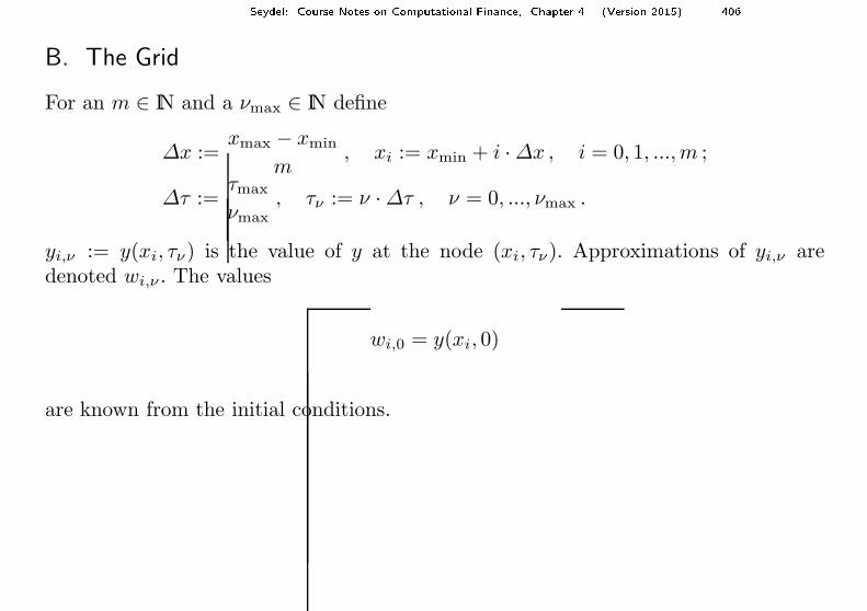
B. The Grid
For an m ∈ IN and a νmax ∈ IN define
∆x :=xmax − xmin
m, xi := xmin + i · ∆x , i = 0, 1, ...,m ;
∆τ :=τmax
νmax, τν := ν · ∆τ , ν = 0, ..., νmax .
yi,ν := y(xi, τν) is the value of y at the node (xi, τν). Approximations of yi,ν aredenoted wi,ν . The values
wi,0 = y(xi, 0)
are known from the initial conditions.
Seydel: Course Notes on Computational Finan e, Chapter 4 (Version 2015) 407
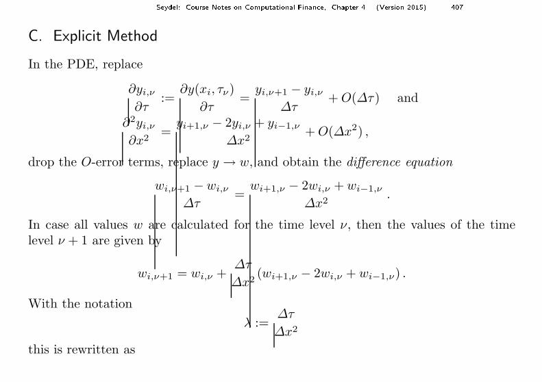
C. Explicit Method
In the PDE, replace
∂yi,ν
∂τ:=
∂y(xi, τν)
∂τ=
yi,ν+1 − yi,ν
∆τ+ O(∆τ) and
∂2yi,ν
∂x2=
yi+1,ν − 2yi,ν + yi−1,ν
∆x2+ O(∆x2) ,
drop the O-error terms, replace y → w, and obtain the difference equation
wi,ν+1 − wi,ν
∆τ=
wi+1,ν − 2wi,ν + wi−1,ν
∆x2.
In case all values w are calculated for the time level ν, then the values of the timelevel ν + 1 are given by
wi,ν+1 = wi,ν +∆τ
∆x2(wi+1,ν − 2wi,ν + wi−1,ν) .
With the notation
λ :=∆τ
∆x2
this is rewritten as
Seydel: Course Notes on Computational Finan e, Chapter 4 (Version 2015) 408
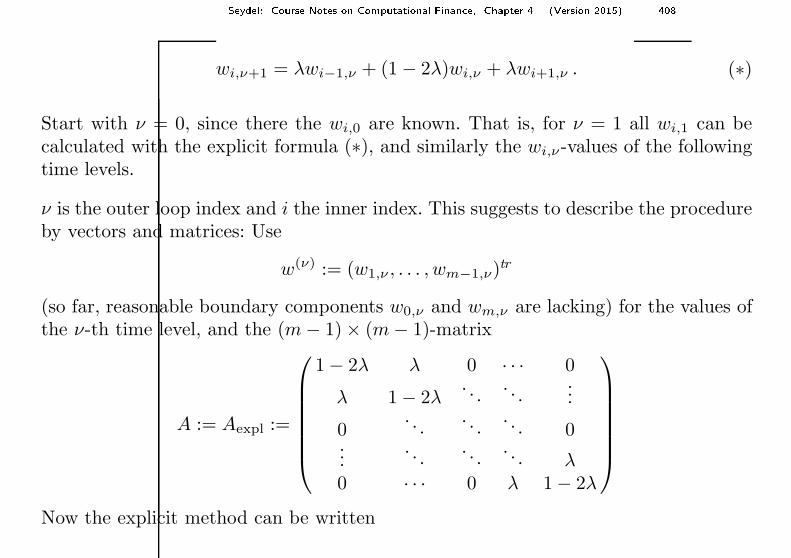
wi,ν+1 = λwi−1,ν + (1 − 2λ)wi,ν + λwi+1,ν . (∗)
Start with ν = 0, since there the wi,0 are known. That is, for ν = 1 all wi,1 can becalculated with the explicit formula (∗), and similarly the wi,ν -values of the followingtime levels.
ν is the outer loop index and i the inner index. This suggests to describe the procedureby vectors and matrices: Use
w(ν) := (w1,ν , . . . , wm−1,ν)tr
(so far, reasonable boundary components w0,ν and wm,ν are lacking) for the values ofthe ν-th time level, and the (m − 1) × (m − 1)-matrix
A := Aexpl :=
1 − 2λ λ 0 · · · 0
λ 1 − 2λ. . .
. . ....
0. . .
. . .. . . 0
.... . .
. . .. . . λ
0 · · · 0 λ 1 − 2λ
Now the explicit method can be written
Seydel: Course Notes on Computational Finan e, Chapter 4 (Version 2015) 409
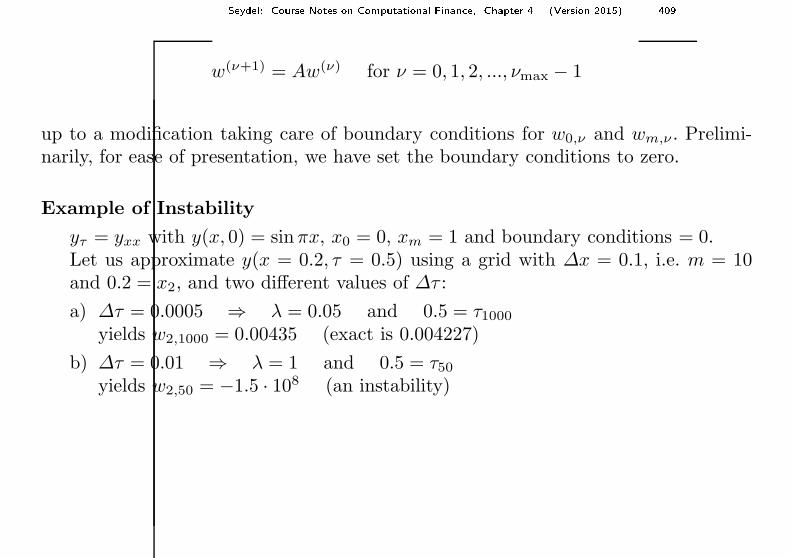
w(ν+1) = Aw(ν) for ν = 0, 1, 2, ..., νmax − 1
up to a modification taking care of boundary conditions for w0,ν and wm,ν . Prelimi-narily, for ease of presentation, we have set the boundary conditions to zero.
Example of Instability
yτ = yxx with y(x, 0) = sinπx, x0 = 0, xm = 1 and boundary conditions = 0.Let us approximate y(x = 0.2, τ = 0.5) using a grid with ∆x = 0.1, i.e. m = 10and 0.2 = x2, and two different values of ∆τ :
a) ∆τ = 0.0005 ⇒ λ = 0.05 and 0.5 = τ1000
yields w2,1000 = 0.00435 (exact is 0.004227)
b) ∆τ = 0.01 ⇒ λ = 1 and 0.5 = τ50
yields w2,50 = −1.5 · 108 (an instability)
Seydel: Course Notes on Computational Finan e, Chapter 4 (Version 2015) 410
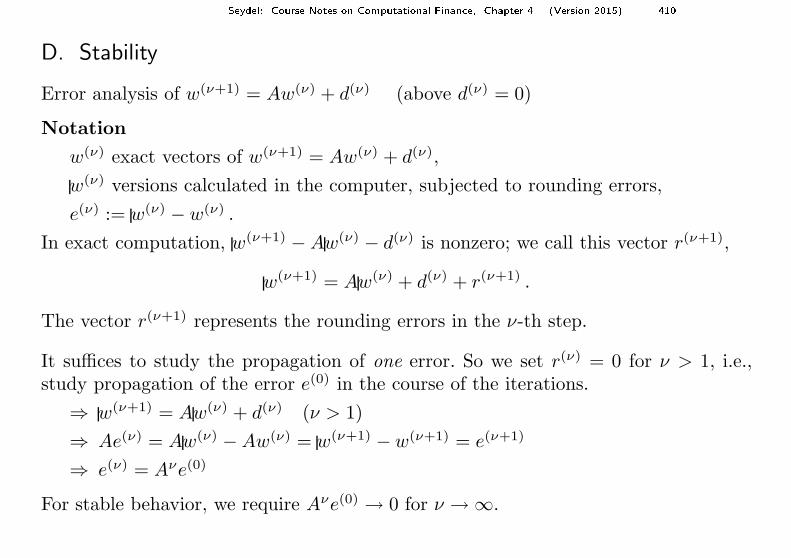
D. Stability
Error analysis of w(ν+1) = Aw(ν) + d(ν) (above d(ν) = 0)
Notation
w(ν) exact vectors of w(ν+1) = Aw(ν) + d(ν),
w(ν) versions calculated in the computer, subjected to rounding errors,
e(ν) := w(ν) − w(ν) .
In exact computation, w(ν+1) − Aw(ν) − d(ν) is nonzero; we call this vector r(ν+1),
w(ν+1) = Aw(ν) + d(ν) + r(ν+1) .
The vector r(ν+1) represents the rounding errors in the ν-th step.
It suffices to study the propagation of one error. So we set r(ν) = 0 for ν > 1, i.e.,study propagation of the error e(0) in the course of the iterations.
⇒ w(ν+1) = Aw(ν) + d(ν) (ν > 1)
⇒ Ae(ν) = Aw(ν) − Aw(ν) = w(ν+1) − w(ν+1) = e(ν+1)
⇒ e(ν) = Aνe(0)
For stable behavior, we require Aνe(0) → 0 for ν → ∞.
Seydel: Course Notes on Computational Finan e, Chapter 4 (Version 2015) 411
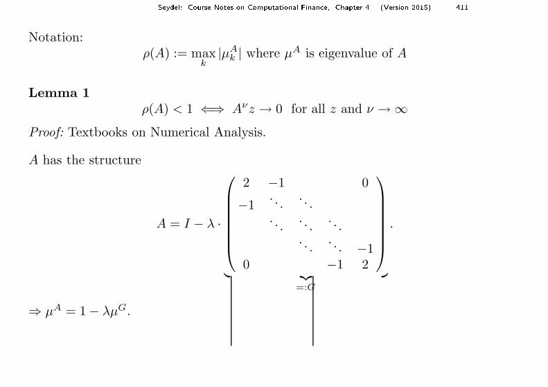
Notation:ρ(A) := max
k|µA
k | where µA is eigenvalue of A
Lemma 1ρ(A) < 1 ⇐⇒ Aνz → 0 for all z and ν → ∞
Proof: Textbooks on Numerical Analysis.
A has the structure
A = I − λ ·
2 −1 0
−1. . .
. . .. . .
. . .. . .
. . .. . . −1
0 −1 2
︸ ︷︷ ︸
=:G
.
⇒ µA = 1 − λµG.
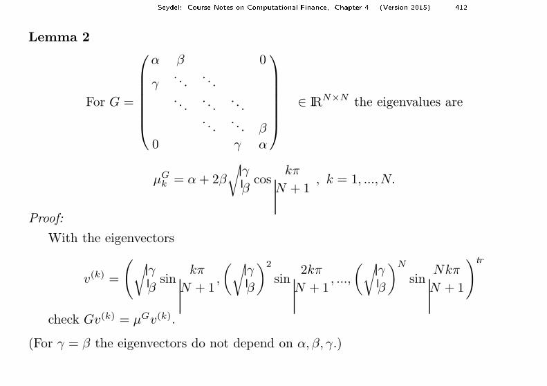
Seydel: Course Notes on Computational Finan e, Chapter 4 (Version 2015) 412
Lemma 2
For G =
α β 0
γ. . .
. . .. . .
. . .. . .
. . .. . . β
0 γ α
∈ IRN×N the eigenvalues are
µGk = α + 2β
√γ
βcos
kπ
N + 1, k = 1, ..., N.
Proof:
With the eigenvectors
v(k) =
(√
γ
βsin
kπ
N + 1,
(√γ
β
)2
sin2kπ
N + 1, ...,
(√γ
β
)N
sinNkπ
N + 1
)tr
check Gv(k) = µGv(k).
(For γ = β the eigenvectors do not depend on α, β, γ.)
Seydel: Course Notes on Computational Finan e, Chapter 4 (Version 2015) 413
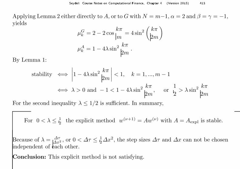
Applying Lemma 2 either directly to A, or to G with N = m−1, α = 2 and β = γ = −1,yields
µGk = 2 − 2 cos
kπ
m= 4 sin2
(kπ
2m
)
µAk = 1 − 4λ sin2 kπ
2m.
By Lemma 1:
stability ⇐⇒∣∣∣∣1 − 4λ sin2 kπ
2m
∣∣∣∣< 1, k = 1, ...,m − 1
⇐⇒ λ > 0 and − 1 < 1 − 4λ sin2 kπ
2m, or
1
2> λ sin2 kπ
2m
For the second inequality λ ≤ 1/2 is sufficient. In summary,
For 0 < λ ≤ 12
the explicit method w(ν+1) = Aw(ν) with A = Aexpl is stable.
Because of λ = ∆τ∆x2 , or 0 < ∆τ ≤ 1
2∆x2, the step sizes ∆τ and ∆x can not be chosenindependent of each other.
Conclusion: This explicit method is not satisfying.
Seydel: Course Notes on Computational Finan e, Chapter 4 (Version 2015) 414
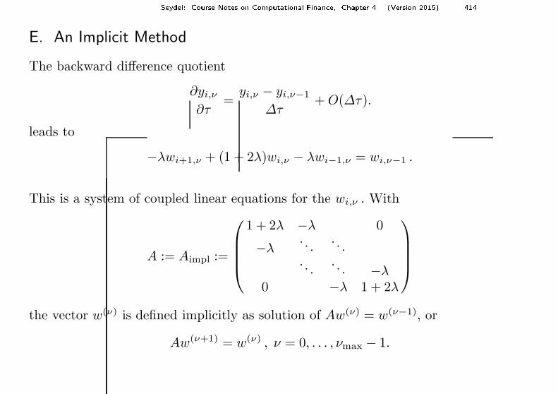
E. An Implicit Method
The backward difference quotient
∂yi,ν
∂τ=
yi,ν − yi,ν−1
∆τ+ O(∆τ).
leads to
−λwi+1,ν + (1 + 2λ)wi,ν − λwi−1,ν = wi,ν−1 .
This is a system of coupled linear equations for the wi,ν . With
A := Aimpl :=
1 + 2λ −λ 0
−λ. . .
. . .. . .
. . . −λ0 −λ 1 + 2λ
the vector w(ν) is defined implicitly as solution of Aw(ν) = w(ν−1), or
Aw(ν+1) = w(ν) , ν = 0, . . . , νmax − 1.
Seydel: Course Notes on Computational Finan e, Chapter 4 (Version 2015) 415
(We still use the preliminary boundary conditions w0,ν = wm,ν = 0.) This methodis called backward difference method or backward time centered space (BTCS) or fullyimplicit.
Stability
The above Lemmas imply that the method is unconditionally stable, and ∆τ and∆x can be chosen independent of each other.
Costs
νmaxO(m), since only one LR-decomposition of A for ν = 0 is necessary (cheap fora tridiagonal matrix). For each ν, only one backward loop is required, which costsO(m) operations.
A weakness of this method (and of the explicit method) is the accuracy of the firstorder in ∆τ , the error is of the order
O(∆x2) + O(∆τ) .
Seydel: Course Notes on Computational Finan e, Chapter 4 (Version 2015) 416
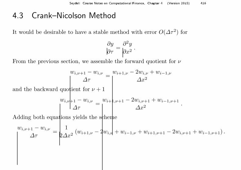
4.3 Crank–Nicolson Method
It would be desirable to have a stable method with error O(∆τ2) for
∂y
∂τ=
∂2y
∂x2.
From the previous section, we assemble the forward quotient for ν
wi,ν+1 − wi,ν
∆τ=
wi+1,ν − 2wi,ν + wi−1,ν
∆x2
and the backward quotient for ν + 1
wi,ν+1 − wi,ν
∆τ=
wi+1,ν+1 − 2wi,ν+1 + wi−1,ν+1
∆x2.
Adding both equations yields the scheme
wi,ν+1 − wi,ν
∆τ=
1
2∆x2(wi+1,ν − 2wi,ν + wi−1,ν + wi+1,ν+1 − 2wi,ν+1 + wi−1,ν+1) .
Seydel: Course Notes on Computational Finan e, Chapter 4 (Version 2015) 417
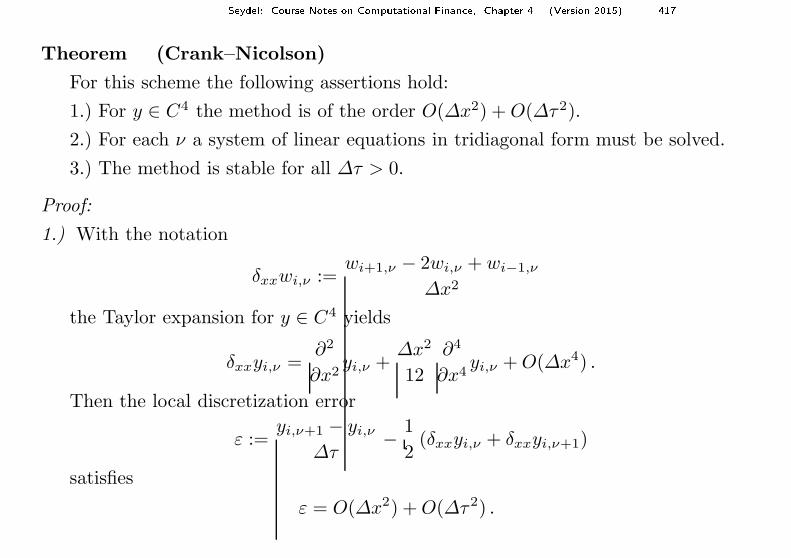
Theorem (Crank–Nicolson)
For this scheme the following assertions hold:
1.) For y ∈ C4 the method is of the order O(∆x2) + O(∆τ2).
2.) For each ν a system of linear equations in tridiagonal form must be solved.
3.) The method is stable for all ∆τ > 0.
Proof:
1.) With the notation
δxxwi,ν :=wi+1,ν − 2wi,ν + wi−1,ν
∆x2
the Taylor expansion for y ∈ C4 yields
δxxyi,ν =∂2
∂x2yi,ν +
∆x2
12
∂4
∂x4yi,ν + O(∆x4) .
Then the local discretization error
ε :=yi,ν+1 − yi,ν
∆τ− 1
2(δxxyi,ν + δxxyi,ν+1)
satisfies
ε = O(∆x2) + O(∆τ2) .
Seydel: Course Notes on Computational Finan e, Chapter 4 (Version 2015) 418
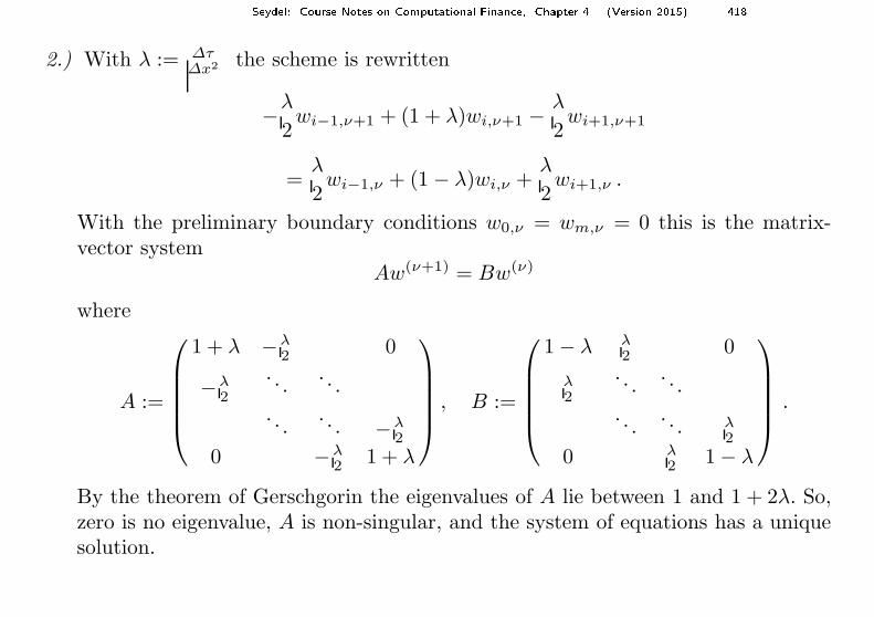
2.) With λ := ∆τ∆x2 the scheme is rewritten
−λ
2wi−1,ν+1 + (1 + λ)wi,ν+1 −
λ
2wi+1,ν+1
=λ
2wi−1,ν + (1 − λ)wi,ν +
λ
2wi+1,ν .
With the preliminary boundary conditions w0,ν = wm,ν = 0 this is the matrix-vector system
Aw(ν+1) = Bw(ν)
where
A :=
1 + λ −λ2 0
−λ2
. . .. . .
. . .. . . −λ
2
0 −λ2 1 + λ
, B :=
1 − λ λ2 0
λ2
. . .. . .
. . .. . . λ
2
0 λ2 1 − λ
.
By the theorem of Gerschgorin the eigenvalues of A lie between 1 and 1 + 2λ. So,zero is no eigenvalue, A is non-singular, and the system of equations has a uniquesolution.
Seydel: Course Notes on Computational Finan e, Chapter 4 (Version 2015) 419
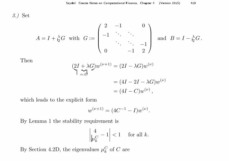
3.) Set
A = I + λ2 G with G :=
2 −1 0
−1. . .
. . .. . .
. . . −10 −1 2
and B = I − λ2 G .
Then(2I + λG︸ ︷︷ ︸
=:C
)w(ν+1) = (2I − λG)w(ν)
= (4I − 2I − λG)w(ν)
= (4I − C)w(ν) ,
which leads to the explicit form
w(ν+1) = (4C−1 − I)w(ν).
By Lemma 1 the stability requirement is∣∣∣∣
4
µCk
− 1
∣∣∣∣< 1 for all k.
By Section 4.2D, the eigenvalues µCk of C are
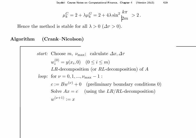
Seydel: Course Notes on Computational Finan e, Chapter 4 (Version 2015) 420
µCk = 2 + λµG
k = 2 + 4λ sin2 kπ
2m> 2 .
Hence the method is stable for all λ > 0 (∆τ > 0).
Algorithm (Crank–Nicolson)
start: Choose m, νmax; calculate ∆x,∆τ
w(0)i = y(xi, 0) (0 ≤ i ≤ m)
LR-decomposition (or RL-decomposition) of A
loop: for ν = 0, 1, ..., νmax − 1 :
c := Bw(ν) + 0 (preliminary boundary conditions 0)
Solve Ax = c (using the LR/RL-decomposition)
w(ν+1) := x
Seydel: Course Notes on Computational Finan e, Chapter 4 (Version 2015) 421
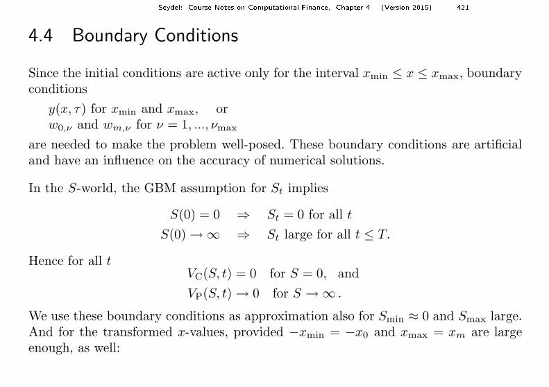
4.4 Boundary Conditions
Since the initial conditions are active only for the interval xmin ≤ x ≤ xmax, boundaryconditions
y(x, τ) for xmin and xmax, orw0,ν and wm,ν for ν = 1, ..., νmax
are needed to make the problem well-posed. These boundary conditions are artificialand have an influence on the accuracy of numerical solutions.
In the S-world, the GBM assumption for St implies
S(0) = 0 ⇒ St = 0 for all t
S(0) → ∞ ⇒ St large for all t ≤ T.
Hence for all tVC(S, t) = 0 for S = 0, and
VP(S, t) → 0 for S → ∞ .
We use these boundary conditions as approximation also for Smin ≈ 0 and Smax large.And for the transformed x-values, provided −xmin = −x0 and xmax = xm are largeenough, as well:
Seydel: Course Notes on Computational Finan e, Chapter 4 (Version 2015) 422
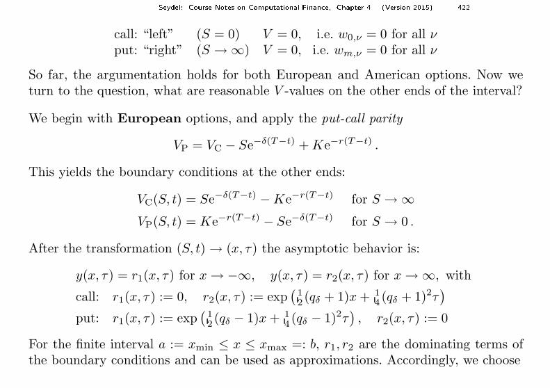
call: “left” (S = 0) V = 0, i.e. w0,ν = 0 for all νput: “right” (S → ∞) V = 0, i.e. wm,ν = 0 for all ν
So far, the argumentation holds for both European and American options. Now weturn to the question, what are reasonable V -values on the other ends of the interval?
We begin with European options, and apply the put-call parity
VP = VC − Se−δ(T−t) + Ke−r(T−t) .
This yields the boundary conditions at the other ends:
VC(S, t) = Se−δ(T−t) − Ke−r(T−t) for S → ∞VP(S, t) = Ke−r(T−t) − Se−δ(T−t) for S → 0 .
After the transformation (S, t) → (x, τ) the asymptotic behavior is:
y(x, τ) = r1(x, τ) for x → −∞, y(x, τ) = r2(x, τ) for x → ∞, with
call: r1(x, τ) := 0, r2(x, τ) := exp(
12 (qδ + 1)x + 1
4 (qδ + 1)2τ)
put: r1(x, τ) := exp(
12 (qδ − 1)x + 1
4 (qδ − 1)2τ), r2(x, τ) := 0
For the finite interval a := xmin ≤ x ≤ xmax =: b, r1, r2 are the dominating terms ofthe boundary conditions and can be used as approximations. Accordingly, we choose
Seydel: Course Notes on Computational Finan e, Chapter 4 (Version 2015) 423
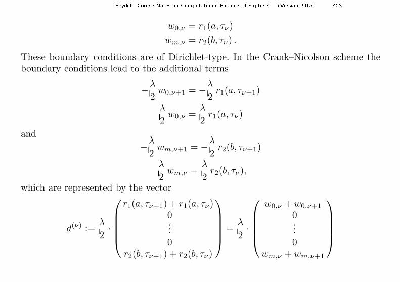
w0,ν = r1(a, τν)
wm,ν = r2(b, τν) .
These boundary conditions are of Dirichlet-type. In the Crank–Nicolson scheme theboundary conditions lead to the additional terms
−λ
2w0,ν+1 = −λ
2r1(a, τν+1)
λ
2w0,ν =
λ
2r1(a, τν)
and
−λ
2wm,ν+1 = −λ
2r2(b, τν+1)
λ
2wm,ν =
λ
2r2(b, τν),
which are represented by the vector
d(ν) :=λ
2·
r1(a, τν+1) + r1(a, τν)0...0
r2(b, τν+1) + r2(b, τν)
=λ
2·
w0,ν + w0,ν+1
0...0
wm,ν + wm,ν+1

Seydel: Course Notes on Computational Finan e, Chapter 4 (Version 2015) 424
In the Crank–Nicolson algorithm the right-hand side of the system of equations is now
c := Bw(ν) + d(ν) ;
the matrix A is unchanged:
Aw(ν) = Bw(ν) + d(ν)
We still need to specify the boundary conditions (b.c.) for American-style optionson the “other” side, namely, left-hand b.c. for the put and right-hand b.c. for the call.
Seydel: Course Notes on Computational Finan e, Chapter 4 (Version 2015) 425
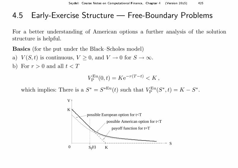
4.5 Early-Exercise Structure — Free-Boundary Problems
For a better understanding of American options a further analysis of the solutionstructure is helpful.
Basics (for the put under the Black–Scholes model)
a) V (S, t) is continuous, V ≥ 0, and V → 0 for S → ∞.
b) For r > 0 and all t < T
V EuP (0, t) = Ke−r(T−t) < K ,
which implies: There is a S∗ = S∗Eu(t) such that V EuP (S∗, t) = K − S∗.
(t)fSS
0
V
possible European option for t<T
possible American option for t<T
payoff function for t=T
K
K
Seydel: Course Notes on Computational Finan e, Chapter 4 (Version 2015) 426
c) VP is monotonic decreasing w.r.t. S, and convex. [R.C.Merton: Theory of RationalOption Pricing (1973)]
Hence S∗ is unique.
d) V AmP ≥ (K − S)+ and V Am
P ≤ K
Assertion 1
Also for the American put with r > 0 there is an S∗ > 0, such that V AmP (S∗, t) =
K − S∗.
Proof:
Assume: V AmP > K − S for all S > 0.
Then−V Am
P + K − S < 0 ,
i.e., exercising the put leads to a loss for all S. Accordingly, early exercise does notmake sense, and hence V Am
P = V EuP . Consequently,
V EuP = V Am
P > K − S ,
for all S > 0, which contradicts the implication of b).
Redefine S∗ := max{S | V Am(S, t) = K − S .}By c) and d), V = K − S for all S < S∗.
Seydel: Course Notes on Computational Finan e, Chapter 4 (Version 2015) 427
It remains to investigate the behavior of V for S ≥ S∗.
Assertion 2
The right-hand side derivative of the function V AmP (S, t) at S∗ has the value −1.
Proof (outline):
We use the notation V := V AmP .
For the right-hand derivative ∂V (S∗,t)∂S
< −1 is impossible, because otherwise for
S > S∗ the property d) is violated. Hence ∂V (S∗,t)∂S
≥ −1.
Assumption:∂V (S∗, t)
∂S> −1 .
We lead this to a contradiction as follows:Build a portfolio: Π := V + S, with initial wealth
Π∗ := V + S∗ .
(= K; borrow from the bank the amount K.) For our GBM
dS = rS dt + σS dW
assume that dt is so small that√
dt ≫ dt. If dt is small enough, then (intuitively)
Seydel: Course Notes on Computational Finan e, Chapter 4 (Version 2015) 428
dW > 0 ⇐⇒ dS > 0 .
The Ito-Lemma leads to
dΠ = (. . .)dt +∂Π
∂SσS dW
= O(dt) +
(∂V
∂S+ 1
)
σS dW.
For dS > 0 this is positive for sufficiently small dt because dW > 0.For dS < 0 the wealth of the portfolio is Π ≡ K and hence dΠ = 0.
In summary: E(dΠ) > 0, and E(dΠ) is of the order O(√
dt). Sell the portfolio afterdt and expect the following balance
Π∗ + E(dΠ) − Kerdt = V + S∗ + E(dΠ) − K(1 + O(dt))
= E(dΠ) + O(dt)
This is positive because E(dΠ) dominates, and we have arrived at a contradictionto the no-arbitrage principle.
Often related proofs use an argument of maximizing the value of the option. In thisway, the perpetual option (an option that does not expire) can be analyzed, see theExercises.
Seydel: Course Notes on Computational Finan e, Chapter 4 (Version 2015) 429
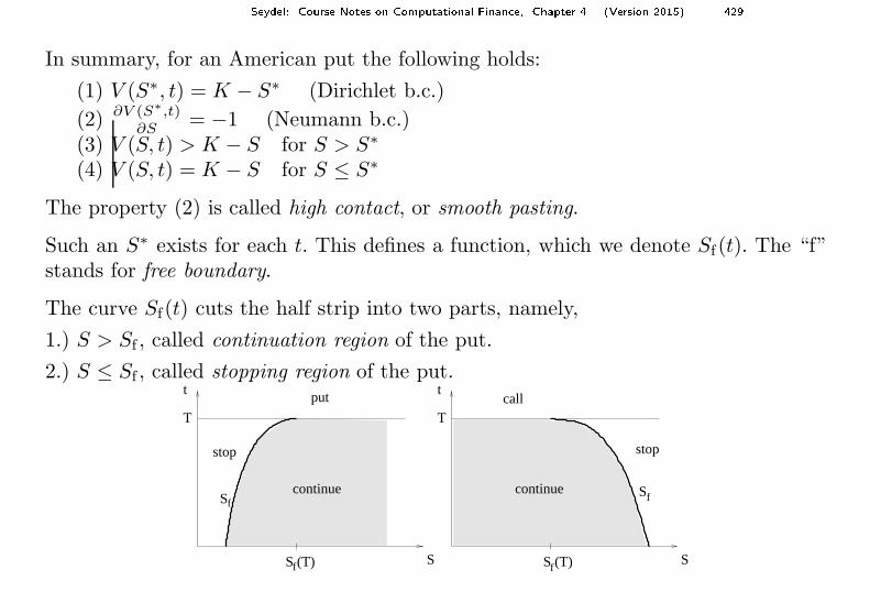
In summary, for an American put the following holds:
(1) V (S∗, t) = K − S∗ (Dirichlet b.c.)
(2) ∂V (S∗,t)∂S
= −1 (Neumann b.c.)(3) V (S, t) > K − S for S > S∗
(4) V (S, t) = K − S for S ≤ S∗
The property (2) is called high contact, or smooth pasting.
Such an S∗ exists for each t. This defines a function, which we denote Sf(t). The “f”stands for free boundary.
The curve Sf(t) cuts the half strip into two parts, namely,
1.) S > Sf , called continuation region of the put.
2.) S ≤ Sf , called stopping region of the put.
continuecontinue
T
S
stop
t
T
S
call
stop
t
S (T) S (T)
put
S
f f
fS f
Seydel: Course Notes on Computational Finan e, Chapter 4 (Version 2015) 430
For standard options without dividend payments, these domains are simply connected.The curve Sf(t) is the interface.
Early-Exercise Curve
The curve Sf(t) is the early-exercise curve by the following reasons:
1.) In case VP > (K − S)+, exercising amounts to −V + K − S < 0. This is a loss.Consequently, the holder continues to hold the option.
2.) In case the price S passes the curve, S < Sf(t), then immediate exercising makessense (“stopping”), because the amount K can be invested, leading for r > 0, t < Tto the profit:
Ker(T−t) − K = K(er(T−t) − 1).
By exercising, the final balance Ker(T−t) is larger than Seδ(T−t), at least for r(T −t) < 1.
Seydel: Course Notes on Computational Finan e, Chapter 4 (Version 2015) 431
Free-Boundary Problem means:
The Black–Scholes equation is valid only in the continuation region, not in thestopping region. Hence the domain for the BS equation for an American-style putis
Sf(t) < S < ∞ .
The left-hand boundary Sf(t) is “free” in the sense that it is unknown initially. Itis calculated numerically, based on the additional boundary condition provided bythe contact condition ∂V
∂S= −1. This condition fixes the location of Sf(t).
The properties of a call are derived analogously.
Important Properties of the early-exercise curve in case of a put under the Black–Scholes model (continuous dividend rate δ ≥ 0 allowed, but discrete dividend hereexcluded) are:
1.) Sf(t) is continuously differentiable for t < T .
2.) Sf(t) is monotonic increasing.
3.)
Sf(T ) := limt→T
t<T
Sf(t) =
{K fur 0 ≤ δ ≤ rrδK fur r < δ
Seydel: Course Notes on Computational Finan e, Chapter 4 (Version 2015) 432
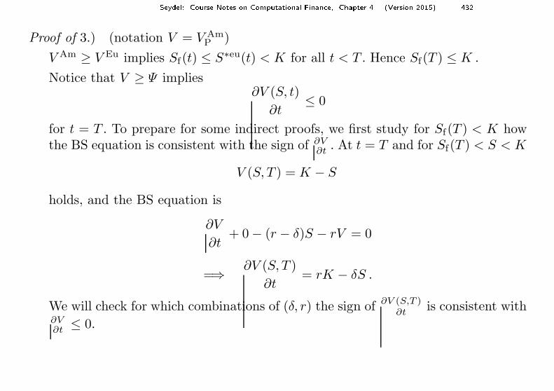
Proof of 3.) (notation V = V AmP )
V Am ≥ V Eu implies Sf(t) ≤ S∗eu(t) < K for all t < T . Hence Sf(T ) ≤ K .
Notice that V ≥ Ψ implies∂V (S, t)
∂t≤ 0
for t = T . To prepare for some indirect proofs, we first study for Sf(T ) < K howthe BS equation is consistent with the sign of ∂V
∂t. At t = T and for Sf(T ) < S < K
V (S, T ) = K − S
holds, and the BS equation is
∂V
∂t+ 0 − (r − δ)S − rV = 0
=⇒ ∂V (S, T )
∂t= rK − δS .
We will check for which combinations of (δ, r) the sign of ∂V (S,T )∂t
is consistent with∂V∂t
≤ 0.
Seydel: Course Notes on Computational Finan e, Chapter 4 (Version 2015) 433
Case δ > r
Here rδK < K. Then either Sf(T ) = r
δK (the assertion), or there exists one of two
open intervals (i) Sf(T ) < rδK and (ii) r
δK < Sf(T ).
(i) For S in the interval Sf(T ) < S < rδK we have ∂V (S,T )
∂t= rK − δS > 0, a
contradiction to∂V
∂t≤ 0 .
(ii) For S in the interval rδK < S < Sf(T ) there is a small dt such that (S, T − dt)
is in the stopping area. The inequality rK < δS holds, and thus
K(erdt − 1) < S(eδdt − 1) ,
since S < K. This means that in case of stopping the dividend yield is largerthan the return of investing K at the risk-free rate. Hence early exercise is notoptimal, which is in conflict with the meaning of S < Sf(t).
Hence Sf(T ) = rδK holds in case δ > r.

Seydel: Course Notes on Computational Finan e, Chapter 4 (Version 2015) 434
Case δ ≤ r
Assume Sf(T ) < K. Then for S in the interval Sf(T ) < S < K a contradiction isobtained from
∂V
∂t︸︷︷︸
≤0
= rK − δS︸ ︷︷ ︸
>0
.
For a call with δ > 0 but without discrete dividend:
1.) Sf(t) is continuously differentiable for t < T .
2.) Sf(t) is monotonic decreasing.
3.)
Sf(T ) := limt→T
t<T
Sf(t) = max{
K,r
δK}
Remark: In case of discrete dividend payment the above assertions must be modified.In particular, Sf then is not continuous! For example, for an American put earlyexercise is not optimal within a certain time interval before ex-dividend date.
Seydel: Course Notes on Computational Finan e, Chapter 4 (Version 2015) 435
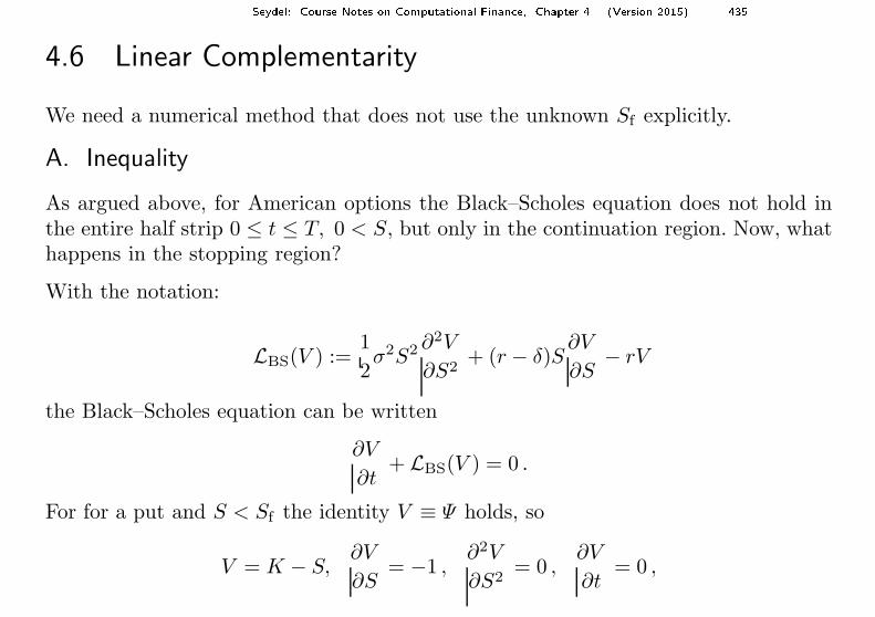
4.6 Linear Complementarity
We need a numerical method that does not use the unknown Sf explicitly.
A. Inequality
As argued above, for American options the Black–Scholes equation does not hold inthe entire half strip 0 ≤ t ≤ T, 0 < S, but only in the continuation region. Now, whathappens in the stopping region?
With the notation:
LBS(V ) :=1
2σ2S2 ∂2V
∂S2+ (r − δ)S
∂V
∂S− rV
the Black–Scholes equation can be written
∂V
∂t+ LBS(V ) = 0 .
For for a put and S < Sf the identity V ≡ Ψ holds, so
V = K − S,∂V
∂S= −1 ,
∂2V
∂S2= 0 ,
∂V
∂t= 0 ,
Seydel: Course Notes on Computational Finan e, Chapter 4 (Version 2015) 436
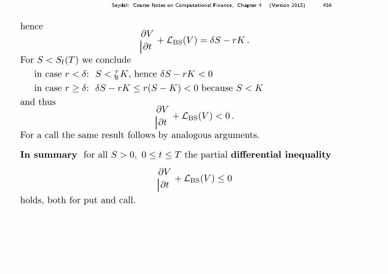
hence∂V
∂t+ LBS(V ) = δS − rK .
For S < Sf(T ) we conclude
in case r < δ: S < rδK, hence δS − rK < 0
in case r ≥ δ: δS − rK ≤ r(S − K) < 0 because S < K
and thus∂V
∂t+ LBS(V ) < 0 .
For a call the same result follows by analogous arguments.
In summary for all S > 0, 0 ≤ t ≤ T the partial differential inequality
∂V
∂t+ LBS(V ) ≤ 0
holds, both for put and call.
Seydel: Course Notes on Computational Finan e, Chapter 4 (Version 2015) 437
Overviewput: V Am
P = K − S for S ≤ Sf
V AmP solves the BS equation for S > Sf
contact condition:∂V (Sf , t)
∂S= −1
call: V AmC = S − K for S ≥ Sf
V AmC solves the BS equation for S < Sf
contact condition:∂V (Sf , t)
∂S= 1
The second derivative of V with respect to S is not continuous at Sf . That is, thevalue function V is smooth in the interior of the continuation region, but not on theentire half strip.
Remark: The transformation of Section 4.1 leads to
∂V
∂t+ LBS(V ) = −∂y
∂τ+
∂2y
∂x2.
Seydel: Course Notes on Computational Finan e, Chapter 4 (Version 2015) 438
B. Formulation with Penalty Term
A unified treatment of ∂V∂t
+ LBS(V ) ≤ 0 on the entire half strip is possible. To thisend, introduce a suitable function p(V ) ≥ 0 requiring the penalty PDE
∂V
∂t+ LBS(V ) + p(V ) = 0
to hold. The penalty term p should be 0 in the continuation region, and positive in thestopping region. The distance to Sf is not known, but the distance V − Ψ of V to thepayoff Ψ is available and is used as control. One example of a penalty function is
p(V ) :=ǫ
V − Ψfor a small ǫ > 0 .
Let Vǫ(S, t) denote the solution of the penalty PDE. Two extreme cases characterizethe effect of the penalty term for (S, t) in the continuation area and in the stoppingarea:
• Vǫ − Ψ ≫ ǫ implies p ≈ 0. Then essentially the Black–Scholes equation results.
• 0 < Vǫ − Ψ ≪ ǫ implies a large value of p, which means that the BS-part of theequation is dominated by p. The BS equation is switched off, and Vǫ ≈ Ψ .
Seydel: Course Notes on Computational Finan e, Chapter 4 (Version 2015) 439
The corresponding branches of the solution Vǫ may be called the “continuation branch”(p ≈ 0) and the “stopping branch” (Vǫ ≈ Ψ). Obviously these two branches appro-ximate the true solution V of the Black–Scholes problem. The intermediate rangeVǫ − Ψ ≈ O(ǫ) characterizes a boundary layer between the continuation branch andthe stopping branch. In this layer around the early-exercise curve Sf the solution Vǫ
can be seen as a connection between the BS surface and the payoff plane.a
Remarks: p and the resulting PDE are nonlinear in V . An implementation thatavoids Vǫ ≤ Ψ is not easy; not every choice of ǫ or ∆t will be successful.
Penalty methods are powerful in general. But for the relatively simple situation ofthe single-asset American option, a more elegant solution is possible. We shall describethis approach next.
a This is illustrated in Topic 9, see the Topics for CF on the homepage www.compfin.de;Topic 9 also also illustrates the penalty function p.
Seydel: Course Notes on Computational Finan e, Chapter 4 (Version 2015) 440
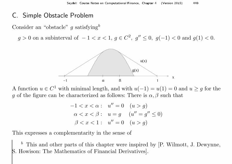
C. Simple Obstacle Problem
Consider an “obstacle” g satisfyingb
g > 0 on a subinterval of − 1 < x < 1, g ∈ C2, g′′ ≤ 0, g(−1) < 0 and g(1) < 0.
g(x)
α βx
u(x)
1−1
A function u ∈ C1 with minimal length, and with u(−1) = u(1) = 0 and u ≥ g for theg of the figure can be characterized as follows: There is α, β such that
−1 < x < α : u′′ = 0 (u > g)
α < x < β : u = g (u′′ = g′′ ≤ 0)
β < x < 1 : u′′ = 0 (u > g)
This expresses a complementarity in the sense of
b This and other parts of this chapter were inspired by [P. Wilmott, J. Dewynne,S. Howison: The Mathematics of Financial Derivatives].
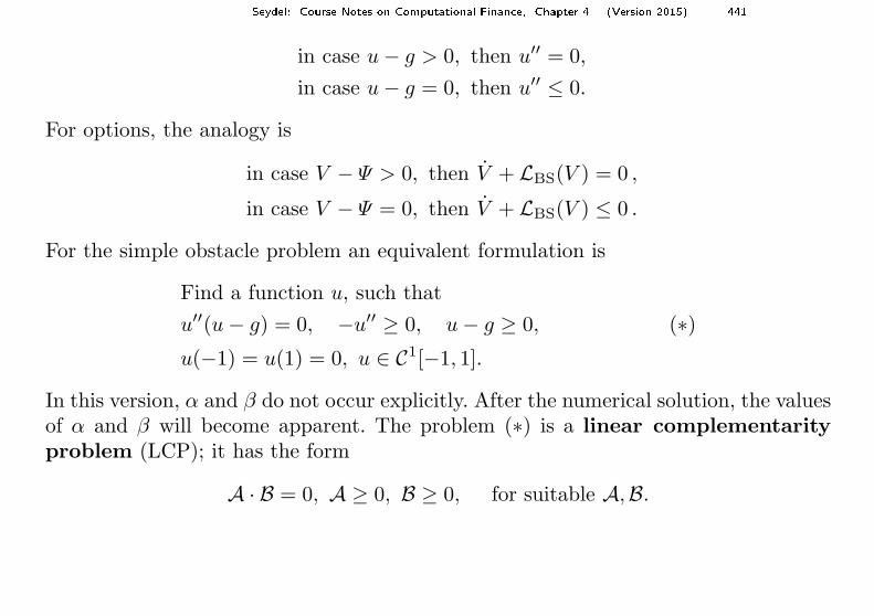
Seydel: Course Notes on Computational Finan e, Chapter 4 (Version 2015) 441
in case u − g > 0, then u′′ = 0,
in case u − g = 0, then u′′ ≤ 0.
For options, the analogy is
in case V − Ψ > 0, then V + LBS(V ) = 0 ,
in case V − Ψ = 0, then V + LBS(V ) ≤ 0 .
For the simple obstacle problem an equivalent formulation is
Find a function u, such that
u′′(u − g) = 0, −u′′ ≥ 0, u − g ≥ 0, (∗)u(−1) = u(1) = 0, u ∈ C1[−1, 1].
In this version, α and β do not occur explicitly. After the numerical solution, the valuesof α and β will become apparent. The problem (∗) is a linear complementarityproblem (LCP); it has the form
A · B = 0, A ≥ 0, B ≥ 0, for suitable A,B.
Seydel: Course Notes on Computational Finan e, Chapter 4 (Version 2015) 442
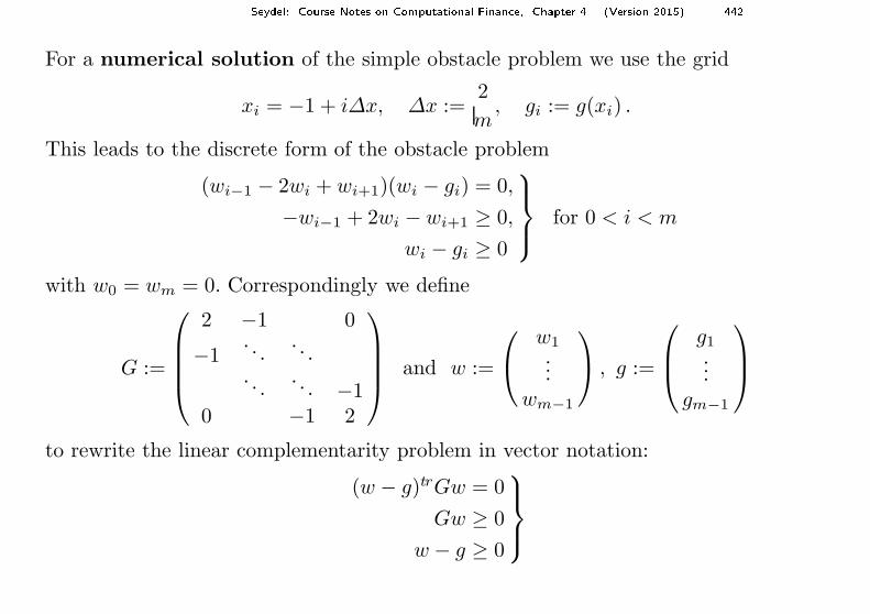
For a numerical solution of the simple obstacle problem we use the grid
xi = −1 + i∆x, ∆x :=2
m, gi := g(xi) .
This leads to the discrete form of the obstacle problem
(wi−1 − 2wi + wi+1)(wi − gi) = 0,
−wi−1 + 2wi − wi+1 ≥ 0,
wi − gi ≥ 0
for 0 < i < m
with w0 = wm = 0. Correspondingly we define
G :=
2 −1 0
−1. . .
. . .. . .
. . . −10 −1 2
and w :=
w1...
wm−1
, g :=
g1...
gm−1
to rewrite the linear complementarity problem in vector notation:
(w − g)trGw = 0
Gw ≥ 0
w − g ≥ 0
Seydel: Course Notes on Computational Finan e, Chapter 4 (Version 2015) 443
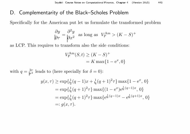
D. Complementarity of the Black–Scholes Problem
Specifically for the American put let us formulate the transformed problem
∂y
∂τ=
∂2y
∂x2as long as V Am
P > (K − S)+
as LCP. This requires to transform also the side conditions:
V AmP (S, t) ≥ (K − S)+
= K max{1 − ex, 0}
with q = 2rσ2 leads to (here specially for δ = 0):
y(x, τ) ≥ exp{12(q − 1)x + 1
4(q + 1)2τ}max{1 − ex, 0}
= exp{14 (q + 1)2τ}max{(1 − ex)e
1
2(q−1)x, 0}
= exp{14 (q + 1)2τ}max{e 1
2(q−1)x − e
1
2(q+1)x, 0}
=: g(x, τ).
Seydel: Course Notes on Computational Finan e, Chapter 4 (Version 2015) 444
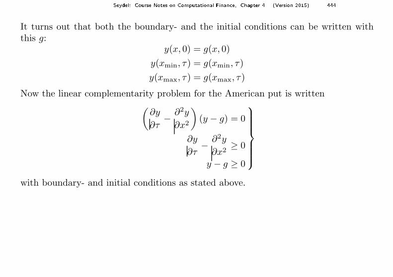
It turns out that both the boundary- and the initial conditions can be written withthis g:
y(x, 0) = g(x, 0)
y(xmin, τ) = g(xmin, τ)
y(xmax, τ) = g(xmax, τ)
Now the linear complementarity problem for the American put is written(
∂y
∂τ− ∂2y
∂x2
)
(y − g) = 0
∂y
∂τ− ∂2y
∂x2≥ 0
y − g ≥ 0
with boundary- and initial conditions as stated above.
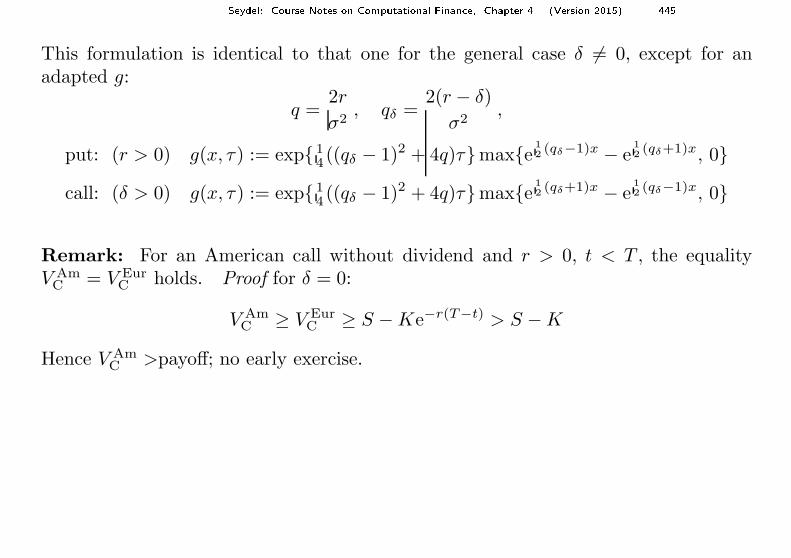
Seydel: Course Notes on Computational Finan e, Chapter 4 (Version 2015) 445
This formulation is identical to that one for the general case δ 6= 0, except for anadapted g:
q =2r
σ2, qδ =
2(r − δ)
σ2,
put: (r > 0) g(x, τ) := exp{14 ((qδ − 1)2 + 4q)τ}max{e 1
2(qδ−1)x − e
1
2(qδ+1)x, 0}
call: (δ > 0) g(x, τ) := exp{14 ((qδ − 1)2 + 4q)τ}max{e 1
2(qδ+1)x − e
1
2(qδ−1)x, 0}
Remark: For an American call without dividend and r > 0, t < T , the equalityV Am
C = V EurC holds. Proof for δ = 0:
V AmC ≥ V Eur
C ≥ S − Ke−r(T−t) > S − K
Hence V AmC >payoff; no early exercise.
Seydel: Course Notes on Computational Finan e, Chapter 4 (Version 2015) 446
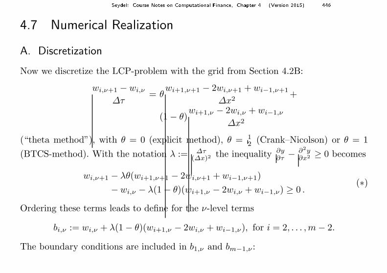
4.7 Numerical Realization
A. Discretization
Now we discretize the LCP-problem with the grid from Section 4.2B:
wi,ν+1 − wi,ν
∆τ= θ
wi+1,ν+1 − 2wi,ν+1 + wi−1,ν+1
∆x2+
(1 − θ)wi+1,ν − 2wi,ν + wi−1,ν
∆x2
(“theta method”), with θ = 0 (explicit method), θ = 12 (Crank–Nicolson) or θ = 1
(BTCS-method). With the notation λ := ∆τ(∆x)2
the inequality ∂y∂τ
− ∂2y∂x2 ≥ 0 becomes
wi,ν+1 − λθ(wi+1,ν+1 − 2wi,ν+1 + wi−1,ν+1)
− wi,ν − λ(1 − θ)(wi+1,ν − 2wi,ν + wi−1,ν) ≥ 0 .(∗)
Ordering these terms leads to define for the ν-level terms
bi,ν := wi,ν + λ(1 − θ)(wi+1,ν − 2wi,ν + wi−1,ν), for i = 2, . . . ,m − 2.
The boundary conditions are included in b1,ν and bm−1,ν :
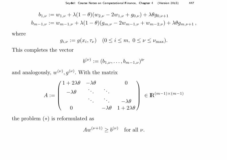
Seydel: Course Notes on Computational Finan e, Chapter 4 (Version 2015) 447
b1,ν := w1,ν + λ(1 − θ)(w2,ν − 2w1,ν + g0,ν) + λθg0,ν+1
bm−1,ν := wm−1,ν + λ(1 − θ)(gm,ν − 2wm−1,ν + wm−2,ν) + λθgm,ν+1 ,
wheregi,ν := g(xi, τν) (0 ≤ i ≤ m, 0 ≤ ν ≤ νmax).
This completes the vector
b(ν) := (b1,ν , . . . , bm−1,ν)tr
and analogously, w(ν), g(ν). With the matrix
A :=
1 + 2λθ −λθ 0
−λθ. . .
. . .. . .
. . . −λθ0 −λθ 1 + 2λθ
∈ IR(m−1)×(m−1)
the problem (∗) is reformulated as
Aw(ν+1) ≥ b(ν) for all ν.
Seydel: Course Notes on Computational Finan e, Chapter 4 (Version 2015) 448
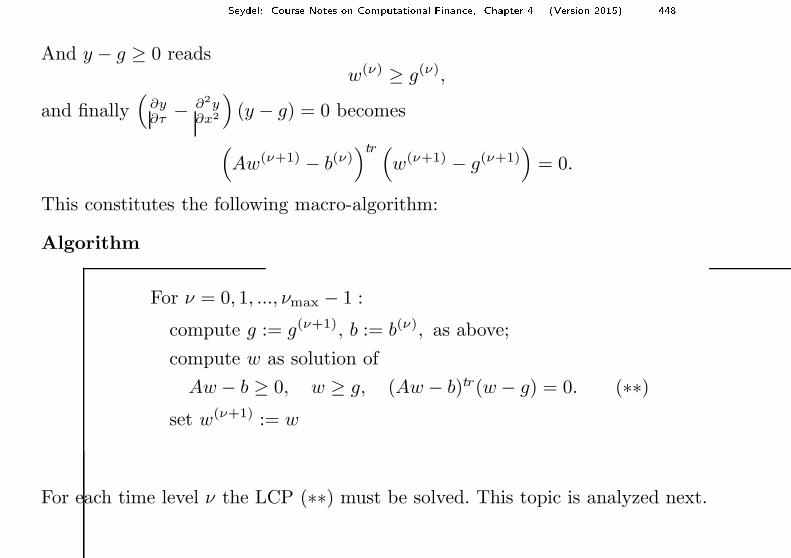
And y − g ≥ 0 readsw(ν) ≥ g(ν),
and finally(
∂y∂τ
− ∂2y∂x2
)
(y − g) = 0 becomes
(
Aw(ν+1) − b(ν))tr (
w(ν+1) − g(ν+1))
= 0.
This constitutes the following macro-algorithm:
Algorithm
For ν = 0, 1, ..., νmax − 1 :
compute g := g(ν+1), b := b(ν), as above;
compute w as solution of
Aw − b ≥ 0, w ≥ g, (Aw − b)tr(w − g) = 0. (∗∗)set w(ν+1) := w
For each time level ν the LCP (∗∗) must be solved. This topic is analyzed next.
Seydel: Course Notes on Computational Finan e, Chapter 4 (Version 2015) 449
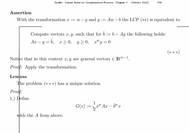
Assertion
With the transformation x := w−g and y := Aw− b the LCP (∗∗) is equivalent to
Compute vectors x, y, such that for b := b − Ag the following holds:
Ax − y = b, x ≥ 0, y ≥ 0, xtry = 0
(∗ ∗ ∗)Notice that in this context x, y are general vectors ∈ IRm−1.
Proof: Apply the transformation.
Lemma
The problem (∗ ∗ ∗) has a unique solution.
Proof:
1.) Define
G(x) :=1
2xtrAx − btrx
with the A from above,
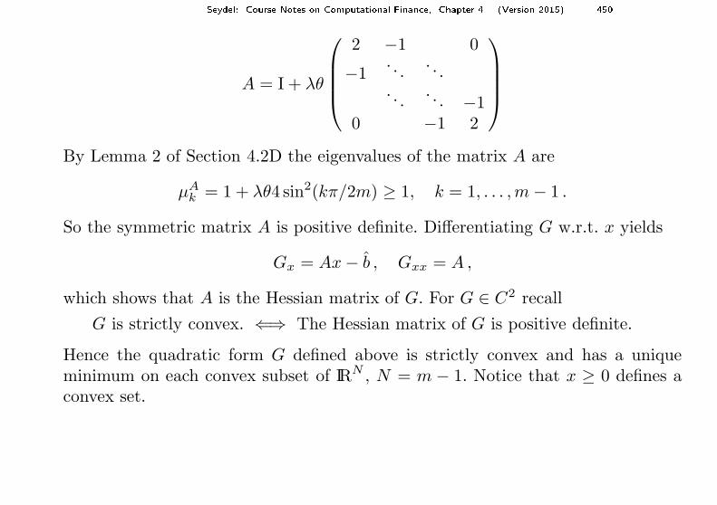
Seydel: Course Notes on Computational Finan e, Chapter 4 (Version 2015) 450
A = I + λθ
2 −1 0
−1. . .
. . .. . .
. . . −10 −1 2
By Lemma 2 of Section 4.2D the eigenvalues of the matrix A are
µAk = 1 + λθ4 sin2(kπ/2m) ≥ 1, k = 1, . . . ,m − 1 .
So the symmetric matrix A is positive definite. Differentiating G w.r.t. x yields
Gx = Ax − b , Gxx = A ,
which shows that A is the Hessian matrix of G. For G ∈ C2 recall
G is strictly convex. ⇐⇒ The Hessian matrix of G is positive definite.
Hence the quadratic form G defined above is strictly convex and has a uniqueminimum on each convex subset of IRN , N = m − 1. Notice that x ≥ 0 defines aconvex set.
Seydel: Course Notes on Computational Finan e, Chapter 4 (Version 2015) 451
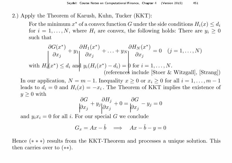
2.) Apply the Theorem of Karush, Kuhn, Tucker (KKT):
For the minimum x∗ of a convex function G under the side conditions Hi(x) ≤ di
for i = 1, . . . , N , where Hi are convex, the following holds: There are yi ≥ 0such that
∂G(x∗)
∂xj
+ y1∂H1(x
∗)
∂xj
+ . . . + yN
∂HN (x∗)
∂xj
= 0 (j = 1, . . . , N)
with Hi(x∗) ≤ di and yi(Hi(x
∗) − di) = 0 for i = 1, . . . , N .(references include [Stoer & Witzgall], [Strang])
In our application, N = m − 1. Inequality x ≥ 0 or xi ≥ 0 for all i = 1, . . . ,m − 1leads to di = 0 and Hi(x) = −xi . The Theorem of KKT implies the existence ofy ≥ 0 with
∂G
∂xj
+ yj
∂Hj
∂xj
+ 0 =∂G
∂xj
− yj = 0
and yixi = 0 for all i. For our special G we conclude
Gx = Ax − b =⇒ Ax − b − y = 0
Hence (∗ ∗ ∗) results from the KKT-Theorem and processes a unique solution. Thisthen carries over to (∗∗).

Seydel: Course Notes on Computational Finan e, Chapter 4 (Version 2015) 452
B. Numerical Solution
A direct solution of (∗∗) is possible. Brennan & Schwartz suggest to proceed as follows:
Solve Aw = b componentwise such that
the side condition w ≥ g is obeyed.
This is a somewhat vague outline of an approach: the implementation matters. It isbased on the Gaussian elimination, which in its first phase transforms Aw = b into anequivalent system Aw = b, so that A is a triangular matrix (here bidiagonal). Then,in the second phase, the above principle of Brennan & Schwartz can be solved withone loop. When A is upper triangular, then this loop to solve Aw = b is a backwardrecursion. For a lower triangle A, the loop is forward. If in the ith step of the loop wi
denotes the component of the solution of Aw = b, then wi := max{wi, gi} appears tobe a realization.
But w depends on the loop’s order. Only one direction works. An implementationmust make sure that the characteristic structure of the option is matched.
Seydel: Course Notes on Computational Finan e, Chapter 4 (Version 2015) 453
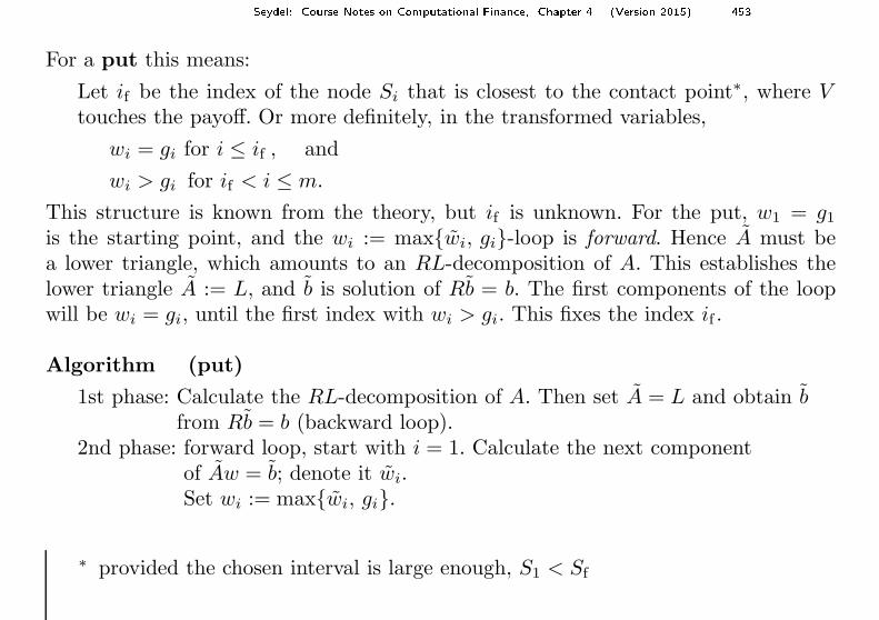
For a put this means:
Let if be the index of the node Si that is closest to the contact point∗, where Vtouches the payoff. Or more definitely, in the transformed variables,
wi = gi for i ≤ if , and
wi > gi for if < i ≤ m.
This structure is known from the theory, but if is unknown. For the put, w1 = g1
is the starting point, and the wi := max{wi, gi}-loop is forward. Hence A must bea lower triangle, which amounts to an RL-decomposition of A. This establishes thelower triangle A := L, and b is solution of Rb = b. The first components of the loopwill be wi = gi, until the first index with wi > gi. This fixes the index if .
Algorithm (put)
1st phase: Calculate the RL-decomposition of A. Then set A = L and obtain bfrom Rb = b (backward loop).
2nd phase: forward loop, start with i = 1. Calculate the next componentof Aw = b; denote it wi.Set wi := max{wi, gi}.
∗ provided the chosen interval is large enough, S1 < Sf
Seydel: Course Notes on Computational Finan e, Chapter 4 (Version 2015) 454
The costs are low (solution of a linear system with tridiagonal matrix). It can beshown that the above procedure for a standard option with the underlying matrix Aworks well.
For a call (δ > 0) one proceeds the other way: The loop starts with wm = gm andthe second phase is a backward loop. To make this possible, in the first phase the“traditional” LR-decomposition of A establishes an upper triangle A = R, and b isobtained from Lb = b in a foward loop.
Remark on the accuracy:
Since V (S, t) fails to be twice continuously differentiable w.r.t. S at Sf(t), we expectsome bad influence on the accuracy. (Recall that Crank–Nicolson even assumesy ∈ C4.) But in spite of this lack of smoothness, the Crank–Nicolson approach hereis sufficiently accurate, oscillations diminish rapidly. The lack of smoothness in thepayoff is worse. Even extrapolation works rather well, although the assumptions ofsmoothness are not satisfied.
Seydel: Course Notes on Computational Finan e, Chapter 4 (Version 2015) 455
Outlook
This concludes the introduction in basic Computational Finance. An essential part ofthe course are the exercises and the programming assignments.
If this is the material for one semester, then there will be more time left for someadditional topics. (In my course, typically, there are two weeks left.) This additionalmaterial is not included in these course notes, because it will differ from course tocourse, depending on the interests and the knowledge of the students. For a textbookexplaining additional material, see [Seydel: Tools for Computational Finance, sixthEdition (2017)], from which we take the following section numbers. Possible topicsinclude
• an analytic method: interpolation (§4.8.1), or integral equation (§4.8.4)
• upwind scheme and its relevance (§6.4 – 6.5)
• a penalty method in the two-dimensional case (§6.7)
• case studies, such as the two-dimensional tree method of Exercise 6.2
• jump diffusion (§1.9, §7.3)
and for a two-semester course or an accompanying seminar, one may address
• finite elements (Chapter 5)

Seydel: Course Notes on Computational Finan e, Chapter 4 (Version 2015) 456
• nonlinear Black–Scholes problems (§7.1 – 7.2)