Cosmology & CMB

Set6: Polarisation&

Secondary Anisotropies

Davide Maino

Polarisation

• How? Polarisation is generated via Compton/Thomsonscattering (angular dependence of the scattering termM)

• Who? Only quadrupole anisotropy is able to produce linearpolarisation

• When? Near recombination Θ2 is at 5-10% level of Θ0

Polarisation

• Linear polarisation is described by Stokes Q and U parameters• Q measures differences of intensities along the x and y axes,

while U measures same differences but in a 45 rotated frame• Stokes are not in general rotationally invariant

Q′ = Qcos(2ψ)− Usin(2ψ) U′ = Ucos(2ψ) + Qsin(2ψ)

Q′ ± iU′ = e±2iψ(Q± iU)

• (Q± iU) transform like a spin-2 tensor

Polarisation: Spin weighted spherical harmonics

• A general spin-2 tensor on a sphere is properly represented byspin-s spherical harmonics sY`m

• Under rotation: sY`m → e±isψsY`m

• Normality and completeness∫dn sY?`m(n) sY`′m′(n) = δ``′δmm′∑`m

sY?`m(n) sY`m(n′) = δ(φ− φ′)δ(cosθ − cos(θ′)

Polarisation: All-sky decomposition

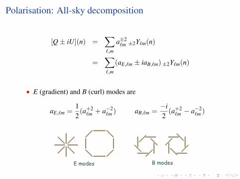
[Q± iU](n) =∑`,m

a±2`m ±2Y`m(n)

=∑`,m

(aE,`m ± iaB,`m)±2Y`m(n)

• E (gradient) and B (curl) modes are

aE,`m =12

(a+2`m + a−2

`m ) aB,`m =−i2

(a+2`m − a−2

`m )

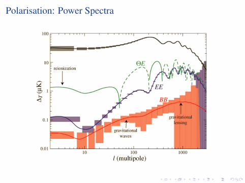
Polarisation: Power Spectra

• Four parity-independent power spectra

CTT =1

2`+ 1

∑m

〈a?T,`maT,`m〉 CTE =1

2`+ 1

∑m

〈a?T,`maE,`m〉

CEE =1

2`+ 1

∑m

〈a?E,`maE,`m〉 CBB =1

2`+ 1

∑m

〈a?B,`maB,`m〉

• E-modes are generated by both scalar (density) and tensor (gw)perturbation

• B-modes are generated only by tensor perturbation: direct probeof inflation

Polarisation: Power Spectra

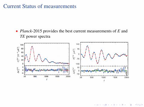
Current Status of measurements

• Planck-2015 provides the best current measurements of E andTE power spectra

Secondary Anisotropies

• CMB photons traverse the large-scale structure of the Universefrom z ∼ 1000 to the present

• Having nearly scale-invariant adiabatic fluctuations (from CMBobservations), structures form bottom-up i.e. small scales first.Hierarchical structure formation.

• First objects (starts) re-ionize the Universe between z ∼ 7÷ 30• Gravitational: Integrated Sach-Wolfe effect (ISW), gravitational

lensing• Scattering: peak suppression, large-angle polarisation (Compton

scattering)

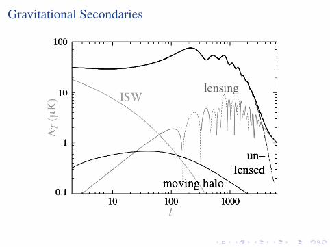
Gravitational Secondaries

Transfer Function

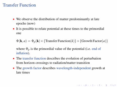
• We observe the distribution of matter predominantly at lateepochs (now)

• It is possible to relate potential at these times to the primordialone

Φ(k, a) = Φp(k)×Transfer Function(k)×Growth Factor(a)

where Φp is the primordial value of the potential (i.e. end ofinflation).

• The transfer function describes the evolution of perturbationfrom horizon crossings to radiation/matter transition

• The growth factor describes wavelength-independent growth atlate times

Transfer Function

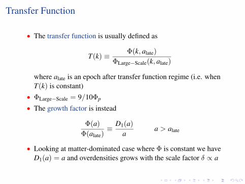
• The transfer function is usually defined as

T(k) ≡ Φ(k, alate)

ΦLarge−Scale(k, alate)

where alate is an epoch after transfer function regime (i.e. whenT(k) is constant)

• ΦLarge−Scale = 9/10Φp

• The growth factor is instead

Φ(a)

Φ(alate)≡ D1(a)

aa > alate

• Looking at matter-dominated case where Φ is constant we haveD1(a) = a and overdensities grows with the scale factor δ ∝ a

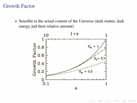
Growth Factor

• Sensible to the actual content of the Universe (dark matter, darkenergy and their relative amount)

Integrated Sachs-Wolfe (ISW) effect

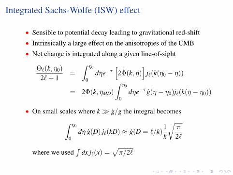
• Sensible to potential decay leading to gravitational red-shift• Intrinsically a large effect on the anisotropies of the CMB• Net change is integrated along a given line-of-sight

Θ`(k, η0)

2`+ 1=

∫ η0

0dηe−τ

[2Φ(k, η)

]j`(k(η0 − η))

= 2Φ(k, ηMD)

∫ η0

0dηe−τ g(η − η0)j`(k(η − η0))

• On small scales where k g/g the integral becomes∫ η0

0dη g(D) j`(kD) ≈ g(D = `/k)

1k

√π

2`

where we used∫

dx j`(x) =√π/2`

Integrated Sachs-Wolfe (ISW) effect

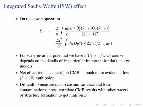
• On the power spectrum

C` =2π

∫dkk

k3〈Θ?` (k, η0)Θ`(k, η0)〉

(2`+ 1)2

=2π2

`3

∫dηDg2(η)∆2

Φ(`/D, ηMD)

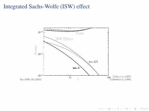
• For scale-invariant potential we have `2C` ∝ 1/`. Of coursedepends on the details of g: particular important for dark energymodels

• Net effect (enhancement) on CMB is much more evident at low(` < 10) multipoles

• Difficult to measure due to cosmic variance and localcontaminations: cross-correlate CMB results with other tracersof structure formation to get hints on D1

Integrated Sachs-Wolfe (ISW) effect

Integrated Sachs-Wolfe (ISW) effect

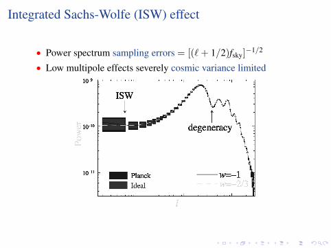
• Power spectrum sampling errors = [(`+ 1/2)fsky]−1/2

• Low multipole effects severely cosmic variance limited

Gravitational Lensing

• Lensing is a remapping conserving surface brightness of sourceimage reprojected via the gradient of a projected potential

φ(n) = 2∫ η0

η?

dη(D? − D)

DD?Φ(Dn, η)

such that fields are re-mapped as

x(n)→ x(n +∇φ)

where x ∈ Θ,Q,U temperature and polarization• Taylor expansion leads to product of fields and Fourier

mode-coupling

Flat-sky Treatment

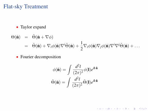
• Taylor expand

Θ(n) = Θ(n +∇φ)

= Θ(n) +∇iφ(n)∇iΘ(n) +12∇iφ(n)∇jφ(n)∇i∇jΘ(n) + . . .

• Fourier decomposition

φ(n) =

∫d2l

(2π)2φ(l)eil·n

Θ(n) =

∫d2l

(2π)2 Θ(l)eil·n

Flat-sky Treatment

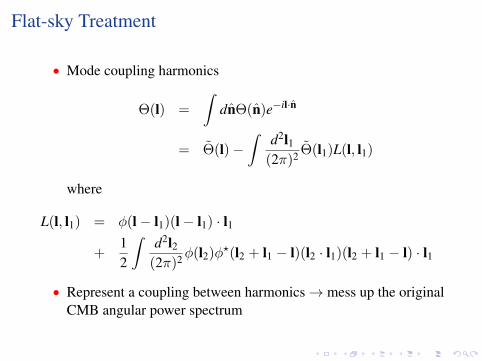
• Mode coupling harmonics

Θ(l) =

∫dnΘ(n)e−il·n

= Θ(l)−∫

d2l1(2π)2 Θ(l1)L(l, l1)

where

L(l, l1) = φ(l− l1)(l− l1) · l1

+12

∫d2l2

(2π)2φ(l2)φ?(l2 + l1 − l)(l2 · l1)(l2 + l1 − l) · l1

• Represent a coupling between harmonics→ mess up the originalCMB angular power spectrum

Power Spectrum

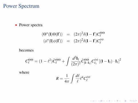
• Power spectra

〈Θ?(l)Θ(l′)〉 = (2π)2δ(l− l′)CΘΘ`

〈φ?(l)φ(l′)〉 = (2π)2δ(l− l′)Cφφ`

becomes

CΘΘ` = (1− `2)CΘΘ

` +

∫d2l1

(2π)2 CΘΘ|l−l1|C

φφ`1

[(l− l1) · l1]2

whereR =

14π

∫d```4Cφφ`

Smoothing of Power Spectra

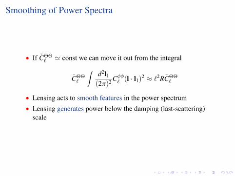
• If CΘΘ` ' const we can move it out from the integral

CΘΘ`

∫d2l1

(2π)2 Cφφ` (l · l1)2 ≈ `2RCΘΘ`

• Lensing acts to smooth features in the power spectrum• Lensing generates power below the damping (last-scattering)

scale

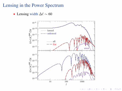
Lensing in the Power Spectrum

• Lensing width ∆` ∼ 60

l(l+

1)C

l /2π

ΘΘ

l(l+

1)C

l /2π

ΘΕ

l

10–9

10–10

10–11

10–12

10–13

10–11

10–12

10–13

10–14

10–15

10 100 1000

lensed

unlensed

all

flat

error

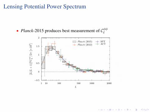
Lensing Potential Power Spectrum

• Planck-2015 produces best measurement of Cφφ`

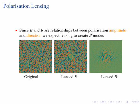
Polarisation Lensing

• Since E and B are relationships between polarisation amplitudeand direction we expect lensing to create B modes

Original Lensed E Lensed B

Polarisation Lensing

• Polarisation field harmonics lensed similarly

[Q± iU](n) = −∫

d2l(2π)2 [E ± iB] (l)e±2iφlel·n

• Again with Taylor expansion

[Q± iU](n) = [Q± iU](n +∇φ)

≈ [Q± iU](n) +∇iφ(n)∇i[Q± iU](n)

+12∇iφ(n)∇jφ(n)∇i∇j[Q± iU](n)

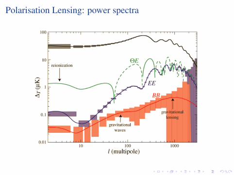
Polarisation Lensing: power spectra

• In terms of power spectra (Zaldarriaga & Seljak 98)

CTT = CTT +W l′1`CTT

CEE = CEE +12

[W`′

1` +W`′2`

]CEE +

12

[W`′

1` −W`′2`

]CBB

CBB = CBB +12

[W`′

1` −W`′2`

]CEE −

12

[W`′

1` +W`′2`

]CEE

CTE = CTE +W`′3`CTE

• Lensing mixes E and B modes: even with no primordial GW,B-modes are generated at small scales

Polarisation Lensing: power spectra

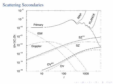
Scattering Secondaries

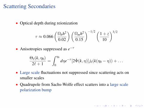
Scattering Secondaries

• Optical depth during reionization

τ ≈ 0.066(

Ωbh2

0.02

)(Ωmh2

0.15

)−1/2(1 + z10

)3/2

• Anisotropies suppressed as e−τ

Θ`(k, η0)

2`+ 1=

∫ η0

0dηe−τ [2Φ(k, η)] j`(k(η0 − η)) + . . .

• Large scale fluctuations not suppressed since scattering acts onsmaller scales

• Quadrupole from Sachs-Wolfe effect scatters into a large scalepolarization bump

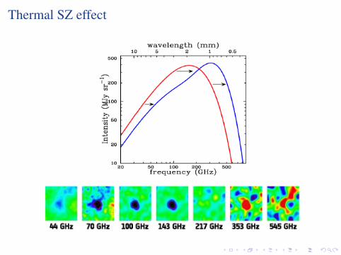
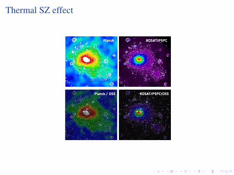
Thermal SZ effect

• Thermal velocities lead to Doppler effect but cancels out at firstorder due to random directions

• Residual effect of the order v2τ ≈ Te/meτ and could beimportant for Te ≈ 10keV (gas within cluster of galaxies)

• RJ decrement and Wien enhancement described by second ordercollision term in Boltzmann equation: Kompaneets equation

• Clusters are rare objects so contribution to power spectrumsuppressed but has been detected already by Planck: sensitive to(matter) power spectrum normalization σ8

Thermal SZ effect

Thermal SZ effect

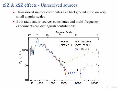
tSZ & kSZ effects - Unresolved sources• Un-resolved sources contributes as a background noise on very

small angular scales• Both radio and ir-sources contributes and multi-frequency

experiments can distinguish contributions

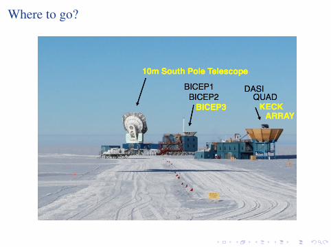
Where to go?

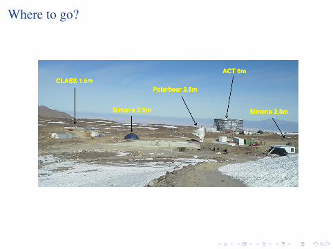
Where to go?