CORPUS AND TEXT PROCESSING FOR LANGUAGE TEACHING : ON-LINE

RESEARCH Open Access

Oscillating global continua of positive solutionsof second order Neumann problem with a set-valued termDongming Yan

Correspondence:[email protected] of Mathematics,Sichuan University, Chengdu610064, China

Abstract

In this note, we study the oscillating global continua of the differential inclusion ofthe form{−u′′ + qu ∈ λF(·, u),

u′(0) = 0, u′(1) = 0,

where F is a “set-valued representation” of a function with jump discontinuities alongthe line segment [0, 1] × {0}, and l Î [0, ∞) is a parameter. The proof of our mainresult relies on an approximation procedure.Mathematics Subject Classification 2000: 34B16; 34B18.

Keywords: climate model, differential inclusion, eigenvalue, positive solutions

1 IntroductionIn recent years, nonsmooth analysis has come to play an important role in functional

analysis [1], dynamical systems [2], control theory [3], optimization [4], mechanical sys-

tems [5], differential equation [6,7] etc. Since many mathematical and physical pro-

blems may be reduced to ODES or PDES with discontinuous nonlinearities, the

existence of multiple solutions for differential inclusion problems has been widely

investigated [8-19].

In this article, we are concerned with the following differential inclusion problem

which raises from a Budyko-North type energy balance climate models:{−u′′(x) + q(x)u(x) ∈ λF(x, u(x)), a.e.x ∈ (0, 1),u′(0) = 0, u′(1) = 0

(1:1)

(see [20-25] and the references therein). In particular, the set-valued right hand side

arise from a jump discontinuity of the albedo at the ice-edge in these models. By filling

such a gap, one arrives at the set-valued problem (1.1). As in [25], we are here inter-

ested in a considerably simplify version as compared to the situation from climate

modeling, e.g. a one-dimensional regular Sturm-Liouville differential operator substi-

tutes for a two-dimensional Laplace-Beltrami operator or a singular Legendre-type

operator, and the jump discontinuity is transformed to u = 0 in a way, which resem-

bles only locally the climatological problem.

Yan Boundary Value Problems 2012, 2012:47http://www.boundaryvalueproblems.com/content/2012/1/47

© 2012 Yan; licensee Springer. This is an Open Access article distributed under the terms of the Creative Commons Attribution License(http://creativecommons.org/licenses/by/2.0), which permits unrestricted use, distribution, and reproduction in any medium, providedthe original work is properly cited.

mailto:[email protected]

http://creativecommons.org/licenses/by/2.0

We are concerned with the set-valued problem (1.1) under the following

assumptions

(H1) qÎC([0, 1],(0,+∞));(H2) f+Î C ([0, 1] × [0,+∞), (0,+∞)),

infx∈[0,1]

f +(x, 0) > 0, lims→+∞

f +(x, s)s

= b(x) ∈ C([0, 1], (0,∞)) .

Let the set-valued function F in (1.1) is given by

F(x, y) ={ {f +(x, y)}, x ∈ [0, 1], y > 0,[0, f +(x, 0)], x ∈ [0, 1].

Notice that if f+(x, 0) ≡ 0, x Î [0, 1], then the differential inclusion problem (1.1)

reduces to the BVP of differential equation{−u′′(x) + q(x)u(x) = λf +(x, u(x)), x ∈ (0, 1),u′(0) = 0, u′(1) = 0.

(1:2)

In the last 20 years, the positive solutions of (1.2) have been studied by several

authors, see Jiang and Liu [26], Chu et al. [27] and Sun et al. [28].

The purpose of this article is to investigate the oscillating global continua of positive

solutions of the differential inclusion problem (1.1). The proof of our main result relies

on an approximation procedure. The rest of the article is organized as follows. In Sec-

tion 2, we state some notations and prove some preliminary results. In Section 3, we

state and prove our main result. In Section 4, an example is given to illustrate the

application of our main result.

2 Notations and preliminariesRecall Kuratowski’s notion of lower and upper limits of sequence of sets.

Definition 2.1. [29]Let X be a metric space and {Zl}lÎNbe a sequence of subsets of X.

The set

lim supl→∞

Zl :={x ∈ X : lim inf

l→∞dist(x,Zl) = 0

}

is called the upper limit of the sequence {Zl}, whereas

lim infl→∞

Zl :={x ∈ X : lim

l→∞dist(x,Zl) = 0

}

is called the lower limit of the sequence {Zl}.

Definition 2.2. [29]A component of a set M is meant a maximal connected subset of

M.

Lemma 2.1. [29]Suppose that Y is a compact metric space, A and B are non-inter-

secting closed subsets of Y, and no component of Y intersects both A and B. Then there

exist two disjoint compact subsets YAand YB, such that Y = YA∪YB, A ⊂ YA, B ⊂ YB.

Using the above Whyburn Lemma, Ma and An [30] proved the following

Lemma 2.2. [30, Lemma 2.1] Let Z be a Banach space and let {An} be a family of

closed connected subsets of Z. Assume that

(i) there exist zn Î An, n = 1, 2, ..., and z* Î Z, such that zn ® z*;

(ii) rn = sup {∥x∥ | x Î An} = ∞;


of 13

(iii) for every R > 0,(⋃∞

n=1 An) ∩ BR is a relatively compact set of Z, where BR= {x Î Z

| ∥x∥ ≤ R}. Then there exists an unbounded component C in lim supl→∞

Al and z∗ ∈ C .

Remark 2.1. The limiting processes for sets go back at least to the work of Kura-

towski [31]. Lemma 2.2 is a slight generalization of the following well-know result due

to Whyburn [29]:

Proposition 2.1. (Whyburn [29, p. 12]) Let Z be a Banach space and {An} be a family

of closed connected subsets of Z. Let lim infl→∞

Al �= ∅ and ∪lÎNAl is relatively compact.

Then lim supl→∞

Al is nonempty, compact and connected.

Next, we introduce the result of global solution behavior of the bifurcation branches

of the equation

x = μ(Lx +Nx), μ ∈ R, x ∈ X, (2:1)

to wit the following lemma.

Lemma 2.3. [32] (Dancer (1974)) Assume that

(C1) The operators L, N: X ® X are compact on the Banach space X over R. Further-

more, L is linear and ∥Nx∥/∥x∥ ® 0 as ∥x∥ ® 0;

(C2) The real number μ0is a characteristic number of L of odd algebraic multiplicity;

(C1+) The real Banach space X has an order cone K with X = K-K, i.e., every x Î X

can be represented as x = x1 - x2, where x1, x2 Î K. Furthermore, L + N is positive, i.e.,

L + N maps K into K;

(C2+) The spectral radius r(L) of L is positive. We set μ0 = (r(L))-1.

Then (μ0, 0) is a bifurcation point of equation (2.1) and

S+ := {(μ, x) ∈ R × X : (μ, x) is a solution of (2.1)withμ > 0, x > 0}

contains an unbounded solution component C+1which passes through (μ0, 0).

If additionally

(C3+) The linear operator L is strongly positive, then (μ, x) ∈ C+1and μ ≠ μ0always

implies x > 0 and μ > 0.

Remark 2.2. This result is often called the nonlinear Krein-Rutman theorem. It will

play an important role in the proof of our main result.

Let � and ψ be the unique solution of the problems{−u′′(x) + q(x)u(x) = 0, x ∈ (0, 1),u′(0) = 0, u(0) = 1

and {−u′′(x) + q(x)u(x) = 0, x ∈ (0, 1),u′(1) = 0, u(1) = 1

respectively. Then it is easy to check �(·) is nondecreasing on (0,1), ψ(·) is nonin-

creasing on (0,1), and the Green’s function G(x, s) of{−u′′(x) + q(x)u(x) = 0, x ∈ (0, 1),u′(0) = 0, u′(1) = 0


of 13

is explicitly given by

G(x, s) = − 1ψ ′(0)

{ψ(x)ϕ(s), 0 ≤ s ≤ x ≤ 1,ϕ(x)ψ(s), 0 ≤ x ≤ s ≤ 1.

(2:2)

Moreover, we have that

0 < G(x, s) ≤ G(s, s), (x, s) ∈ [0, 1] × [0, 1];

σG(s, s) ≤ G(x, s), (x, s) ∈ [0, 1] × [0, 1](2:3)

with σ := min{

1ψ(0)

,1

ϕ(1)

}. .

3 The main resultLet Σ be the closure of the set of positive solutions of (1.1) in [0, ∞) × C1[0, 1], and N*

:= {1, 2,..., N}. The main result of this article is the following theorem.

Theorem 3.1. Assume that (H1)-(H2) hold. If

(H3) there is an increasing sequence of positive numbers{ξj

}N1and a small enough

constant δ such that ξ1 <s(ξ2- δ) and

�(ξ2j−1) <12

⎛⎝ 1∫

0

G(s, s)ds

⎞⎠

−1

(ξ2j−1 − δ), j ∈ N∗;

(ξ2j) > 2

⎛⎝ 1∫

0

G(12, s

)ds

⎞⎠

−1

(ξ2j + δ), j ∈ N∗,

where

�(l) := max{f +(t, c) : 0 ≤ t ≤ 1, 0 ≤ c ≤ l + δ},(l) := min{f +(t, c) : 0 ≤ t ≤ 1, σ (l − δ) ≤ c ≤ l + δ},

then there exits an unbounded component C+1in Σ with (0, 0) ∈ C+

1 . Moreover,

(i) (λ, u) ∈ C+1with ∥u∥∞ = ξ2j-1for some j Î N* implies that l ≥ 2;

(ii) (λ, u) ∈ C+1with ∥u∥∞ = ξ2jfor some j Î N* implies that λ ≤ 1

2.

Actually, such continua C+1 can be obtained as upper limits in the sense of Kura-

towski of sequence of solution continua from associated continuous problems. To this

end one sets

dg := inf{f +(x, 0) : x ∈ [0, 1]}, (3:1)

fixes l0 Î N such thatdgl0

< ξ1 , and selects an approximation sequence {fl} ⊂ C ([0,

1] × ℝ, ℝ) (l >l0) of F satisfying:

(A1) fl (x, y) = ly for x Î [0, 1] and y ∈[0,

dg2l

];

(A2)dg2

≤ fl(x, y) ≤ f +(x, y) for x Î [0, 1] and y ∈[dg2l,dgl

];


of 13

(A3) fl(x,y) = f+(x, y) for x Î [0, 1] and y ≥ dgl;

(A4) {fl (x, y)}lÎN is nondecreasing in l for (x, y) Î [0, 1] × (0,∞).

Next, we show that the continuous problem{−v′′(x) + q(x)v(x) = λfl(x, v(x)), x ∈ (0, 1),v′(0) = 0, v′(1) = 0

(3:2l)

has an unbounded closed subsets C+1,l of the positive solutions set of (3.2l) with

(a)(

λ1

l, 0

)is the bifurcation point contained in C+

1,l ;

(b) If (μ,ϑ) ∈ C+1,l and ϑ ≢ 0, then ϑ is positive on (0,1).

It is easy to see that (3.2l) equivalent to

v(x) = λ

1∫0

G(x, s)fl(s, v(s))ds. (3:3)

Let

(Lv)(x) : = l

1∫0

G(x, s)v(s)ds,

(Nv)(x) : =

1∫0

G(x, s)(fl(s, v(s)) − lv(s))ds, v ∈ C[0, 1].

Then according to (3.3), (3.2l) can be written as the following operator equation

v = λ(Lv +Nv).

Clearly, the operators L, N : C[0, 1] ® C[0, 1] are compact on the Banach space

C[0, 1]. Furthermore, L is linear and thanks to (2.3)(A1) that

‖Nv‖∞‖v‖∞

=

∥∥∥∥∥∥1∫

0

G(x, s)fl(s, v(s)) − lv(s)

‖v‖∞ds

∥∥∥∥∥∥∞

≤1∫

0

G(s, s)

∣∣fl(s, v(s)) − lv(s)∣∣

‖v‖∞ds → 0, as‖v‖∞ → 0,

which implies that the condition (C1) of Lemma 2.3 is satisfied.

Denote the principal eigenvalue of{−ω′′(x) + q(x)ω(x) = λω(x), x ∈ (0, 1),ω′(0) = 0, ω′(1) = 0,

(3:4)

by l1, then we know that l1>0 (see [33]). Since (3.4) is equivalent to operator equa-

tion

ω =λ

lLω,


of 13

we have that (r(L))−1 =λ1

l. Therefore, the conditions (C2)(C2+) of Lemma 2.3 are

satisfied.

Let the cone K in C[0, 1] is given by

K ={u ∈ C[0, 1]

∣∣u(x) ≥ 0, 0 ≤ x ≤ 1}.

It is easy to see thanks to (A1)-(A4) and (2.3) that the (C1+)(C3+) conditions of

Lemma 2.3 are satisfied.

According to Lemma 2.3, we obtain that(

λ1

l, 0

)is a bifurcation point of the posi-

tive solutions set of (3.2l) for every l Î {l0 + 1, l0 + 2, ...} =: N0, and for each l Î N0

there exits an unbounded closed subsets C+1,l of the positive solutions set of (3.2l) with

(a) and (b).

Combining the above with the fact

liml→∞

(λ1

l, 0

)= (0, 0)

and utilizing Lemma 2.2, it concludes that there exits an unbounded component C+1

with

(0,0) ∈ C+1 (3:5)

and

C+1 ⊂ lim sup

l→∞C+1,l. (3:6)

Denote the cone P in C[0, 1] by

P ={u ∈ C[0, 1]

∣∣ min0≤x≤1

u(x) ≥ σ‖u‖∞

}.

Define an operator Tl : P ® C[0, 1] by

(Tλu) (x) = λ

1∫0

G(x, s)fl(s, u(s))ds, x ∈ [0, 1].

It is easy to get the following lemma.

Lemma 3.1. Assume that (H1), (H2) and (A1)-(A4) hold. Then Tl: P ® P is comple-

tely continuous.

Lemma 3.2. Assume that (H1), (H2) and (A1)-(A4) hold. If 0 ≤ u(x) ≤ r, r > 0, for x Î[0, 1], then

‖Tλu‖∞ ≤ λMr

1∫0

G(s, s)ds,

where Mr = max0≤x≤1,0≤s≤r

{fl(x, s)}.


of 13

Proof. Since fl(x, u(x)) ≤ Mr for x Î [0, 1], it follows from (2.3) that

‖Tλu‖∞ =

∥∥∥∥∥∥λ

1∫0

G(x, s)fl(s, u(s))ds

∥∥∥∥∥∥∞

≤ λ

1∫0

G(s, s)fl(s, u(s))ds

≤ λMr

1∫0

G(s, s)ds.

Lemma 3.3. Assume that (H1), (H2) and (A1)-(A4) hold. If s(r - δ) ≤ u(x) ≤ r + δ, r

>δ, for x Î [0, 1], then

‖Tλu‖∞ ≥ λmr

1∫0

G(12, s

)ds,

where mr = min0≤x≤1, σ (r−δ)≤s≤r+δ

{fl(x, s)} .Proof. Since fl(x, u(x)) ≥ mr for x Î [0, 1], it follows that

‖Tλu‖∞ ≥ λ

1∫0

G(12, s

)fl(s, u(s))ds

≥ λmr

1∫0

G(12, s

)ds.

Lemma 3.4. Assume that (H1), (H2), (H3) and (A1)-(A4) hold. then

(i) (λ, u) ∈ C+1,lwith ∥u∥∞ Î (ξ2j-1 - δ,ξ2j-1 + δ) for some j Î N* implies that l > 2;

(ii) (λ, u) ∈ C+1,l , with ∥u∥∞ Î ( ξ2j- δ,ξ2j + δ) for some j Î N* implies that λ <

12.

Proof. (i) Assume that (λ, u) ∈ C+1,l with ∥u∥∞ Î (ξ2j-1 - δ, ξ2j-1 + δ) for some j Î N*,

then u = Tlu and

0 ≤ u(x) ≤ ξ2j−1 + δ for x ∈ [0, 1].

By Lemma 3.2 and (H3), it follows that

‖u‖∞ = ‖Tλu‖∞

≤ λMξ2j−1+δ

1∫0

G(s, s)ds

= λ max0≤x≤1,0≤s≤ξ2j−1+δ

{fl(x, s)}1∫

0

G(s, s)ds

≤ λ�(ξ2j−1)

1∫0

G(s, s)ds

< λ

⎡⎢⎣12

⎛⎝ 1∫

0

G(s, s)ds

⎞⎠

−1

(ξ2j−1 − δ)

⎤⎥⎦

1∫0

G(s, s)ds.

=12

λ(ξ2j−1 − δ).


of 13

Thus l > 2.

(ii) Assume that (λ, u) ∈ C+1,l with ∥u∥∞ Î (ξ2j - δ, ξ2j + δ) for some j Î N*, then u =

Tlu and

σ (ξ2j − δ) ≤ u(x) ≤ ξ2j + δ for x ∈ [0, 1].

By Lemma 3.3 and the assumption (H3), it follows that

‖u‖∞ = ‖Tλu‖∞

≥ λmξ2j

1∫0

G(12, s

)ds

= λ min0≤x≤1, σ (ξ2j−δ)≤s≤ξ2j+δ

{fl(x, s)}1∫

0

G(12, s

)ds

= λ(ξ2j)

1∫0

G(12, s

)ds

> λ

⎡⎢⎣2

⎛⎝ 1∫

0

G(12, s

)ds

⎞⎠

−1

(ξ2j + δ)

⎤⎥⎦

1∫0

G(12, s

)ds.

= 2λ(ξ2j + δ).

Thus λ <12.

Lemma 3.5. If (λ, u) ∈ C+1 , then (l, u) is a solution of (1.1) and u Î W2,∞(0, 1).

Proof. Let (λ, u) ∈ C+1 . By the definition of C+

1 there exists a sequence {lk} Î N0

strictly increasing, and (λlk , vlk) ∈ [0,∞) × C1[0, 1] with (λlk , vlk) ∈ C+1,lk for k Î N and

(λlk , vlk) → (λ, u).

Since {flk(·, vlk(·))} is uniformly bounded, i.e.∥∥flk∥∥L2 ≤ M, (3:7)

we can assume after passing to a subsequence, if necessary, that it converges weekly

in L2(0, 1) to some j. We claim that j(x) Î F(x, u(x)) a.e. on (0, 1).

Let x0 Î (0, 1) with u(x0) > 0. Then there exist r > 0 and τ Î (0, min{x0, 1-x0}) with

u(x) >r for all x Î (x0 - τ, x0 + τ), hence there is a k0 Î N with vlk(x) >ρ

2 for all k >k0

and x Î (x0 - τ, x0 + τ). Choose k1 >k0 withdglk1

< ρ

2 . Then flk(x, vlk(x)) = f +(x, vlk(x))

for all k ≥ k1 and x Î (x0 - τ, x0 + τ), which yields j(x) = f+(x, u(x)) for x Î (x0 - τ, x0+ τ) a.e.

Next, if u ≡ 0, let K: = {x Î (0, 1) : j(x) >f+(x, 0)}. We claim that meas(K) = 0. Sup-

pose that meas(K) > 0. Then ε := ∫K [j(x) - f+(x, 0)] dx > 0, and one finds h Î (0, ∞)

with meas(K)∣∣f +(x, y) − f +(x, 0)

∣∣ ≤ ε2 for x Î [0, 1] and y Î [0, h]. Choosing k2 Î N

with∥∥vlk − u

∥∥∞ < η for k ≥ k2. One obtains for k ≥ k2:


of 13

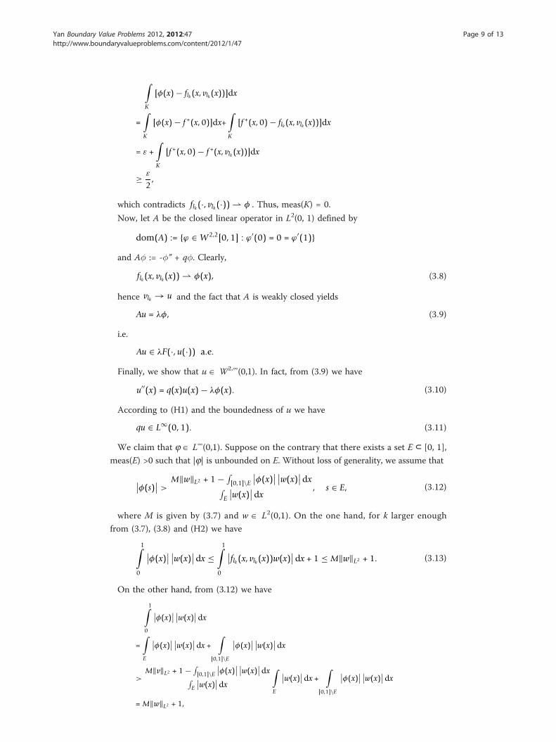
∫K

[φ(x) − flk(x, vlk(x))]dx

=∫K

[φ(x) − f +(x, 0)]dx+∫K

[f +(x, 0) − flk(x, vlk(x))]dx

= ε +∫K

[f +(x, 0) − f +(x, vlk(x))]dx

≥ ε

2,

which contradicts flk(·, vlk(·)) ⇀ φ . Thus, meas(K) = 0.

Now, let A be the closed linear operator in L2(0, 1) defined by

dom(A) := {ϕ ∈ W2,2[0, 1] : ϕ′(0) = 0 = ϕ′(1)}and A� := -�” + q�. Clearly,

flk(x, vlk(x)) ⇀ φ(x), (3:8)

hence vlk → u and the fact that A is weakly closed yields

Au = λφ, (3:9)

i.e.

Au ∈ λF(·, u(·)) a.e.

Finally, we show that u Î W2,∞(0,1). In fact, from (3.9) we have

u′′(x) = q(x)u(x) − λφ(x). (3:10)

According to (H1) and the boundedness of u we have

qu ∈ L∞(0, 1). (3:11)

We claim that j Î L∞(0,1). Suppose on the contrary that there exists a set E ⊂ [0, 1],

meas(E) >0 such that |j| is unbounded on E. Without loss of generality, we assume that

∣∣φ(s)∣∣ >M‖w‖L2 + 1 − ∫

[0,1]\E∣∣φ(x)∣∣ ∣∣w(x)∣∣dx∫

E

∣∣w(x)∣∣dx , s ∈ E, (3:12)

where M is given by (3.7) and w Î L2(0,1). On the one hand, for k larger enough

from (3.7), (3.8) and (H2) we have

1∫0

∣∣φ(x)∣∣ ∣∣w(x)∣∣dx ≤1∫

0

∣∣flk(x, vlk(x))w(x)∣∣dx + 1 ≤ M‖w‖L2 + 1. (3:13)

On the other hand, from (3.12) we have

1∫0

∣∣φ(x)∣∣ ∣∣w(x)∣∣dx=

∫E

∣∣φ(x)∣∣ ∣∣w(x)∣∣dx + ∫[0,1]\E

∣∣φ(x)∣∣ ∣∣w(x)∣∣dx

>M‖v‖L2 + 1 − ∫

[0,1]\E∣∣φ(x)∣∣ ∣∣w(x)∣∣dx∫

E

∣∣w(x)∣∣dx∫E

∣∣w(x)∣∣dx + ∫[0,1]\E

∣∣φ(x)∣∣ ∣∣w(x)∣∣dx= M‖w‖L2 + 1,


of 13

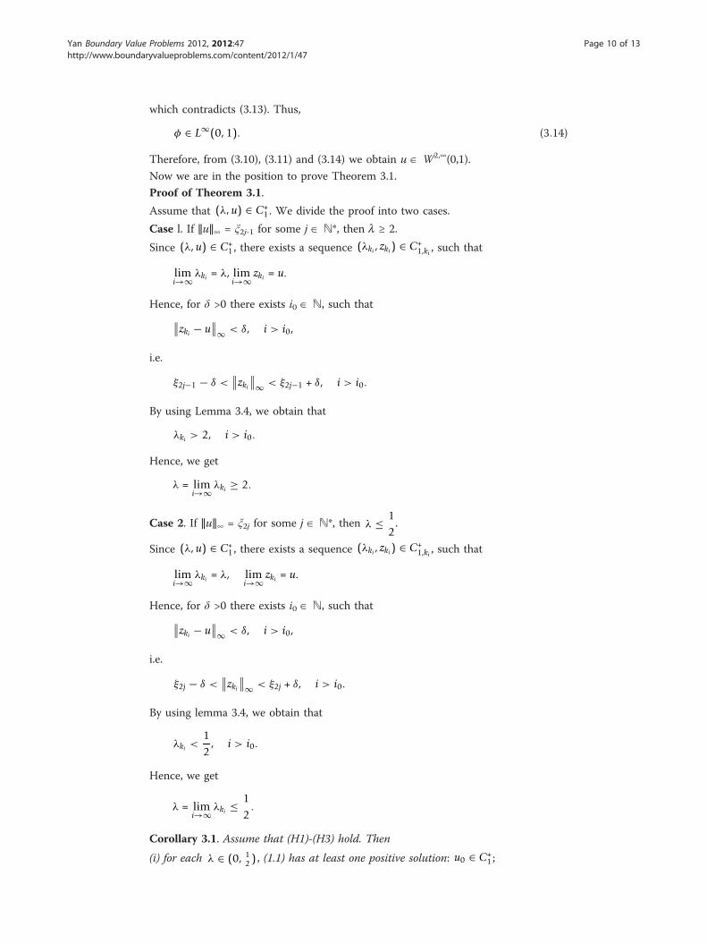
which contradicts (3.13). Thus,

φ ∈ L∞(0, 1). (3:14)

Therefore, from (3.10), (3.11) and (3.14) we obtain u Î W2,∞(0,1).

Now we are in the position to prove Theorem 3.1.

Proof of Theorem 3.1.

Assume that (λ, u) ∈ C+1 . We divide the proof into two cases.

Case l. If ∥u∥∞ = ξ2j-1 for some j Î N*, then l ≥ 2.

Since (λ, u) ∈ C+1 , there exists a sequence (λki , zki) ∈ C+

1,ki , such that

limi→∞

λki = λ, limi→∞

zki = u.

Hence, for δ >0 there exists i0 Î N, such that∥∥zki − u∥∥

∞ < δ, i > i0,

i.e.

ξ2j−1 − δ <∥∥zki∥∥∞ < ξ2j−1 + δ, i > i0.

By using Lemma 3.4, we obtain that

λki > 2, i > i0.

Hence, we get

λ = limi→∞

λki ≥ 2.

Case 2. If ∥u∥∞ = ξ2j for some j Î N*, then λ ≤ 12.

Since (λ, u) ∈ C+1 , there exists a sequence (λki , zki) ∈ C+

1,ki , such that

limi→∞

λki = λ, limi→∞

zki = u.

Hence, for δ >0 there exists i0 Î N, such that∥∥zki − u∥∥

∞ < δ, i > i0,

i.e.

ξ2j − δ <∥∥zki∥∥∞ < ξ2j + δ, i > i0.

By using lemma 3.4, we obtain that

λki <12, i > i0.

Hence, we get

λ = limi→∞

λki ≤ 12.

Corollary 3.1. Assume that (H1)-(H3) hold. Then

(i) for each λ ∈ (0, 12 ) , (1.1) has at least one positive solution: u0 ∈ C+1 ;


of 13

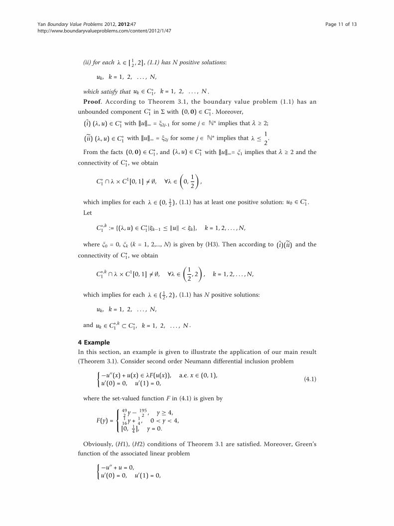
(ii) for each λ ∈ [ 12 , 2], (1.1) has N positive solutions:

uk, k = 1, 2, . . . , N,

which satisfy that uk ∈ C+1, k = 1, 2, . . . , N .

Proof. According to Theorem 3.1, the boundary value problem (1.1) has an

unbounded component C+1 in Σ with (0,0) ∈ C+

1 . Moreover,

(i) (λ, u) ∈ C+1 with ∥u∥∞ = ξ2j-1 for some j Î N* implies that l ≥ 2;

(ii) (λ, u) ∈ C+1 with ∥u∥∞ = ξ2j for some j Î N* implies that λ ≤ 1

2.

From the facts (0,0) ∈ C+1 , and (λ, u) ∈ C+

1 with ∥u∥∞= ξ1 implies that l ≥ 2 and the

connectivity of C+1 , we obtain

C+1 ∩ λ × C1[0, 1] �= ∅, ∀λ ∈

(0,

12

),

which implies for each λ ∈ (0, 12 ) , (1.1) has at least one positive solution: u0 ∈ C+1 .

Let

C+,k1 := {(λ, u) ∈ C+

1|ξk−1 ≤ ‖u‖ < ξk}, k = 1, 2, . . . ,N,

where ξ0 = 0, ξk (k = 1, 2,..., N) is given by (H3). Then according to (i)(ii) and the

connectivity of C+1 , we obtain

C+,k1 ∩ λ × C1[0, 1] �= ∅, ∀λ ∈

(12, 2

), k = 1, 2, . . . ,N,

which implies for each λ ∈ ( 12 , 2) , (1.1) has N positive solutions:

uk, k = 1, 2, . . . , N,

and uk ∈ C+,k1 ⊂ C+

1, k = 1, 2, . . . , N .

4 ExampleIn this section, an example is given to illustrate the application of our main result

(Theorem 3.1). Consider second order Neumann differential inclusion problem{−u′′(x) + u(x) ∈ λF(u(x)), a.e. x ∈ (0, 1),u′(0) = 0, u′(1) = 0,

(4:1)

where the set-valued function F in (4.1) is given by

F(y) =

⎧⎨⎩

492 y − 195

2 , y ≥ 4,116y +

14 , 0 < y < 4,

[0, 14 ], y = 0.

Obviously, (H1), (H2) conditions of Theorem 3.1 are satisfied. Moreover, Green’s

function of the associated linear problem{−u′′ + u = 0,u′(0) = 0, u′(1) = 0,


of 13

can be explicitly expressed by

G(x, s) =1

2(e − e−1)

{(ex−1 + e1−x)(es + e−s), 0 ≤ s ≤ x ≤ 1,(ex + e−x)(es−1 + e1−s), 0 ≤ x ≤ s ≤ 1.

By calculation we can get∫ 10 G(s, s)ds = e

e−e−1 ,∫ 10 G

( 12 , s

)ds = 1 and σ = 2

e+e−1 .

Let ξ1 = 3, ξ2 = 11, δ = 1, then we can check that ξ1 = 3 <5 < s(ξ2- δ), and

�(ξ1) =12

<34

< 1 − e−2 =12

⎛⎝ 1∫

0

G(s, s)ds

⎞⎠

−1

(ξ1 − δ),

(ξ2) ≥ 25 > 24 = 2

⎛⎝ 1∫

0

G(12, s

)ds

⎞⎠

−1

(ξ2 + δ).

So that (H3) condition of Theorem 3.1 is satisfied. Therefore, according to Theorem

3.1 the differential inclusion problem (4.1) has an unbounded component C+1 in Σ with

(0,0) ∈ C+1 . Moreover,

(i) (λ, u) ∈ C+1 with ∥u∥∞ = 3 implies that l ≥ 2;

(ii) (λ, u) ∈ C+1 with ∥u∥∞ = 11 implies that λ ≤ 1

2.

AcknowledgementsThe authors express their gratitude to Professors Ma Tian and Ma Ruyun for their guidance and encouragement, alsoto an anonymous referee for a number of valuable comments and suggestions.

Competing interestsThe authors declare that they have no competing interests.

Received: 14 October 2011 Accepted: 23 April 2012 Published: 23 April 2012

References1. Aubin, JP, Cellina, A: Differential Inclusion, vol. 264. Grundlehren Math Wiss. Springer-Verlag, Berlin (1984)2. Kunze, M: Nonsmooth dynamical systems. Lecture Notes in Mathematics, vol. 1744. Springer-Verlag, Berlin (2000)3. Clarke, FH, Ldeyaev, YS, Stern, RJ, Wolenski, PR: Nonsmooth Analysis and Control Theory. Springer-Verlag, New York

(1998)4. Clarke, FH: Optimization and Nonsmooth Analysis. SIAM, Philadelphia (1990)5. Leine, RI, Nijjmeijer, H: Dynamics and bifurcation of nonsmooth mechanical systems. Lecture Notes in Applied and

Computational Mechanics, vol. 18. Springer-Verlag, Berlin (2004)6. Gasiésdi, L, Papageorgion, NS: Nonsmooth Critical Point Theory and Nonlinear Boundary Value Problems. Chapman and

Hall/CRC, Boca Raton (2005)7. Deimling, K: Multivalued Differential Equation. Springer-Verlag, Berlin (1985)8. Kowalczyk, P, Piiroinen, PT: Two-parameter sliding bifurcation of periodic solutions in a dry-friction oscillator. Physica D.

237, 1053–1073 (2008). doi:10.1016/j.physd.2007.12.0079. Deimling, K: Resonance and clulomb friction. Diff Integr Equ. 7(3):759–765 (1994)10. Ma, R: Existence of periodic solutions of a generalized friction oscillator. Nonlinear Anal Real World Appl. 11, 3316–3322

(2010). doi:10.1016/j.nonrwa.2009.11.02411. Chang, KC: Variational methods for nondifferentable functionals and their applications to partial differential equations. J

Math Anal Appl. 80, 102–112 (1981). doi:10.1016/0022-247X(81)90095-012. Kourogenis, NC, Papageorgiou, NS: Nonsmooth critical point theory and nonlinear elliptic equation at resonance. Kodai

Math J. 23, 128–135 (2000)13. Zykov, PS: On two-point boundary value problems for second-order differential inclusions on manifolds. Appl Anal.

88(6):895–902 (2009). doi:10.1080/0003681090304223214. Hannelore, L, Csaba, V: Multiple solutions for a differential inclusion problem with nonhomogeneous boundary

conditions. Numer Funct Anal Optim. 30(5-6):566–581 (2009). doi:10.1080/0163056090298785715. Ntouyas, SK, O’ Regan, D: Existence results for semilinear neutral differential inclusions with nonlocal conditions. Diff

Equ Appl. 1(1):41–65 (2009)16. Papageorgion, NS, Staicu, V: The method of upper-lower solutions for nonlinear second order differential inclusions.

Nonlinear Anal. 67(3):708–726 (2007). doi:10.1016/j.na.2006.06.023


of 13

17. Kyritsi, S, Matzakos, N, Papageorgion, NS: Periodic problems for strongly nonlinear second-order differential inclusions. JDiff Equ. 183, 279–302 (1982)

18. Dhage, BC, Ntouyas, SK, Cho, YJ: On the second order discontinuous differential inclusions. J Appl Funt Anal.1(4):469–476 (2006)

19. Benchchra, M, Graef, JR, Ouahab, A: Oscillatory and nonoscillatory solutions of multivalued differential inclusions.Comput Math Appl. 49(9-10):1347–1354 (2005). doi:10.1016/j.camwa.2004.12.007

20. Budyko, MI: The effect of solar radiation variations on the climate of the earth. Tellus. 21, 611–619 (1969). doi:10.1111/j.2153-3490.1969.tb00466.x

21. Diaz, JI: Mathematical Analysis of Some Diffusive Energy Balance Models. Math Climate Environ. Mason, Paris (1993)22. Diaz, JI: The Mathematics of Models for Climatology and Environment, NATO ASI Series I: Global Environmental

Changes, vol. 48. Springer-Verlag, New York (1997)23. Diaz, JI, Hernandez, J, Tello, L: On the multiplicity of equilibrium solutions to a nonlinear diffusion equation on a

manifold arising in climatology. J Math Anal Appl. 216, 593–613 (1997). doi:10.1006/jmaa.1997.569124. Henderson-Sellers, A, McGuffie, KA: A Climate Modeling Primer. Wiley, Chich-ester (1987)25. Hetzer, G: A bifurcation result for Sturm-Liouville problem with a set-valued term. Mississippi State University (1997) In

Proceedings of the Third Mississippi State Conference on Difference Equations and Computational Simulations: 16-17May 1997

26. Jiang, D, Liu, H: Existence of positive solutions to second order Neumann boundary value problem. J Math Res Expo.20, 360–364 (2000)

27. Chu, JF, Sun, YG, Chen, H: Positive solutions of Neumann problems with singularities. J Math Anal Appl. 337, 1267–1272(2008). doi:10.1016/j.jmaa.2007.04.070

28. Sun, Y, Cho, YJ, O’ Regan, D: Positive solution for singular second order Neumann boundary value problems via a conefixed point theorem. Appl Math Comput. 210, 80–86 (2009). doi:10.1016/j.amc.2008.11.025

29. Whyburn, GT: Topological Analysis. Princeton University Press, Princeton, NJ (1964)30. Ma, R, An, Y: Global structure of positive solutions for nonlocal boundary value problems involving integral conditions.

Nonlinear Anal TMA. 71(10):4364–4376 (2009). doi:10.1016/j.na.2009.02.11331. Kuratowski, C: Topologie II. Warszawa (1950)32. Zeidler, E: Nonlinear Functional Analysis and its Applications I (Fixed-point theorems). Springer-Verlag, New York (1986)33. Mavinga, N, Nkashama, MN: Steklov-Neumann eigenproblems and nonlinear elliptic equations with nonlinear boundary

conditions. J Diff Equ. 248, 1212–1229 (2010). doi:10.1016/j.jde.2009.10.005

doi:10.1186/1687-2770-2012-47Cite this article as: Yan: Oscillating global continua of positive solutions of second order Neumann problemwith a set-valued term. Boundary Value Problems 2012 2012:47.

Submit your manuscript to a journal and benefi t from:

7 Convenient online submission

7 Rigorous peer review

7 Immediate publication on acceptance

7 Open access: articles freely available online

7 High visibility within the fi eld

7 Retaining the copyright to your article

Submit your next manuscript at 7 springeropen.com


of 13

http://www.springeropen.com/

http://www.springeropen.com/

CORPUS AND TEXT PROCESSING FOR LANGUAGE TEACHING : ON-LINE

Documents

Transcript of CORPUS AND TEXT PROCESSING FOR LANGUAGE TEACHING : ON-LINE