Copyright © 2010, 2007, 2004 Pearson Education, Inc. 8.1 - 1 Chapter 8 Hypothesis Testing 8-1...
144
Copyright © 2010, 2007, 2004 Pearson Education, Inc. 8.1 - 1 Chapter 8 Hypothesis Testing 8-1 Review and Preview 8-2 Basics of Hypothesis Testing 8-3 Testing a Claim about a Proportion 8-4 Testing a Claim About a Mean: σ Known 8-5 Testing a Claim About a Mean: σ Not Known 8-6 Testing a Claim About a Standard Deviation or Variance
-
Upload
olivia-gibson -
Category
Documents
-
view
220 -
download
0
Transcript of Copyright © 2010, 2007, 2004 Pearson Education, Inc. 8.1 - 1 Chapter 8 Hypothesis Testing 8-1...
Copyright © 2010, 2007, 2004 Pearson Education, Inc. 8.1 - 1
Chapter 8Hypothesis Testing
8-1 Review and Preview
8-2 Basics of Hypothesis Testing
8-3 Testing a Claim about a Proportion
8-4 Testing a Claim About a Mean: σ Known
8-5 Testing a Claim About a Mean: σ Not Known
8-6 Testing a Claim About a Standard Deviation or Variance

Copyright © 2010, 2007, 2004 Pearson Education, Inc. 8.1 - 2
Section 8-1Review and Preview
Copyright © 2010, 2007, 2004 Pearson Education, Inc. 8.1 - 3
ReviewIn Chapters 2 and 3 we used “descriptive statistics” when we summarized data using tools such as graphs, and statistics such as the mean and standard deviation. Methods of inferential statistics use sample data to make an inference or conclusion about a population. The two main activities of inferential statistics are using sample data to (1) estimate a population parameter (such as estimating a population parameter with a confidence interval), and (2) test a hypothesis or claim about a population parameter. In Chapter 7 we presented methods for estimating a population parameter with a confidence interval, and in this chapter we present the method of hypothesis testing.
Copyright © 2010, 2007, 2004 Pearson Education, Inc. 8.1 - 4
Definitions
In statistics, a hypothesis is a claim or statement about a property of a population.
A hypothesis test (or test of significance) is a standard procedure for testing a claim about a property of a population.
Copyright © 2010, 2007, 2004 Pearson Education, Inc. 8.1 - 5
Main Objective
The main objective of this chapter is to develop the ability to conduct hypothesis tests for claims made about a population proportion p, a population mean , or a population standard deviation .
Copyright © 2010, 2007, 2004 Pearson Education, Inc. 8.1 - 6
Examples of Hypotheses that can be Tested
• Genetics: The Genetics & IVF Institute claims that its XSORT method allows couples to increase the probability of having a baby girl.
• Business: A newspaper headline makes the claim that most workers get their jobs through networking.
• Medicine: Medical researchers claim that when people with colds are treated with echinacea, the treatment has no effect.
Copyright © 2010, 2007, 2004 Pearson Education, Inc. 8.1 - 7
Examples of Hypotheses that can be Tested
• Aircraft Safety: The Federal Aviation Administration claims that the mean weight of an airline passenger (including carry-on baggage) is greater than 185 lb, which it was 20 years ago.
• Quality Control: When new equipment is used to manufacture aircraft altimeters, the new altimeters are better because the variation in the errors is reduced so that the readings are more consistent. (In many industries, the quality of goods and services can often be improved by reducing variation.)
Copyright © 2010, 2007, 2004 Pearson Education, Inc. 8.1 - 8
Caution
When conducting hypothesis tests as described in this chapter and the following chapters, instead of jumping directly to procedures and calculations, be sure to consider the context of the data, the source of the data, and the sampling method used to obtain the sample data.

Copyright © 2010, 2007, 2004 Pearson Education, Inc. 8.1 - 9
Section 8-2 Basics of Hypothesis
Testing

Copyright © 2010, 2007, 2004 Pearson Education, Inc. 8.1 - 10
Key Concept
This section presents individual components of a hypothesis test. We should know and understand the following:• How to identify the null hypothesis and alternative
hypothesis from a given claim, and how to express both in symbolic form
• How to calculate the value of the test statistic, given a claim and sample data
• How to identify the critical value(s), given a significance level
• How to identify the P-value, given a value of the test statistic
• How to state the conclusion about a claim in simple and nontechnical terms
Copyright © 2010, 2007, 2004 Pearson Education, Inc. 8.1 - 11
Part 1:
The Basics of Hypothesis Testing
Copyright © 2010, 2007, 2004 Pearson Education, Inc. 8.1 - 12
Rare Event Rule for Inferential Statistics
If, under a given assumption, the probability of a particular observed event is exceptionally small, we conclude that the assumption is probably not correct.
Copyright © 2010, 2007, 2004 Pearson Education, Inc. 8.1 - 13
Components of aFormal Hypothesis
Test
Copyright © 2010, 2007, 2004 Pearson Education, Inc. 8.1 - 14
Null Hypothesis: H0
• The null hypothesis (denoted by H0) is a statement that the value of a population parameter (such as proportion, mean, or standard deviation) is equal to some claimed value.
• We test the null hypothesis directly.
• Either reject H0 or fail to reject H0.
Copyright © 2010, 2007, 2004 Pearson Education, Inc. 8.1 - 15
Alternative Hypothesis: H1
• The alternative hypothesis (denoted by H1 or Ha or HA) is the statement that the parameter has a value that somehow differs from the null hypothesis.
• The symbolic form of the alternative hypothesis must use one of these symbols: , <, >.
Copyright © 2010, 2007, 2004 Pearson Education, Inc. 8.1 - 16
Note about Forming Your Own Claims (Hypotheses)
If you are conducting a study and want to use a hypothesis test to support your claim, the claim must be worded so that it becomes the alternative hypothesis.
Copyright © 2010, 2007, 2004 Pearson Education, Inc. 8.1 - 17
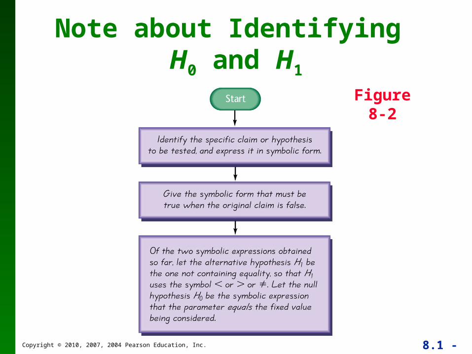
Note about Identifying H0 and H1
Figure 8-2
Copyright © 2010, 2007, 2004 Pearson Education, Inc. 8.1 - 18
Example:
Consider the claim that the mean weight of airline passengers (including carry-on baggage) is at most 195 lb (the current value used by the Federal Aviation Administration). Follow the three-step procedure outlined in Figure 8-2 to identify the null hypothesis and the alternative hypothesis.
Copyright © 2010, 2007, 2004 Pearson Education, Inc. 8.1 - 19
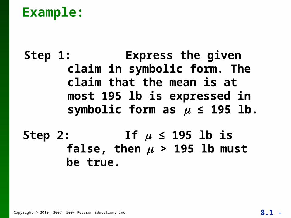
Example:
Step 1: Express the given claim in symbolic form. The claim that the mean is at most 195 lb is expressed in symbolic form as ≤ 195 lb.
Step 2: If ≤ 195 lb is false, then > 195 lb
must be true.
Copyright © 2010, 2007, 2004 Pearson Education, Inc. 8.1 - 20
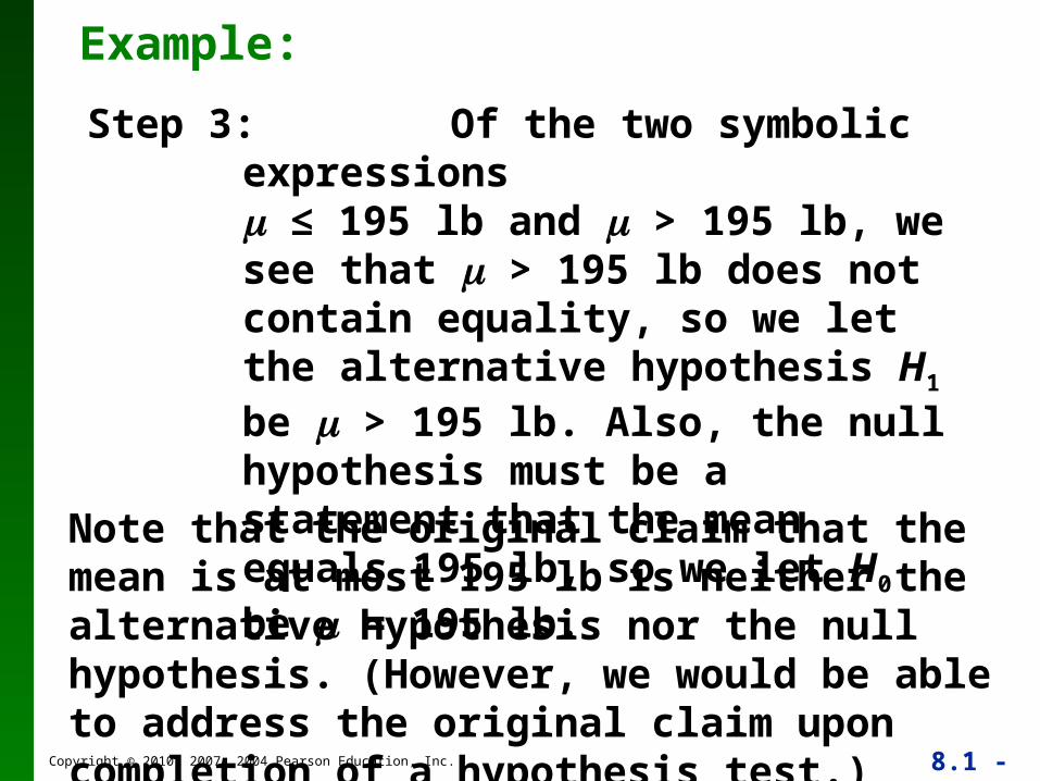
Example:
Step 3: Of the two symbolic expressions ≤ 195 lb and > 195 lb, we see that > 195 lb does not contain equality, so we let the alternative hypothesis H1 be > 195 lb. Also, the null hypothesis must be a statement that the mean equals 195 lb, so we let H0 be = 195 lb.
Note that the original claim that the mean is at most 195 lb is neither the alternative hypothesis nor the null hypothesis. (However, we would be able to address the original claim upon completion of a hypothesis test.)

Copyright © 2010, 2007, 2004 Pearson Education, Inc. 8.1 - 21
The test statistic is a value used in making a decision about the null hypothesis, and is found by converting the sample statistic to a score with the assumption that the null hypothesis is true.
Test Statistic
Copyright © 2010, 2007, 2004 Pearson Education, Inc. 8.1 - 22
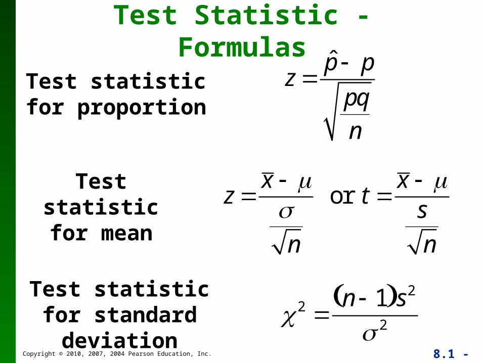
Test Statistic - Formulas
Test statistic for proportion
Test statistic for standard deviation
z p̂ p
pqn
Test statistic for mean
z x n
or t x
s
n
2 n 1 s2
2
Copyright © 2010, 2007, 2004 Pearson Education, Inc. 8.1 - 23
Example:
Let’s again consider the claim that the XSORT method of gender selection increases the likelihood of having a baby girl. Preliminary results from a test of the XSORT method of gender selection involved 14 couples who gave birth to 13 girls and 1 boy. Use the given claim and the preliminary results to calculate the value of the test statistic. Use the format of the test statistic given above, so that a normal distribution is used to approximate a binomial distribution. (There are other exact methods that do not use the normal approximation.)
Copyright © 2010, 2007, 2004 Pearson Education, Inc. 8.1 - 24
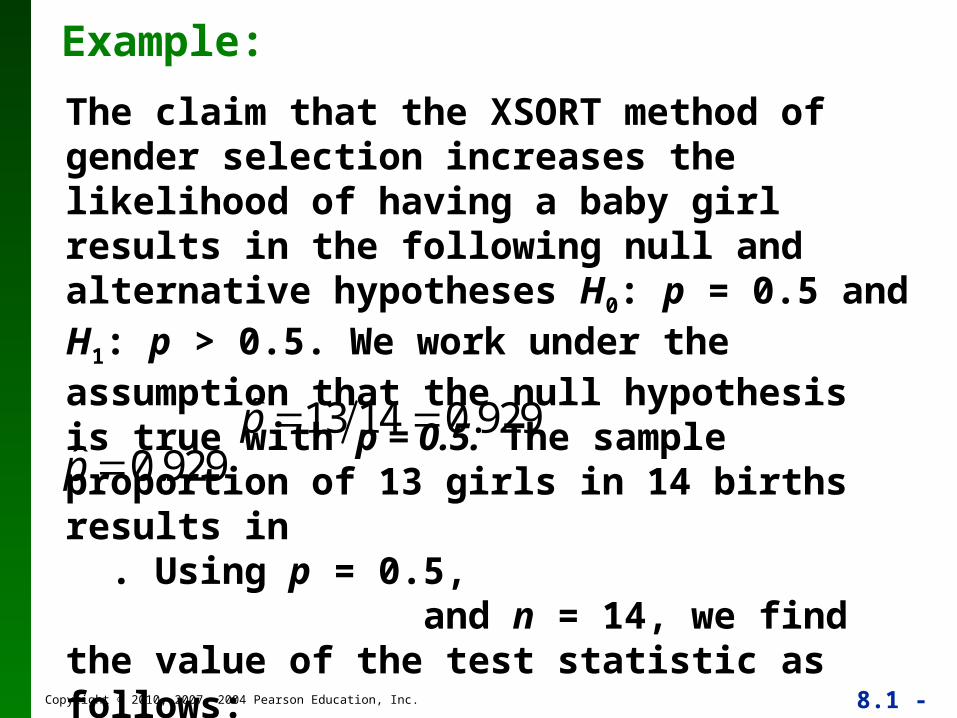
Example:
The claim that the XSORT method of gender selection increases the likelihood of having a baby girl results in the following null and alternative hypotheses H0: p = 0.5 andH1: p > 0.5. We work under the assumption that the null hypothesis is true with p = 0.5. The sample proportion of 13 girls in 14 births results in . Using p = 0.5, and n = 14, we find the value of the test statistic as follows:
p̂ 13 14 0.929p̂ 0.929
Copyright © 2010, 2007, 2004 Pearson Education, Inc. 8.1 - 25
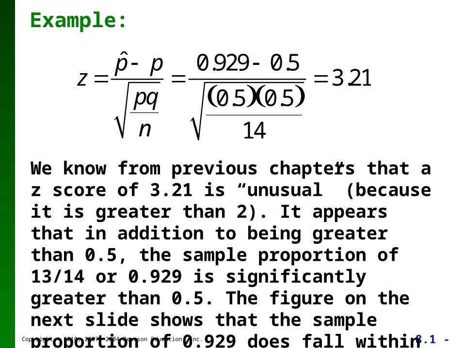
Example:
We know from previous chapters that a z score of 3.21 is “unusual” (because it is greater than 2). It appears that in addition to being greater than 0.5, the sample proportion of 13/14 or 0.929 is significantly greater than 0.5. The figure on the next slide shows that the sample proportion of 0.929 does fall within the range of values considered to be significant because
z p̂ p
pqn
0.929 0.5
0.5 0.5 14
3.21
Copyright © 2010, 2007, 2004 Pearson Education, Inc. 8.1 - 26
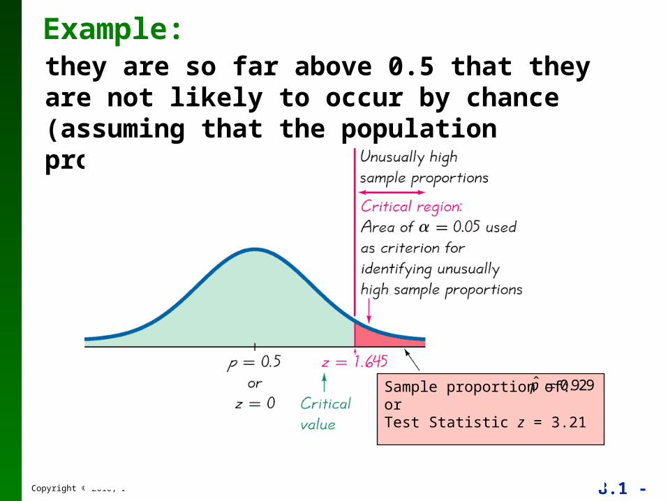
Example:they are so far above 0.5 that they are not likely to occur by chance (assuming that the population proportion is p = 0.5).
Sample proportion of: orTest Statistic z = 3.21
p̂ 0.929
Copyright © 2010, 2007, 2004 Pearson Education, Inc. 8.1 - 27
Critical Region
The critical region (or rejection region) is the set of all values of the test statistic that cause us to reject the null hypothesis. For example, see the red-shaded region in the previous figure.
Copyright © 2010, 2007, 2004 Pearson Education, Inc. 8.1 - 28
Significance Level
The significance level (denoted by ) is the probability that the test statistic will fall in the critical region when the null hypothesis is actually true. This is the same introduced in Section 7-2. Common choices for are 0.05, 0.01, and 0.10.
Copyright © 2010, 2007, 2004 Pearson Education, Inc. 8.1 - 29
Critical Value
A critical value is any value that separates the critical region (where we reject the null hypothesis) from the values of the test statistic that do not lead to rejection of the null hypothesis. The critical values depend on the nature of the null hypothesis, the sampling distribution that applies, and the significance level . See the previous figure where the critical value of z = 1.645 corresponds to a significance level of = 0.05.
Copyright © 2010, 2007, 2004 Pearson Education, Inc. 8.1 - 30
P-ValueThe P-value (or p-value or probability value) is the probability of getting a value of the test statistic that is at least as extreme as the one representing the sample data, assuming that the null hypothesis is true.
Critical region in the left tail:
Critical region in the right tail:
Critical region in two tails:
P-value = area to the left of the test statistic
P-value = area to the right of the test statistic
P-value = twice the area in the tail beyond the test statistic
Copyright © 2010, 2007, 2004 Pearson Education, Inc. 8.1 - 31
P-Value
The null hypothesis is rejected if the P-value is very small, such as 0.05 or less.
Here is a memory tool useful for interpreting the P-value:
If the P is low, the null must go.If the P is high, the null will fly.
Copyright © 2010, 2007, 2004 Pearson Education, Inc. 8.1 - 32
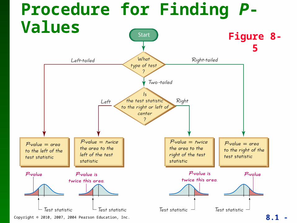
Procedure for Finding P-ValuesFigure 8-5

Copyright © 2010, 2007, 2004 Pearson Education, Inc. 8.1 - 33
Caution
Don’t confuse a P-value with a proportion p.Know this distinction:
P-value = probability of getting a test statistic at least as extreme as the one representing sample data
p = population proportion
Copyright © 2010, 2007, 2004 Pearson Education, Inc. 8.1 - 34
Example
Consider the claim that with the XSORT method of gender selection, the likelihood of having a baby girl is different from p = 0.5, and use the test statistic z = 3.21 found from 13 girls in 14 births. First determine whether the given conditions result in a critical region in the right tail, left tail, or two tails, then use Figure 8-5 to find the P-value. Interpret the P-value.
Copyright © 2010, 2007, 2004 Pearson Education, Inc. 8.1 - 35
Example
The claim that the likelihood of having a baby girl is different from p = 0.5 can be expressed as p ≠ 0.5 so the critical region is in two tails. Using Figure 8-5 to find the P-value for a two-tailed test, we see that the P-value is twice the area to the right of the test statistic z = 3.21. We refer to Table A-2 (or use technology) to find that the area to the right of z = 3.21 is 0.0007. In this case, the P-value is twice the area to the right of the test statistic, so we have:
P-value = 2 0.0007 = 0.0014
Copyright © 2010, 2007, 2004 Pearson Education, Inc. 8.1 - 36
Example
The P-value is 0.0014 (or 0.0013 if greater precision is used for the calculations). The small P-value of 0.0014 shows that there is a very small chance of getting the sample results that led to a test statistic of z = 3.21. This suggests that with the XSORT method of gender selection, the likelihood of having a baby girl is different from 0.5.
Copyright © 2010, 2007, 2004 Pearson Education, Inc. 8.1 - 37
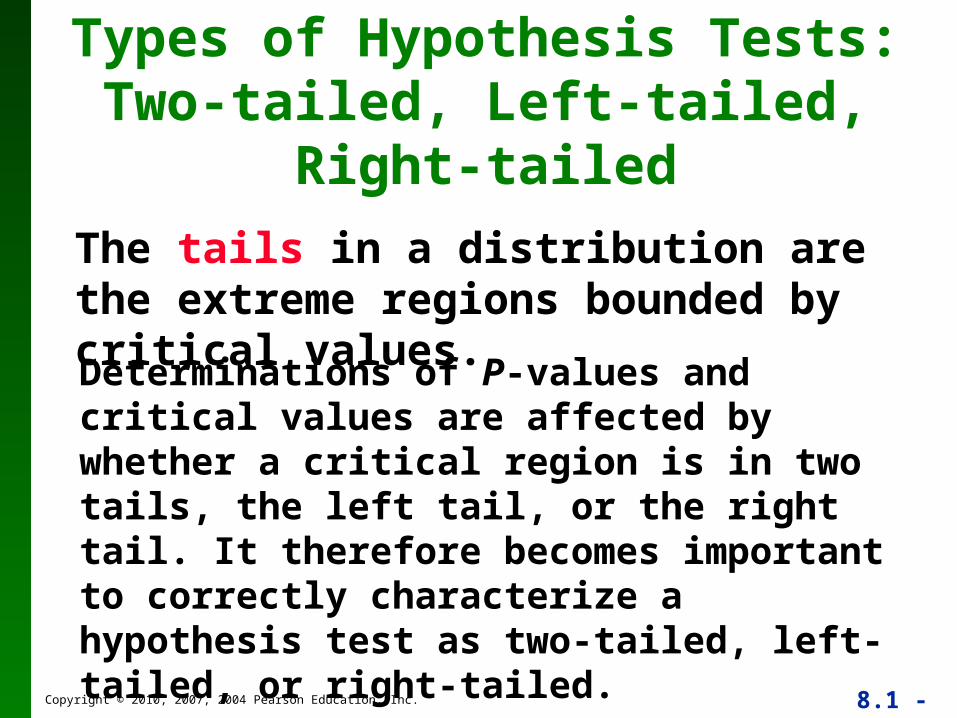
Types of Hypothesis Tests:Two-tailed, Left-tailed, Right-tailed
The tails in a distribution are the extreme regions bounded by critical values.
Determinations of P-values and critical values are affected by whether a critical region is in two tails, the left tail, or the right tail. It therefore becomes important to correctly characterize a hypothesis test as two-tailed, left-tailed, or right-tailed.
Copyright © 2010, 2007, 2004 Pearson Education, Inc. 8.1 - 38
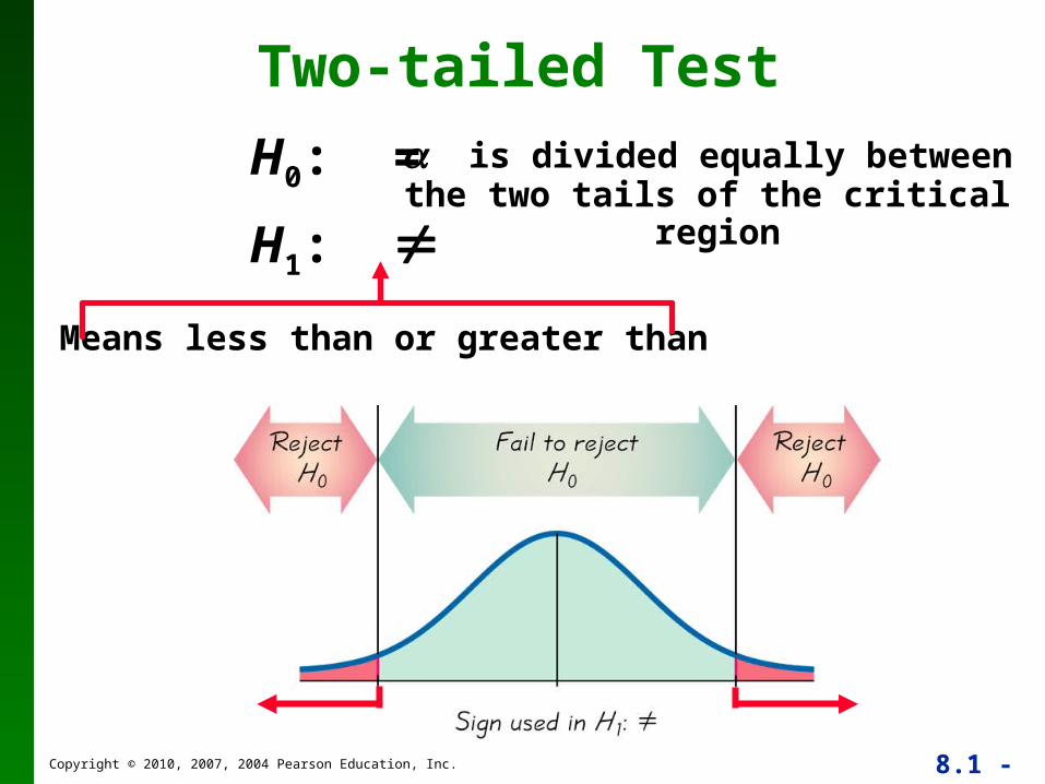
Two-tailed Test
H0: =
H1:
is divided equally between the two tails of the critical
region
Means less than or greater than
Copyright © 2010, 2007, 2004 Pearson Education, Inc. 8.1 - 39
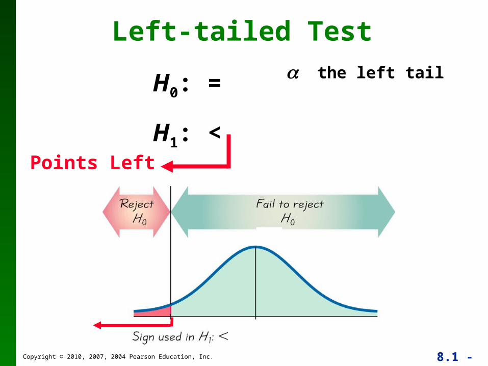
Left-tailed Test
H0: =
H1: < Points Left
the left tail
Copyright © 2010, 2007, 2004 Pearson Education, Inc. 8.1 - 40
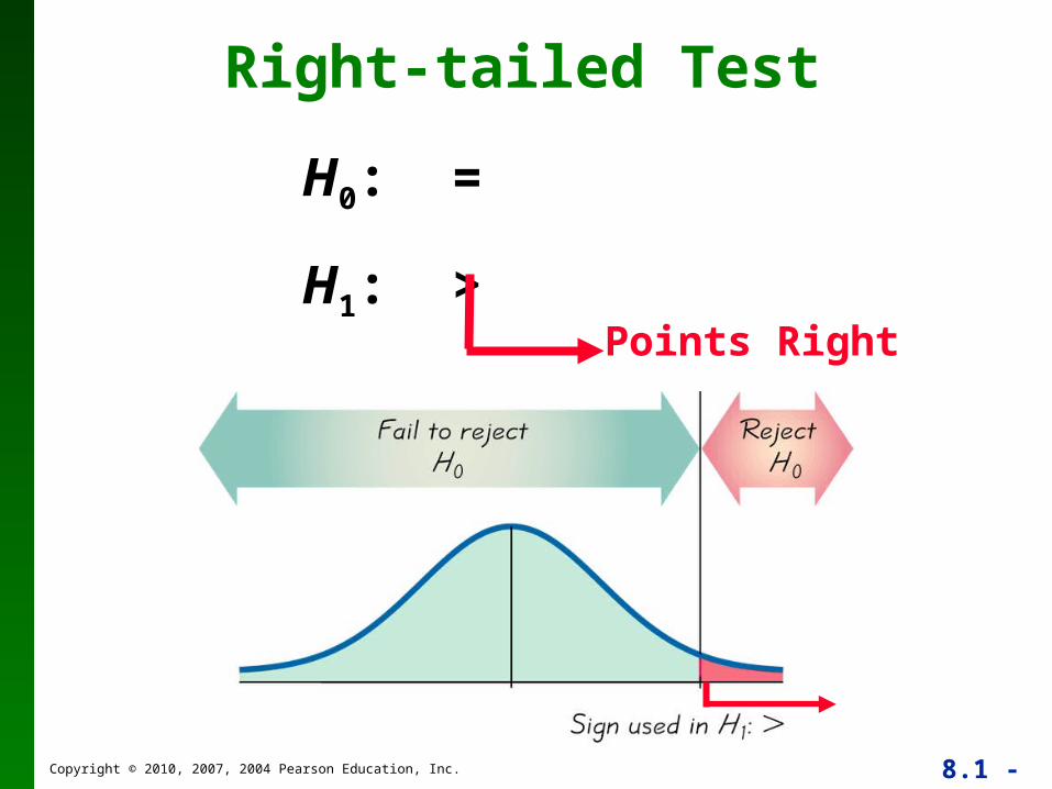
Right-tailed Test
H0: =
H1: > Points Right
Copyright © 2010, 2007, 2004 Pearson Education, Inc. 8.1 - 41
Conclusions in Hypothesis Testing
We always test the null hypothesis. The initial conclusion will always be one of the following:
1. Reject the null hypothesis.
2. Fail to reject the null hypothesis.

Copyright © 2010, 2007, 2004 Pearson Education, Inc. 8.1 - 42
P-value method:Using the significance level :
If P-value , reject H0.
If P-value > , fail to reject H0.
Decision Criterion
Copyright © 2010, 2007, 2004 Pearson Education, Inc. 8.1 - 43
Traditional method:
If the test statistic falls within the critical region, reject H0.
If the test statistic does not fall within the critical region, fail to reject H0.
Decision Criterion
Copyright © 2010, 2007, 2004 Pearson Education, Inc. 8.1 - 44
Another option:
Instead of using a significance level such as 0.05, simply identify the P-value and leave the decision to the reader.
Decision Criterion
Copyright © 2010, 2007, 2004 Pearson Education, Inc. 8.1 - 45
Decision Criterion
Confidence Intervals:
A confidence interval estimate of a population parameter contains the likely values of that parameter. If a confidence interval does not include a claimed value of a population parameter, reject that claim.
Copyright © 2010, 2007, 2004 Pearson Education, Inc. 8.1 - 46
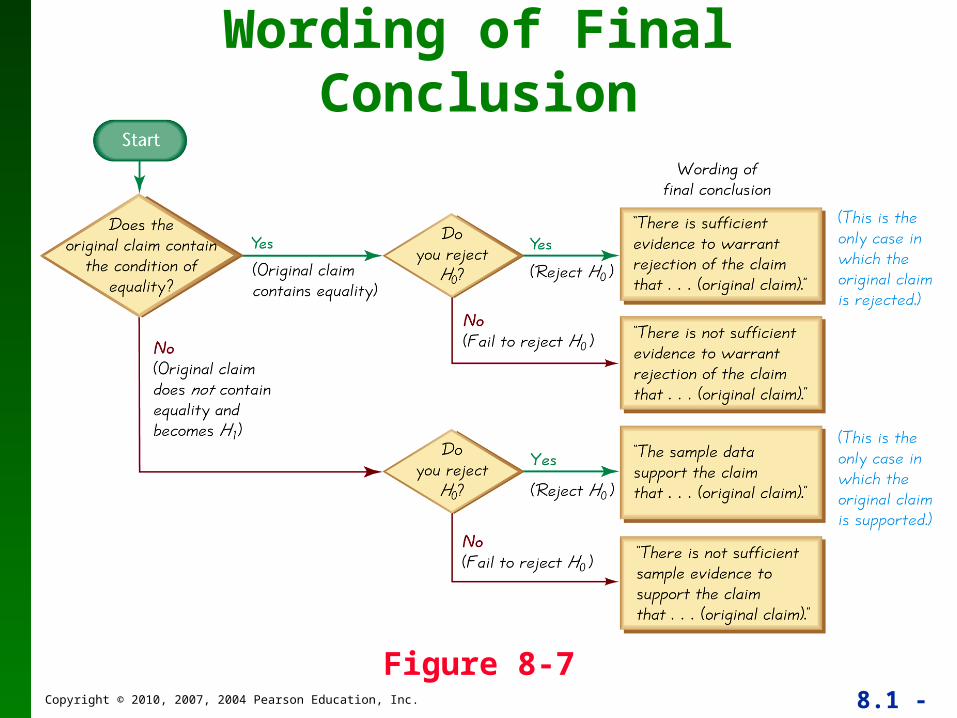
Wording of Final Conclusion
Figure 8-7
Copyright © 2010, 2007, 2004 Pearson Education, Inc. 8.1 - 47
Caution
Never conclude a hypothesis test with a statement of “reject the null hypothesis” or “fail to reject the null hypothesis.” Always make sense of the conclusion with a statement that uses simple nontechnical wording that addresses the original claim.
Copyright © 2010, 2007, 2004 Pearson Education, Inc. 8.1 - 48
Accept Versus Fail to Reject
• Some texts use “accept the null hypothesis.”
• We are not proving the null hypothesis.
• Fail to reject says more correctly
• The available evidence is not strong enough to warrant rejection of the null hypothesis (such as not enough evidence to convict a suspect).
Copyright © 2010, 2007, 2004 Pearson Education, Inc. 8.1 - 49
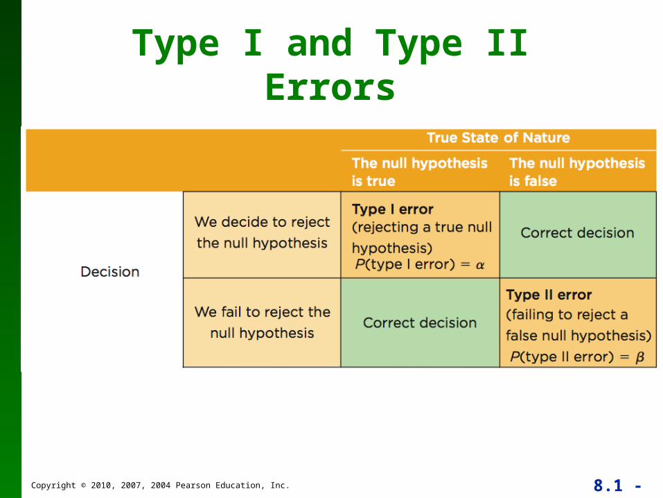
Type I Error
• A Type I error is the mistake of rejecting the null hypothesis when it is actually true.
• The symbol (alpha) is used to represent the probability of a type I error.

Copyright © 2010, 2007, 2004 Pearson Education, Inc. 8.1 - 50
Type II Error
• A Type II error is the mistake of failing to reject the null hypothesis when it is actually false.
• The symbol (beta) is used to represent the probability of a type II error.
Copyright © 2010, 2007, 2004 Pearson Education, Inc. 8.1 - 51
Type I and Type II Errors
Copyright © 2010, 2007, 2004 Pearson Education, Inc. 8.1 - 52
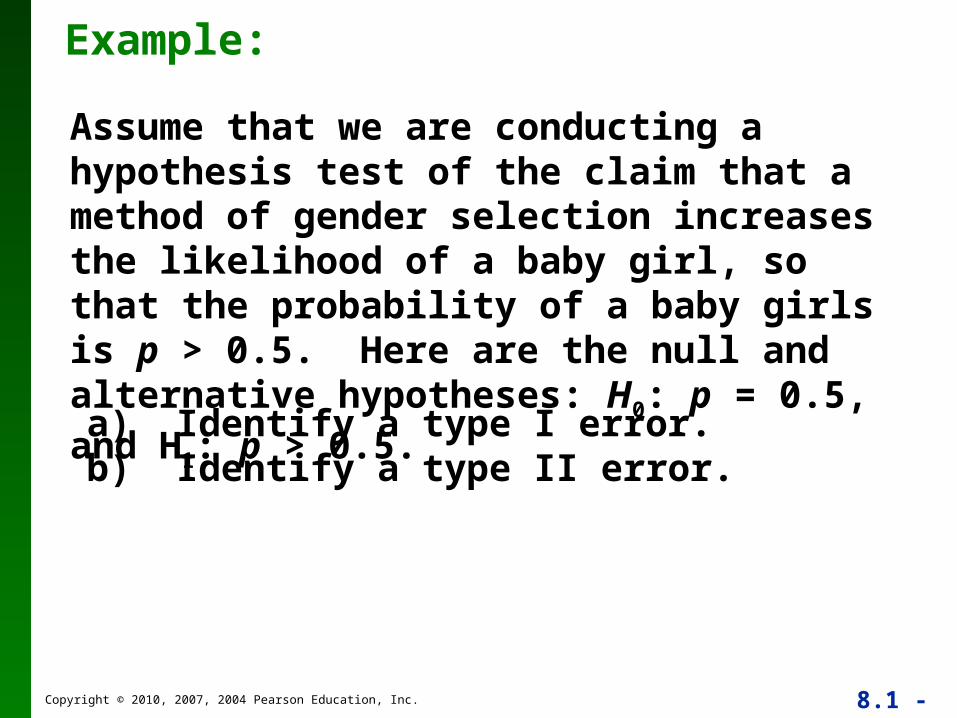
Example:
a) Identify a type I error.b) Identify a type II error.
Assume that we are conducting a hypothesis test of the claim that a method of gender selection increases the likelihood of a baby girl, so that the probability of a baby girls is p > 0.5. Here are the null and alternative hypotheses: H0: p = 0.5, and H1: p > 0.5.

Copyright © 2010, 2007, 2004 Pearson Education, Inc. 8.1 - 53
Example:
a) A type I error is the mistake of rejecting a true null hypothesis, so this is a type I error: Conclude that there is sufficient evidence to support p > 0.5, when in reality p = 0.5.
b) A type II error is the mistake of failing to reject the null hypothesis when it is false, so this is a type II error: Fail to reject p = 0.5 (and therefore fail to support p > 0.5) when in reality p > 0.5.
Copyright © 2010, 2007, 2004 Pearson Education, Inc. 8.1 - 54
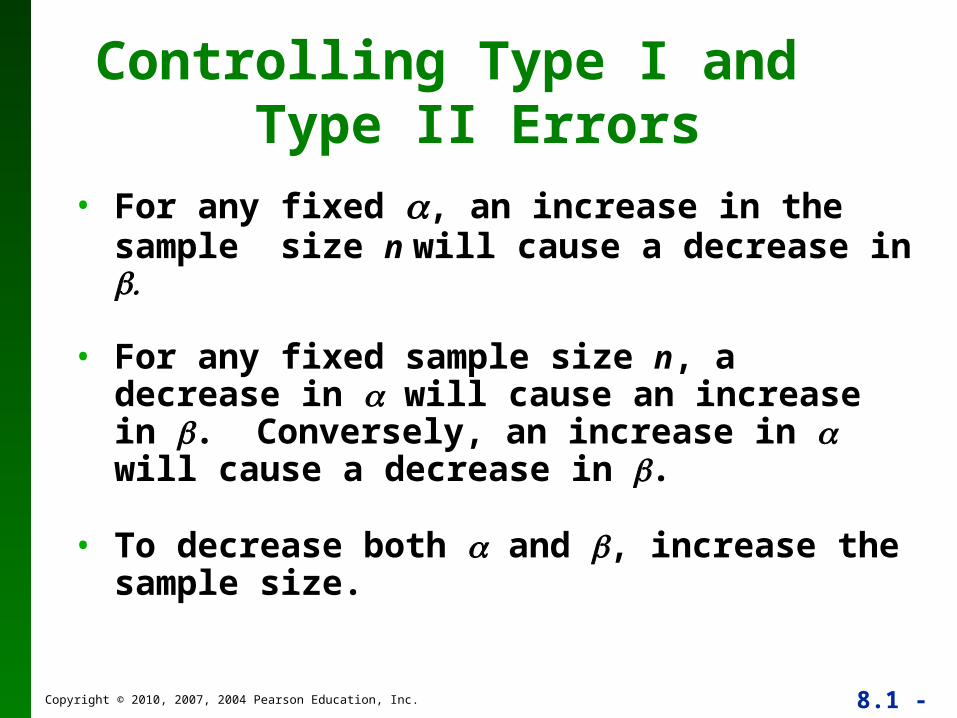
Controlling Type I and Type II Errors
• For any fixed , an increase in the sample size n will cause a decrease in
• For any fixed sample size n, a decrease in will cause an increase in . Conversely, an increase in will cause a decrease in .
• To decrease both and , increase the sample size.
Copyright © 2010, 2007, 2004 Pearson Education, Inc. 8.1 - 55
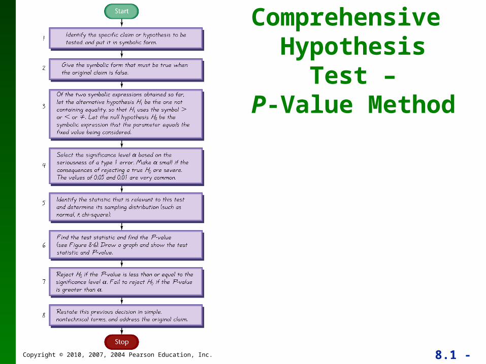
Comprehensive Hypothesis Test –P-Value Method
Copyright © 2010, 2007, 2004 Pearson Education, Inc. 8.1 - 56
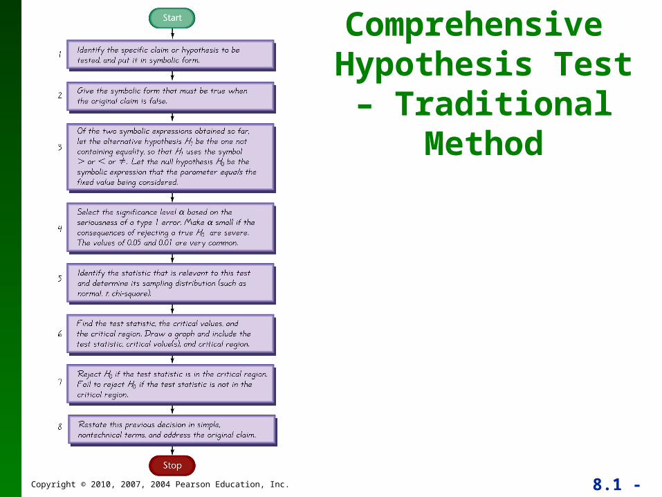
Comprehensive Hypothesis Test – Traditional Method
Copyright © 2010, 2007, 2004 Pearson Education, Inc. 8.1 - 57
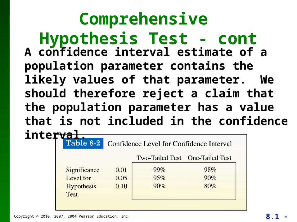
Comprehensive Hypothesis Test - cont
A confidence interval estimate of a population parameter contains the likely values of that parameter. We should therefore reject a claim that the population parameter has a value that is not included in the confidence interval.
Copyright © 2010, 2007, 2004 Pearson Education, Inc. 8.1 - 58
In some cases, a conclusion based on a confidence interval may be different from a conclusion based on a hypothesis test. See the comments in the individual sections.
Caution

Copyright © 2010, 2007, 2004 Pearson Education, Inc. 8.1 - 59
Part 2:
Beyond the Basics of Hypothesis Testing:
The Power of a Test
Copyright © 2010, 2007, 2004 Pearson Education, Inc. 8.1 - 60
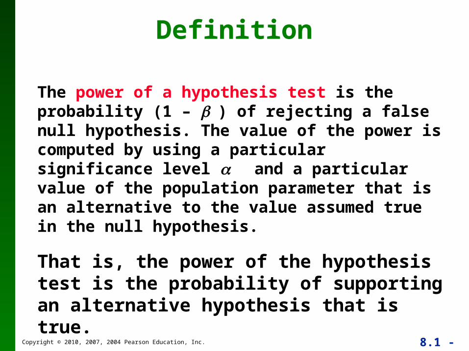
Definition
The power of a hypothesis test is the probability (1 – ) of rejecting a false null hypothesis. The value of the power is computed by using a particular significance level and a particular value of the population parameter that is an alternative to the value assumed true in the null hypothesis.
That is, the power of the hypothesis test is the probability of supporting an alternative hypothesis that is true.

Copyright © 2010, 2007, 2004 Pearson Education, Inc. 8.1 - 61
Power and theDesign of Experiments
Just as 0.05 is a common choice for a significance level, a power of at least 0.80 is a common requirement for determining that a hypothesis test is effective. (Some statisticians argue that the power should be higher, such as 0.85 or 0.90.) When designing an experiment, we might consider how much of a difference between the claimed value of a parameter and its true value is an important amount of difference. When designing an experiment, a goal of having a power value of at least 0.80 can often be used to determine the minimum required sample size.
Copyright © 2010, 2007, 2004 Pearson Education, Inc. 8.1 - 62
Recap
In this section we have discussed:
Null and alternative hypotheses.
Test statistics.
Significance levels.
P-values.
Decision criteria.
Type I and II errors.
Power of a hypothesis test.
Copyright © 2010, 2007, 2004 Pearson Education, Inc. 8.1 - 63
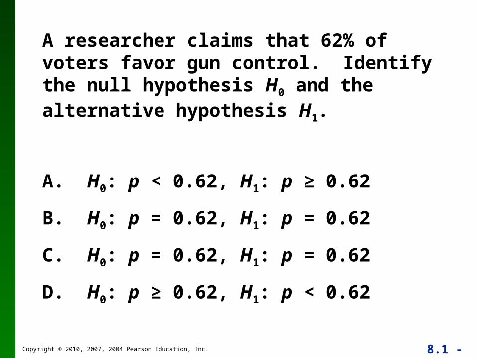
A researcher claims that 62% of voters favor gun control. Identify the null hypothesis H0 and the alternative hypothesis H1.
A. H0: p < 0.62, H1: p ≥ 0.62
B. H0: p = 0.62, H1: p = 0.62
C. H0: p = 0.62, H1: p = 0.62
D. H0: p ≥ 0.62, H1: p < 0.62
Copyright © 2010, 2007, 2004 Pearson Education, Inc. 8.1 - 64
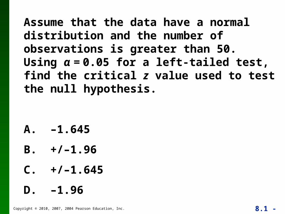
Assume that the data have a normal distribution and the number of observations is greater than 50. Using α = 0.05 for a left-tailed test, find the critical z value used to test the null hypothesis.
A. –1.645
B. +/–1.96
C. +/–1.645
D. –1.96
Copyright © 2010, 2007, 2004 Pearson Education, Inc. 8.1 - 65
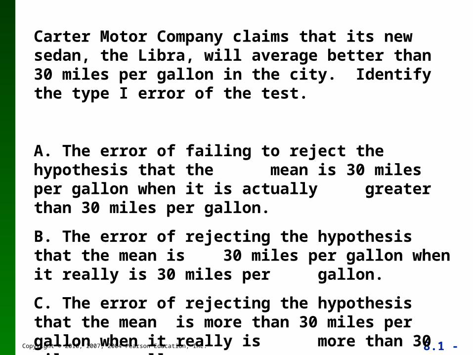
Carter Motor Company claims that its new sedan, the Libra, will average better than 30 miles per gallon in the city. Identify the type I error of the test.
A. The error of failing to reject the hypothesis that the mean is 30 miles per gallon when it is actually
greater than 30 miles per gallon.
B. The error of rejecting the hypothesis that the mean is 30 miles per gallon when it really is 30 miles per gallon.
C. The error of rejecting the hypothesis that the mean is more than 30 miles per gallon when it really is more than 30 miles per gallon.

Copyright © 2010, 2007, 2004 Pearson Education, Inc. 8.1 - 66
Section 8-3 Testing a Claim About a
Proportion
Copyright © 2010, 2007, 2004 Pearson Education, Inc. 8.1 - 67
Key Concept
This section presents complete procedures for testing a hypothesis (or claim) made about a population proportion. This section uses the components introduced in the previous section for the P-value method, the traditional method or the use of confidence intervals.
Copyright © 2010, 2007, 2004 Pearson Education, Inc. 8.1 - 68
Key Concept
Two common methods for testing a claim about a population proportion are (1) to use a normal distribution as an approximation to the binomial distribution, and (2) to use an exact method based on the binomial probability distribution. Part 1 of this section uses the approximate method with the normal distribution, and Part 2 of this section briefly describes the exact method.
Copyright © 2010, 2007, 2004 Pearson Education, Inc. 8.1 - 69
Part 1:
Basic Methods of Testing Claims about a Population Proportion p
Copyright © 2010, 2007, 2004 Pearson Education, Inc. 8.1 - 70
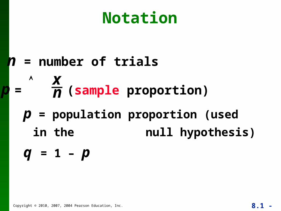
Notation
p = population proportion (used in the
null hypothesis)
q = 1 – p
n = number of trials
p = (sample proportion)xn
Copyright © 2010, 2007, 2004 Pearson Education, Inc. 8.1 - 71
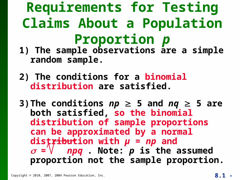
1) The sample observations are a simple random sample.
2) The conditions for a binomial distribution are satisfied.
3) The conditions np 5 and nq 5 are both satisfied, so the binomial distribution of sample proportions can be approximated by a normal distribution with µ = np and = npq . Note: p is the assumed proportion not the sample proportion.
Requirements for Testing Claims About a Population Proportion p
Copyright © 2010, 2007, 2004 Pearson Education, Inc. 8.1 - 72
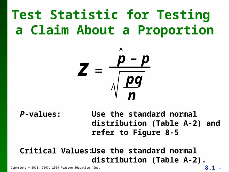
p – p
pqn
z =
Test Statistic for Testing a Claim About a Proportion
P-values:
Critical Values:
Use the standard normal distribution (Table A-2) and refer to Figure 8-5
Use the standard normal distribution (Table A-2).
Copyright © 2010, 2007, 2004 Pearson Education, Inc. 8.1 - 73
Caution
Don’t confuse a P-value with a proportion p.
P-value = probability of getting a test statistic at least as extreme as the one representing sample data
p = population proportion
Copyright © 2010, 2007, 2004 Pearson Education, Inc. 8.1 - 74
P-Value Method:
Use the same method as described in Section 8-2 and in Figure 8-8.
Use the standard normal distribution (Table A-2).
Copyright © 2010, 2007, 2004 Pearson Education, Inc. 8.1 - 75
Traditional Method
Use the same method as described in Section 8-2 and in Figure 8-9.
Copyright © 2010, 2007, 2004 Pearson Education, Inc. 8.1 - 76
Confidence Interval Method
Use the same method as described in Section 8-2 and in Table 8-2.
Copyright © 2010, 2007, 2004 Pearson Education, Inc. 8.1 - 77
CAUTION
When testing claims about a population proportion, the traditional method and the P-value method are equivalent and will yield the same result since they use the same standard deviation based on the claimed proportion p. However, the confidence interval uses an estimated standard deviation based upon the sample proportion p. Consequently, it is possible that the traditional and P-value methods may yield a different conclusion than the confidence interval method.
A good strategy is to use a confidence interval to estimate a population proportion, but use the P-value or traditional method for testing a claim about the proportion.
Copyright © 2010, 2007, 2004 Pearson Education, Inc. 8.1 - 78
Example:
The text refers to a study in which 57 out of 104 pregnant women correctly guessed the sex of their babies. Use these sample data to test the claim that the success rate of such guesses is no different from the 50% success rate expected with random chance guesses. Use a 0.05 significance level.
Copyright © 2010, 2007, 2004 Pearson Education, Inc. 8.1 - 79
Example:
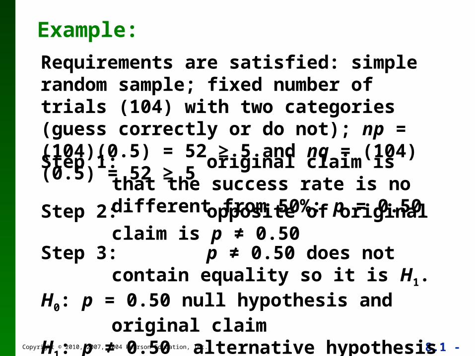
Requirements are satisfied: simple random sample; fixed number of trials (104) with two categories (guess correctly or do not); np = (104)(0.5) = 52 ≥ 5 and nq = (104)(0.5) = 52 ≥ 5
Step 1: original claim is that the success rate is no different from 50%: p = 0.50
Step 2: opposite of original claim is p ≠ 0.50
Step 3: p ≠ 0.50 does not contain equality so it is H1.
H0: p = 0.50 null hypothesis and original claimH1: p ≠ 0.50 alternative hypothesis
Copyright © 2010, 2007, 2004 Pearson Education, Inc. 8.1 - 80
Example:
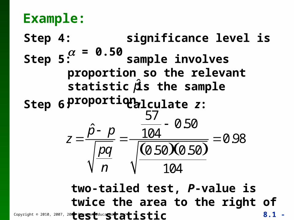
Step 4: significance level is = 0.50
Step 5: sample involves proportion so the relevant statistic is the sample proportion,
Step 6: calculate z:
p̂
z p̂ p
pqn
57104
0.50
0.50 0.50 104
0.98
two-tailed test, P-value is twice the area to the right of test statistic
Copyright © 2010, 2007, 2004 Pearson Education, Inc. 8.1 - 81
Example:
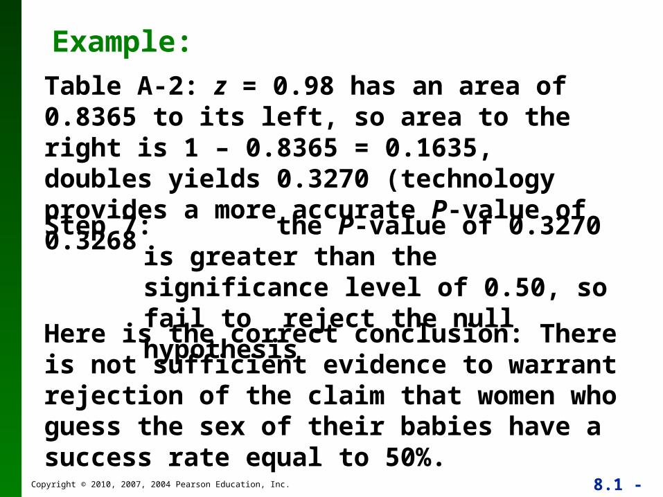
Table A-2: z = 0.98 has an area of 0.8365 to its left, so area to the right is 1 – 0.8365 = 0.1635, doubles yields 0.3270 (technology provides a more accurate P-value of 0.3268
Step 7: the P-value of 0.3270 is greater than the significance level of 0.50, so fail to reject the null hypothesis
Here is the correct conclusion: There is not sufficient evidence to warrant rejection of the claim that women who guess the sex of their babies have a success rate equal to 50%.
Copyright © 2010, 2007, 2004 Pearson Education, Inc. 8.1 - 82
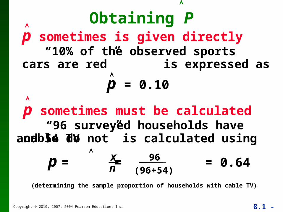
(determining the sample proportion of households with cable TV)
p = = = 0.64xn
96 (96+54)
and 54 do not” is calculated using
p sometimes must be calculated “96 surveyed households have cable TV
p sometimes is given directly “10% of the observed sports cars are red” is expressed as
p = 0.10
Obtaining P
Copyright © 2010, 2007, 2004 Pearson Education, Inc. 8.1 - 83
Part 2:
Exact Method for Testing Claims about a Proportion p
Copyright © 2010, 2007, 2004 Pearson Education, Inc. 8.1 - 84
Testing Claims
We can get exact results by using the binomial probability distribution. Binomial probabilities are a nuisance to calculate manually, but technology makes this approach quite simple. Also, this exact approach does not require that np ≥ 5 and nq ≥ 5 so we have a method that applies when that requirement is not satisfied. To test hypotheses using the exact binomial distribution, use the binomial probability distribution with the P-value method, use the value of p assumed in the null hypothesis, and find P-values as follows:

Copyright © 2010, 2007, 2004 Pearson Education, Inc. 8.1 - 85
Testing Claims
Left-tailed test:
The P-value is the probability of getting x or fewer successes among n trials.
Right-tailed test:
The P-value is the probability of getting x or more successes among n trials.
Copyright © 2010, 2007, 2004 Pearson Education, Inc. 8.1 - 86
Testing Claims
Two-tailed test:
the P-value is twice the probability of getting x or more successes
the P-value is twice the probability of getting x or fewer successes
If p̂ p,
If p̂ p,
Copyright © 2010, 2007, 2004 Pearson Education, Inc. 8.1 - 87
Recap
In this section we have discussed:
Test statistics for claims about a proportion.
P-value method.
Confidence interval method.
Obtaining p.

Copyright © 2010, 2007, 2004 Pearson Education, Inc. 8.1 - 88
Section 8-4 Testing a Claim About a
Mean: Known

Copyright © 2010, 2007, 2004 Pearson Education, Inc. 8.1 - 89
A medical school claims that more than 28% of its students plan to go into general practice. It is found that among a random sample of 130 students, 32% of them plan to go into general practice. Find the P-value for a test of the school’s claim.
A. 0.1539
B. 0.1635
C. 0.3078
D. 0.3461
Copyright © 2010, 2007, 2004 Pearson Education, Inc. 8.1 - 90
Key Concept
This section presents methods for testing a claim about a population mean, given that the population standard deviation is a known value. This section uses the normal distribution with the same components of hypothesis tests that were introduced in Section 8-2.
Copyright © 2010, 2007, 2004 Pearson Education, Inc. 8.1 - 91
Notation
n = sample size
= sample mean
= population mean of all sample means from samples of size n
= known value of the population standard deviation
x
x
Copyright © 2010, 2007, 2004 Pearson Education, Inc. 8.1 - 92
Requirements for Testing Claims About a Population Mean (with Known)
1) The sample is a simple random sample.
2) The value of the population standard deviation is known.
3) Either or both of these conditions is satisfied: The population is normally distributed or n > 30.
Copyright © 2010, 2007, 2004 Pearson Education, Inc. 8.1 - 93
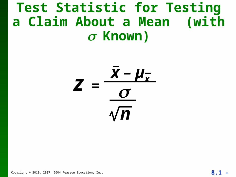
Test Statistic for Testing a Claim About a Mean (with Known)
n
x – µxz =
Copyright © 2010, 2007, 2004 Pearson Education, Inc. 8.1 - 94
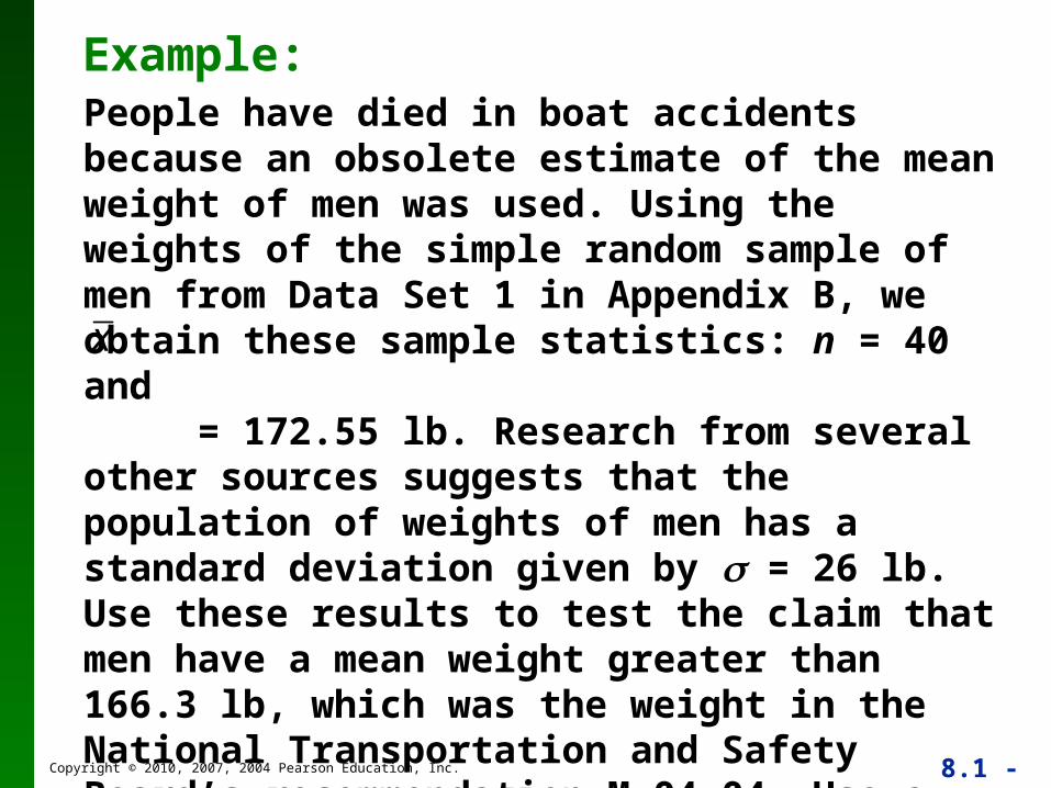
Example:People have died in boat accidents because an obsolete estimate of the mean weight of men was used. Using the weights of the simple random sample of men from Data Set 1 in Appendix B, we obtain these sample statistics: n = 40 and = 172.55 lb. Research from several other sources suggests that the population of weights of men has a standard deviation given by = 26 lb. Use these results to test the claim that men have a mean weight greater than 166.3 lb, which was the weight in the National Transportation and Safety Board’s recommendation M-04-04. Use a 0.05 significance level, and use the P-value method outlined in Figure 8-8.
x

Copyright © 2010, 2007, 2004 Pearson Education, Inc. 8.1 - 95
Example:Requirements are satisfied: simple random sample, is known (26 lb), sample size is 40 (n > 30)
Step 1: Express claim as > 166.3 lb
Step 2: alternative to claim is ≤ 166.3 lb
Step 3: > 166.3 lb does not contain equality, it is the alternative hypothesis:
H0: = 166.3 lb null hypothesisH1: > 166.3 lb alternative hypothesis and
original claim
Copyright © 2010, 2007, 2004 Pearson Education, Inc. 8.1 - 96
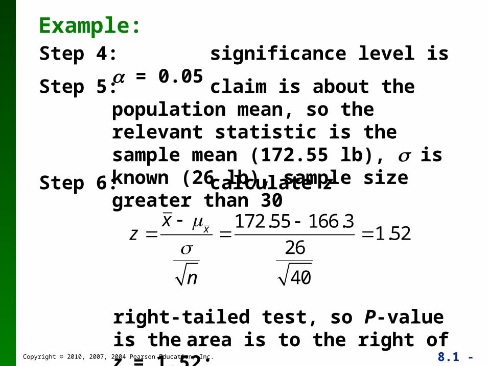
Example:Step 4: significance level is = 0.05
Step 5: claim is about the population mean, so the relevant statistic is the sample mean (172.55 lb), is known (26 lb), sample size greater than 30
Step 6: calculate z
z x
x
n
172.55 166.3
26
40
1.52
right-tailed test, so P-value is the area is to the right of z = 1.52;
Copyright © 2010, 2007, 2004 Pearson Education, Inc. 8.1 - 97
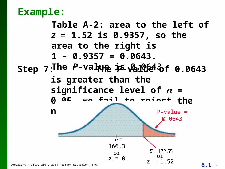
Example:Table A-2: area to the left of z = 1.52 is 0.9357, so the area to the right is1 – 0.9357 = 0.0643.The P-value is 0.0643
Step 7: The P-value of 0.0643 is greater than the significance level of = 0.05, we fail to reject the null hypothesis.
x 172.55
= 166.3or
z = 0 orz = 1.52
P-value = 0.0643
Copyright © 2010, 2007, 2004 Pearson Education, Inc. 8.1 - 98
Example:
The P-value of 0.0643 tells us that if men have a mean weight given by = 166.3 lb, there is a good chance (0.0643) of getting a sample mean of 172.55 lb. A sample mean such as 172.55 lb could easily occur by chance. There is not sufficient evidence to support a conclusion that the population mean is greater than 166.3 lb, as in the National Transportation and Safety Board’s recommendation.
Copyright © 2010, 2007, 2004 Pearson Education, Inc. 8.1 - 99
Example:
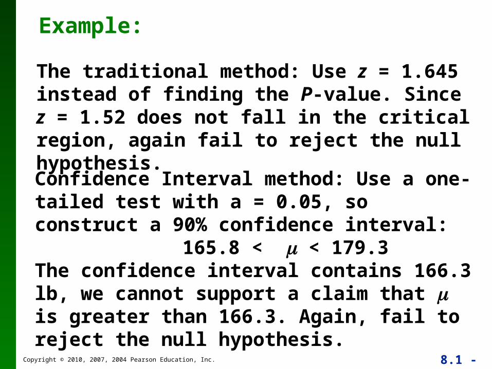
The traditional method: Use z = 1.645 instead of finding the P-value. Since z = 1.52 does not fall in the critical region, again fail to reject the null hypothesis.
Confidence Interval method: Use a one-tailed test with a = 0.05, so construct a 90% confidence interval:
165.8 < < 179.3The confidence interval contains 166.3 lb, we cannot support a claim that is greater than 166.3. Again, fail to reject the null hypothesis.
Copyright © 2010, 2007, 2004 Pearson Education, Inc. 8.1 - 100
Underlying Rationale of Hypothesis Testing
If, under a given assumption, there is an extremely small probability of getting sample results at least as extreme as the results that were obtained, we conclude that the assumption is probably not correct.
When testing a claim, we make an assumption (null hypothesis) of equality. We then compare the assumption and the sample results and we form one of the following conclusions:
Copyright © 2010, 2007, 2004 Pearson Education, Inc. 8.1 - 101
• If the sample results (or more extreme results) can easily occur when the assumption (null hypothesis) is true, we attribute the relatively small discrepancy between the assumption and the sample results to chance.
• If the sample results cannot easily occur when that assumption (null hypothesis) is true, we explain the relatively large discrepancy between the assumption and the sample results by concluding that the assumption is not true, so we reject the assumption.
Underlying Rationale of Hypotheses Testing - cont
Copyright © 2010, 2007, 2004 Pearson Education, Inc. 8.1 - 102
Recap
In this section we have discussed:
Requirements for testing claims about population means, σ known.
P-value method.
Traditional method.
Confidence interval method.
Rationale for hypothesis testing.

Copyright © 2010, 2007, 2004 Pearson Education, Inc. 8.1 - 103
Section 8-5 Testing a Claim About a
Mean: Not Known

Copyright © 2010, 2007, 2004 Pearson Education, Inc. 8.1 - 104
Key Concept
This section presents methods for testing a claim about a population mean when we do not know the value of σ. The methods of this section use the Student t distribution introduced earlier.
Copyright © 2010, 2007, 2004 Pearson Education, Inc. 8.1 - 105
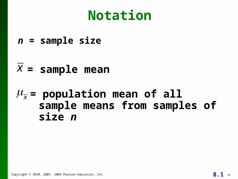
Notation
n = sample size
= sample mean
= population mean of all sample means from samples of size n
x
x
Copyright © 2010, 2007, 2004 Pearson Education, Inc. 8.1 - 106
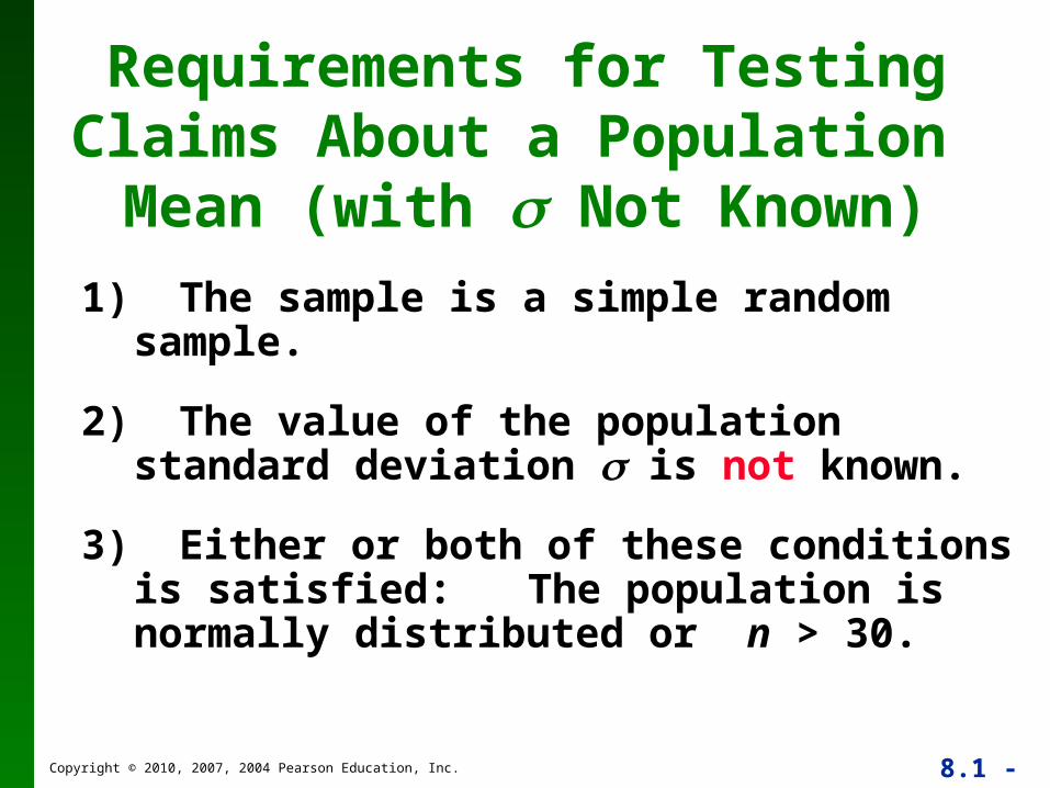
Requirements for Testing Claims About a Population
Mean (with Not Known)
1) The sample is a simple random sample.
2) The value of the population standard deviation is not known.
3) Either or both of these conditions is satisfied: The population is normally distributed or n > 30.
Copyright © 2010, 2007, 2004 Pearson Education, Inc. 8.1 - 107
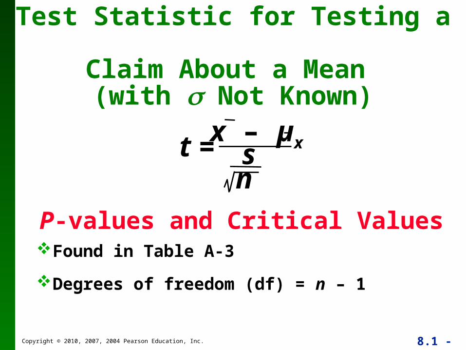
Test Statistic for Testing a Claim About a Mean (with Not Known)
P-values and Critical ValuesFound in Table A-3
Degrees of freedom (df) = n – 1
x – µxt = sn

Copyright © 2010, 2007, 2004 Pearson Education, Inc. 8.1 - 108
Important Properties of the Student t Distribution
1. The Student t distribution is different for different sample sizes (see Figure 7-5 in Section 7-4).
2. The Student t distribution has the same general bell shape as the normal distribution; its wider shape reflects the greater variability that is expected when s is used to estimate .
3. The Student t distribution has a mean of t = 0 (just as the standard normal distribution has a mean of z = 0).
4. The standard deviation of the Student t distribution varies with the sample size and is greater than 1 (unlike the standard normal distribution, which has = 1).
5. As the sample size n gets larger, the Student t distribution gets closer to the standard normal distribution.
Copyright © 2010, 2007, 2004 Pearson Education, Inc. 8.1 - 109
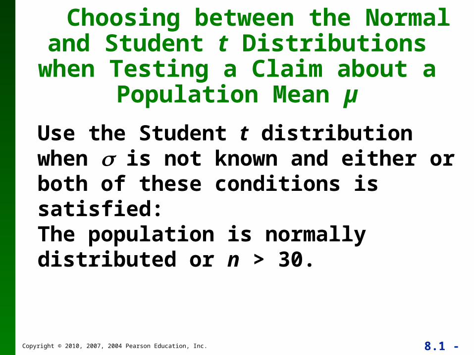
Choosing between the Normal and Student t Distributions when Testing a
Claim about a Population Mean µ
Use the Student t distribution when is not known and either or both of these conditions is satisfied:The population is normally distributed or n > 30.
Copyright © 2010, 2007, 2004 Pearson Education, Inc. 8.1 - 110
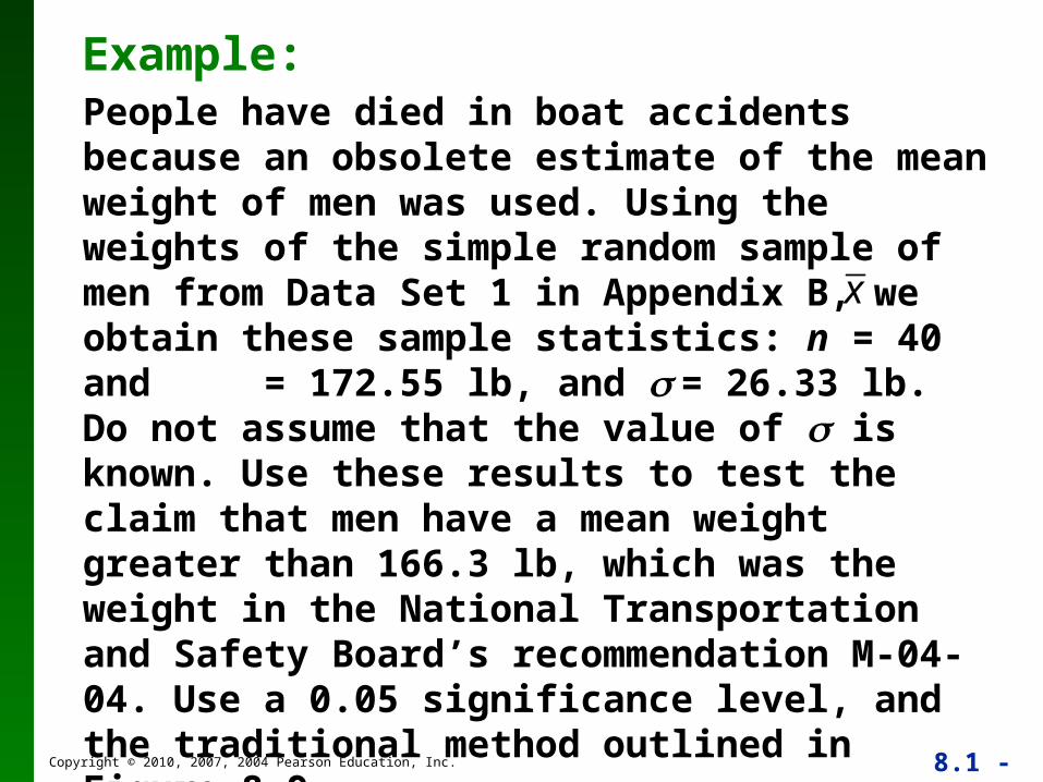
Example:People have died in boat accidents because an obsolete estimate of the mean weight of men was used. Using the weights of the simple random sample of men from Data Set 1 in Appendix B, we obtain these sample statistics: n = 40 and = 172.55 lb, and = 26.33 lb. Do not assume that the value of is known. Use these results to test the claim that men have a mean weight greater than 166.3 lb, which was the weight in the National Transportation and Safety Board’s recommendation M-04-04. Use a 0.05 significance level, and the traditional method outlined in Figure 8-9.
x
Copyright © 2010, 2007, 2004 Pearson Education, Inc. 8.1 - 111
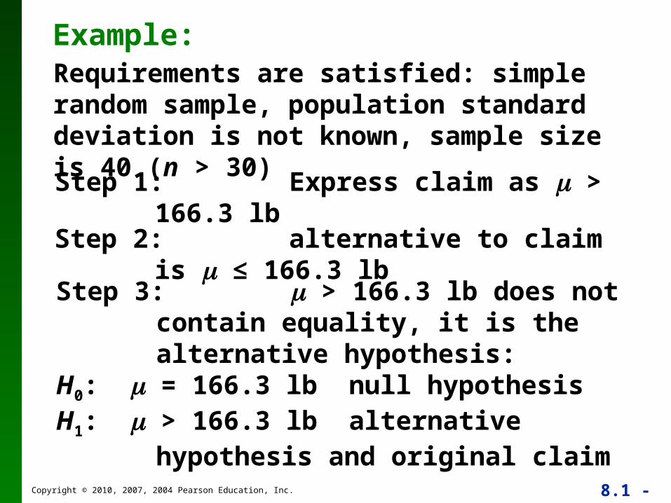
Example:Requirements are satisfied: simple random sample, population standard deviation is not known, sample size is 40 (n > 30)
Step 1: Express claim as > 166.3 lb
Step 2: alternative to claim is ≤ 166.3 lb
Step 3: > 166.3 lb does not contain equality, it is the alternative hypothesis:
H0: = 166.3 lb null hypothesisH1: > 166.3 lb alternative hypothesis and
original claim
Copyright © 2010, 2007, 2004 Pearson Education, Inc. 8.1 - 112
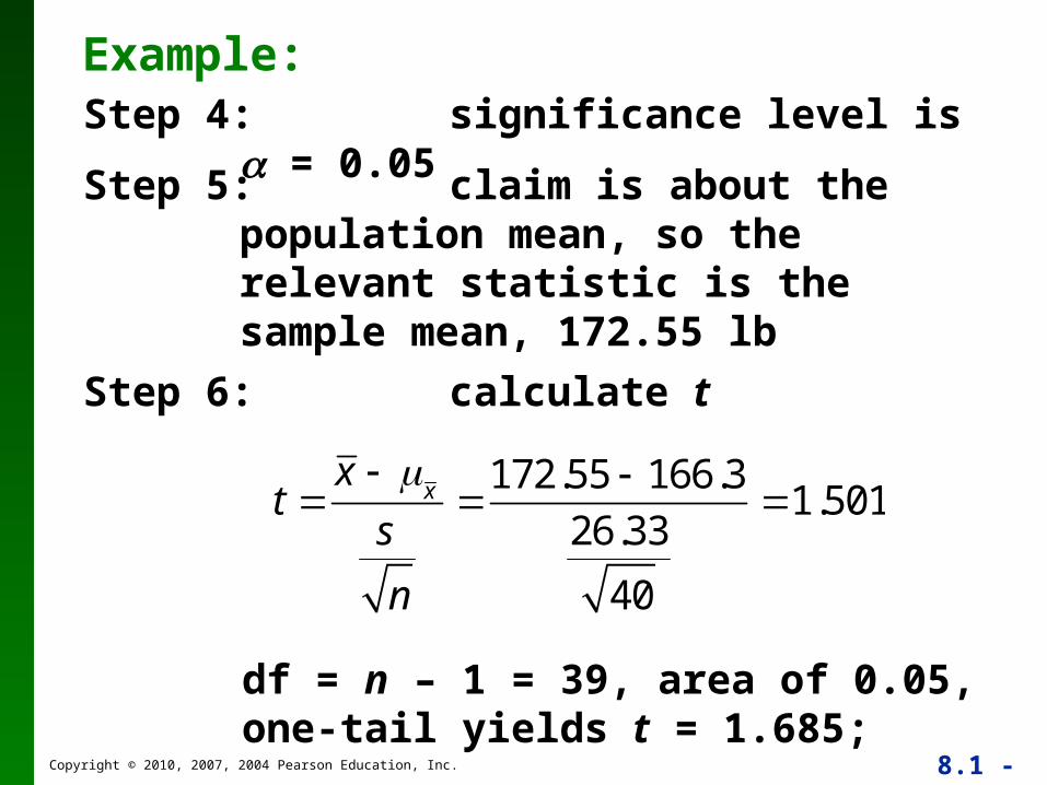
Example:Step 4: significance level is = 0.05
Step 5: claim is about the population mean, so the relevant statistic is the sample mean, 172.55 lb
Step 6: calculate t
t x
x
s
n
172.55 166.3
26.33
40
1.501
df = n – 1 = 39, area of 0.05, one-tail yields t = 1.685;

Copyright © 2010, 2007, 2004 Pearson Education, Inc. 8.1 - 113
Example:
Step 7: t = 1.501 does not fall in the critical region bounded by t = 1.685, we fail to reject the null hypothesis.
= 166.3or
z = 0 x 172.55
ort = 1.52
Critical value t = 1.685
Copyright © 2010, 2007, 2004 Pearson Education, Inc. 8.1 - 114
Example:
Because we fail to reject the null hypothesis, we conclude that there is not sufficient evidence to support a conclusion that the population mean is greater than 166.3 lb, as in the National Transportation and Safety Board’s recommendation.

Copyright © 2010, 2007, 2004 Pearson Education, Inc. 8.1 - 115
The critical value in the preceding example was t = 1.782, but if the normal distribution were being used, the critical value would have been z = 1.645.
The Student t critical value is larger (farther to the right), showing that with the Student t distribution, the sample evidence must be more extreme before we can consider it to be significant.
Normal Distribution Versus Student t Distribution
Copyright © 2010, 2007, 2004 Pearson Education, Inc. 8.1 - 116
P-Value Method
Use software or a TI-83/84 Plus calculator.
If technology is not available, use Table A-3 to identify a range of P-values.
Copyright © 2010, 2007, 2004 Pearson Education, Inc. 8.1 - 117
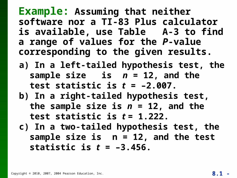
a) In a left-tailed hypothesis test, the sample size is n = 12, and the test statistic is t = –2.007.
b) In a right-tailed hypothesis test, the sample size is n = 12, and the test statistic is t = 1.222.
c) In a two-tailed hypothesis test, the sample size is n = 12, and the test statistic is t = –3.456.
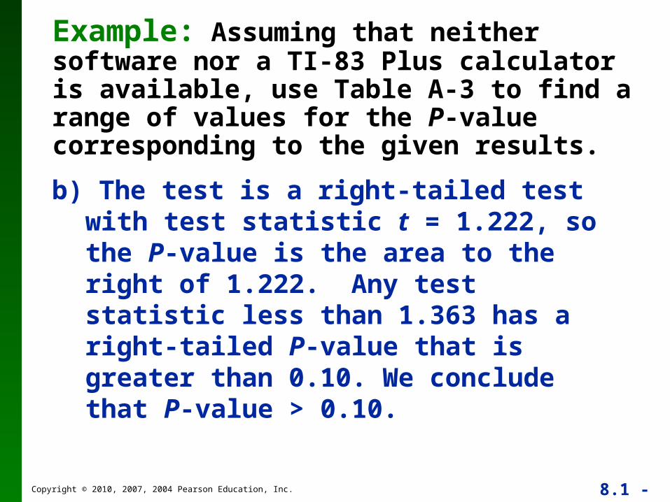
Example: Assuming that neither software nor a TI-83 Plus calculator is available, use Table A-3 to find a range of values for the P-value corresponding to the given results.
Copyright © 2010, 2007, 2004 Pearson Education, Inc. 8.1 - 118
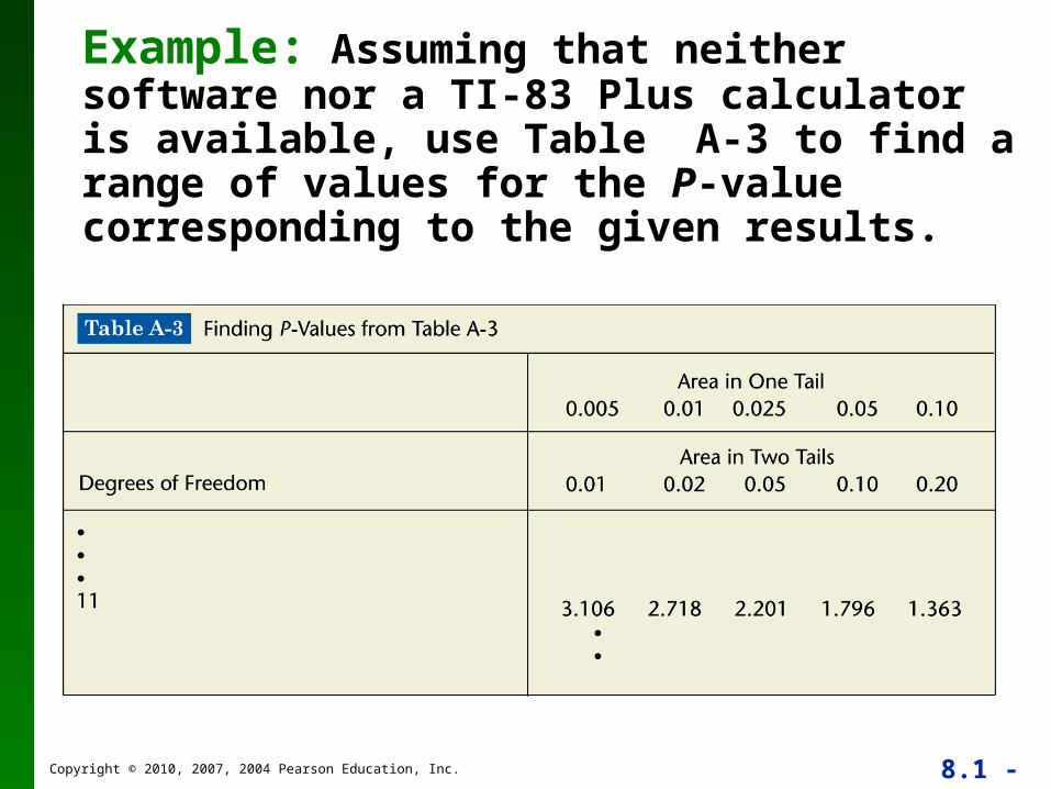
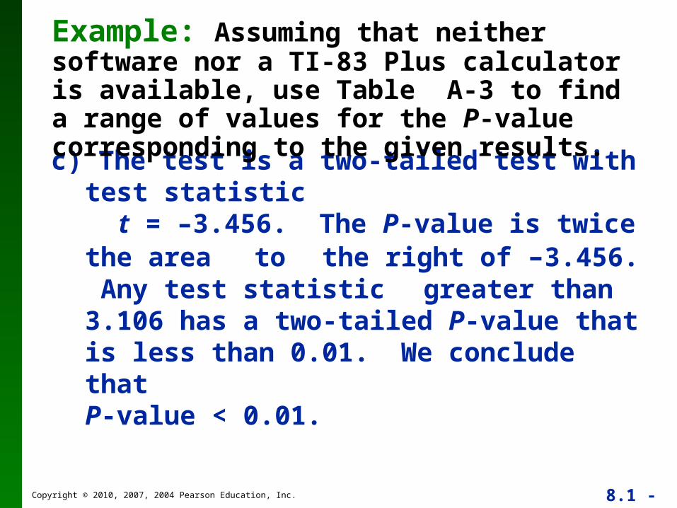
Example: Assuming that neither software nor a TI-83 Plus calculator is available, use Table A-3 to find a range of values for the P-value corresponding to the given results.
Copyright © 2010, 2007, 2004 Pearson Education, Inc. 8.1 - 119
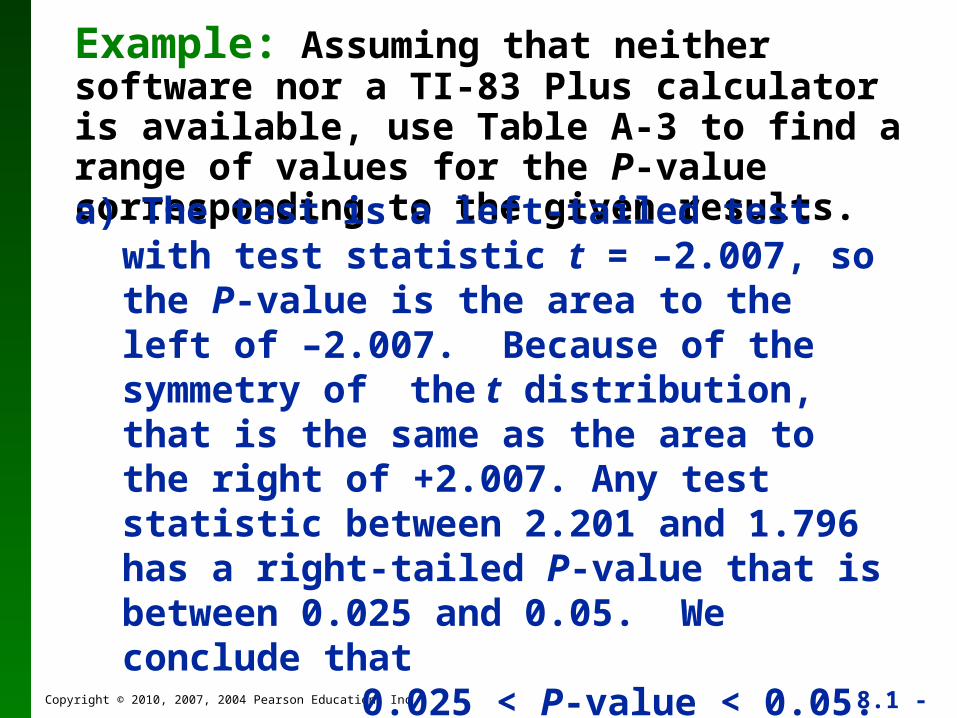
Example: Assuming that neither software nor a TI-83 Plus calculator is available, use Table A-3 to find a range of values for the P-value corresponding to the given results.
a) The test is a left-tailed test with test statistic t = –2.007, so the P-value is the area to the left of –2.007. Because of the symmetry of the t distribution, that is the same as the area to the right of +2.007. Any test statistic between 2.201 and 1.796 has a right-tailed P-value that is between 0.025 and 0.05. We conclude that
0.025 < P-value < 0.05.
Copyright © 2010, 2007, 2004 Pearson Education, Inc. 8.1 - 120
Example: Assuming that neither software nor a TI-83 Plus calculator is available, use Table A-3 to find a range of values for the P-value corresponding to the given results.
b) The test is a right-tailed test with test statistic t = 1.222, so the P-value is the area to the right of 1.222. Any test statistic less than 1.363 has a right-tailed P-value that is greater than 0.10. We conclude that P-value > 0.10.
Copyright © 2010, 2007, 2004 Pearson Education, Inc. 8.1 - 121
c) The test is a two-tailed test with test statistic
t = –3.456. The P-value is twice the area to the right of –3.456. Any test statistic greater than 3.106 has a two-tailed P-value that is less than 0.01. We conclude thatP-value < 0.01.
Example: Assuming that neither software nor a TI-83 Plus calculator is available, use Table A-3 to find a range of values for the P-value corresponding to the given results.
Copyright © 2010, 2007, 2004 Pearson Education, Inc. 8.1 - 122
Recap
In this section we have discussed:
Assumptions for testing claims about population means, σ unknown.
Student t distribution.
P-value method.
Copyright © 2010, 2007, 2004 Pearson Education, Inc. 8.1 - 123
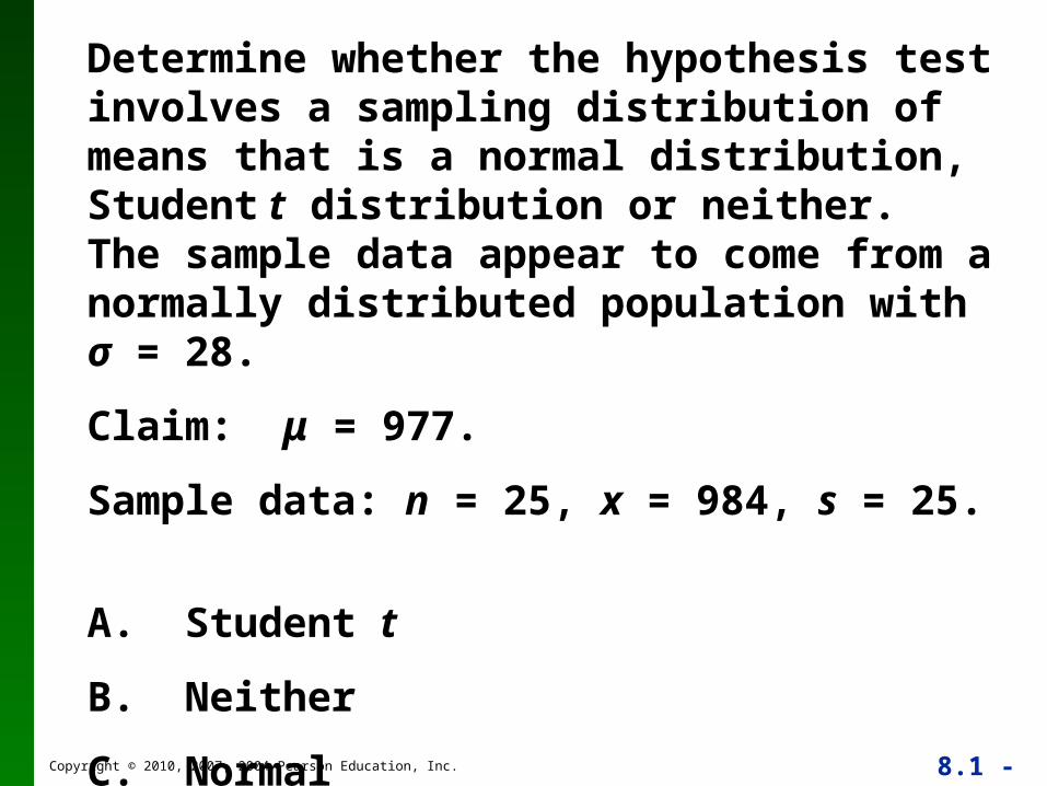
Determine whether the hypothesis test involves a sampling distribution of means that is a normal distribution, Student t distribution or neither. The sample data appear to come from a normally distributed population with σ = 28.
Claim: μ = 977.
Sample data: n = 25, x = 984, s = 25.
A. Student t
B. Neither
C. Normal

Copyright © 2010, 2007, 2004 Pearson Education, Inc. 8.1 - 124
Section 8-6 Testing a Claim About a Standard Deviation or
Variance
Copyright © 2010, 2007, 2004 Pearson Education, Inc. 8.1 - 125
Key Concept
This section introduces methods for testing a claim made about a population standard deviation σ or population variance σ
2. The methods of this section use the chi-square distribution that was first introduced in Section 7-5.
Copyright © 2010, 2007, 2004 Pearson Education, Inc. 8.1 - 126
Requirements for Testing Claims About or 2
n = sample size
s = sample standard deviation
s2 = sample variance
= claimed value of the population standard
deviation
2 = claimed value of the population variance
Copyright © 2010, 2007, 2004 Pearson Education, Inc. 8.1 - 127
Requirements for Testing Claims About or 2
1. The sample is a simple random sample.
2. The population has a normal distribution. (This is a much stricter requirement than the requirement of a normal distribution when testing claims about means.)
Copyright © 2010, 2007, 2004 Pearson Education, Inc. 8.1 - 128
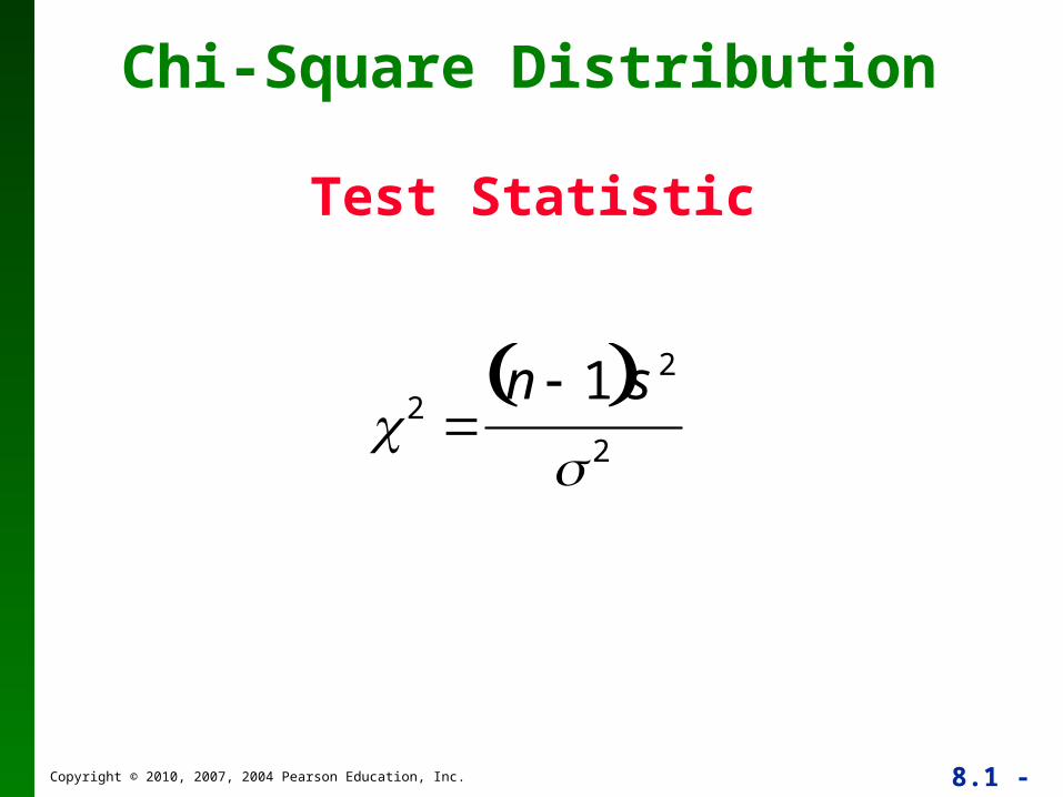
Chi-Square Distribution
Test Statistic
2
n 1 s2
2

Copyright © 2010, 2007, 2004 Pearson Education, Inc. 8.1 - 129
P-Values and Critical Values for
Chi-Square Distribution
• Use Table A-4.
• The degrees of freedom = n –1.
Copyright © 2010, 2007, 2004 Pearson Education, Inc. 8.1 - 130
Caution
The 2 test of this section is not robust against a departure from normality, meaning that the test does not work well if the population has a distribution that is far from normal. The condition of a normally distributed population is therefore a much stricter requirement in this section than it was in Sections 8-4 and 8-5.
Copyright © 2010, 2007, 2004 Pearson Education, Inc. 8.1 - 131
Properties of Chi-Square Distribution
• All values of 2 are nonnegative, and the
distribution is not symmetric (see Figure 8-13, following).
• There is a different distribution for each number of degrees of freedom (see Figure 8-14, following).
• The critical values are found in Table A-4 using n – 1 degrees of freedom.
Copyright © 2010, 2007, 2004 Pearson Education, Inc. 8.1 - 132
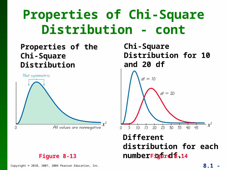
Properties of Chi-Square Distribution - cont
Figure 8-13
Properties of the Chi-Square Distribution
Different distribution for each number of df.
Chi-Square Distribution for 10 and 20 df
Figure 8-14
Copyright © 2010, 2007, 2004 Pearson Education, Inc. 8.1 - 133
Table A-4Table A-4 is based on cumulative areas from the right (unlike the entries in Table A-2, which are cumulative areas from the left). Critical values are found in Table A-4 by first locating the row corresponding to the appropriate number of degrees of freedom (where df = n –1). Next, the significance level is used to determine the correct column. The following examples are based on a significance level of = 0.05, but any other significance level can be used in a similar manner.
Copyright © 2010, 2007, 2004 Pearson Education, Inc. 8.1 - 134
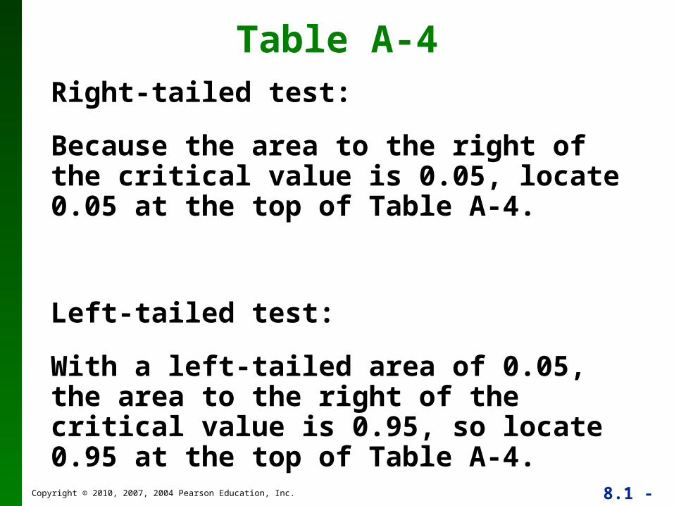
Table A-4Right-tailed test:
Because the area to the right of the critical value is 0.05, locate 0.05 at the top of Table A-4.
Left-tailed test:
With a left-tailed area of 0.05, the area to the right of the critical value is 0.95, so locate 0.95 at the top of Table A-4.

Copyright © 2010, 2007, 2004 Pearson Education, Inc. 8.1 - 135
Table A-4Two-tailed test:
Unlike the normal and Student t distributions, the critical values in this 2
test will be two different positive values (instead of something like ±1.96 ). Divide a significance level of 0.05 between the left and right tails, so the areas to the right of the two critical values are 0.975 and 0.025, respectively. Locate 0.975 and 0.025 at the top of Table A-4

Copyright © 2010, 2007, 2004 Pearson Education, Inc. 8.1 - 136
Example:
A common goal in business and industry is to improve the quality of goods or services by reducing variation. Quality control engineers want to ensure that a product has an acceptable mean, but they also want to produce items of consistent quality so that there will be few defects. If weights of coins have a specified mean but too much variation, some will have weights that are too low or too high, so that vending machines will not work correctly (unlike the stellar performance that they now provide).
Copyright © 2010, 2007, 2004 Pearson Education, Inc. 8.1 - 137
Example:
Consider the simple random sample of the 37 weights of post-1983 pennies listed in Data Set 20 in Appendix B. Those 37 weights have a mean of 2.49910 g and a standard deviation of 0.01648 g. U.S. Mint specifications require that pennies be manufactured so that the mean weight is 2.500 g. A hypothesis test will verify that the sample appears to come from a population with a mean of 2.500 g as required, but use a 0.05 significance level to test the claim that the population of weights has a standard deviation less than the specification of 0.0230 g.
Copyright © 2010, 2007, 2004 Pearson Education, Inc. 8.1 - 138
Example:
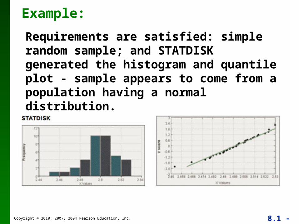
Requirements are satisfied: simple random sample; and STATDISK generated the histogram and quantile plot - sample appears to come from a population having a normal distribution.
Copyright © 2010, 2007, 2004 Pearson Education, Inc. 8.1 - 139
Example:
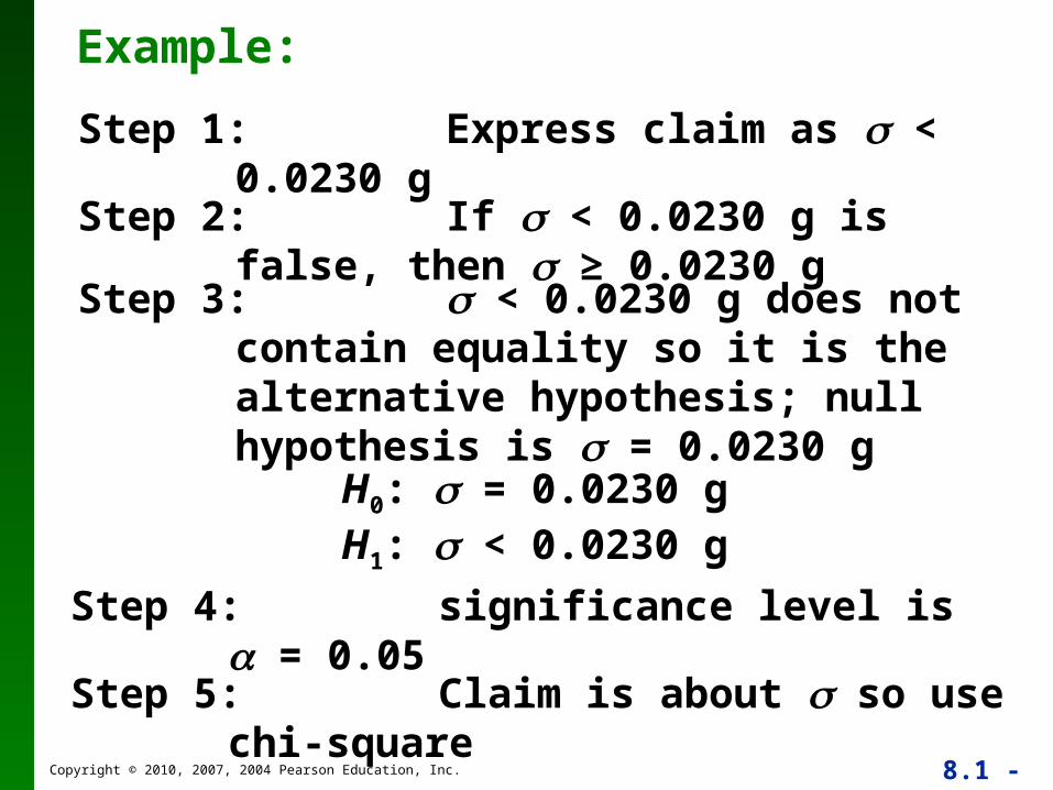
Step 1: Express claim as < 0.0230 g
Step 2: If < 0.0230 g is false, then ≥ 0.0230 g
Step 3: < 0.0230 g does not contain equality so it is the alternative hypothesis; null hypothesis is = 0.0230 g
H0: = 0.0230 gH1: < 0.0230 g
Step 4: significance level is = 0.05
Step 5: Claim is about so use chi-square
Copyright © 2010, 2007, 2004 Pearson Education, Inc. 8.1 - 140
Example:
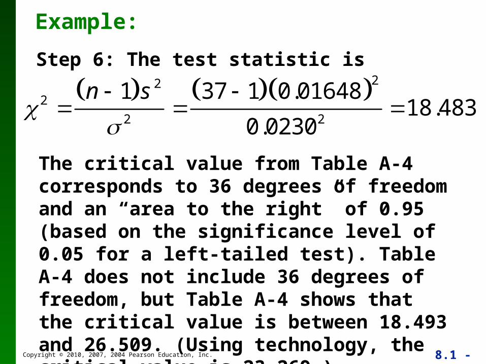
Step 6: The test statistic is
The critical value from Table A-4 corresponds to 36 degrees of freedom and an “area to the right” of 0.95 (based on the significance level of 0.05 for a left-tailed test). Table A-4 does not include 36 degrees of freedom, but Table A-4 shows that the critical value is between 18.493 and 26.509. (Using technology, the critical value is 23.269.)
22
2
2 2
1 37 1 0.0164818.483
0.0230
n s
Copyright © 2010, 2007, 2004 Pearson Education, Inc. 8.1 - 141
Example:
Copyright © 2010, 2007, 2004 Pearson Education, Inc. 8.1 - 142
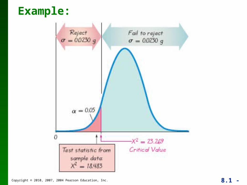
Example:
Step 7: Because the test statistic is in the critical region, reject the null hypothesis.
There is sufficient evidence to support the claim that the standard deviation of weights is less than 0.0230 g. It appears that the variation is less than 0.0230 g as specified, so the manufacturing process is acceptable.
Copyright © 2010, 2007, 2004 Pearson Education, Inc. 8.1 - 143
Recap
In this section we have discussed:
Tests for claims about standard deviation and variance.
Test statistic.
Chi-square distribution.
Critical values.
Copyright © 2010, 2007, 2004 Pearson Education, Inc. 8.1 - 144
Find the critical value or values of χ2 based on the given information. H1: σ > 26.1, n = 9, α = 0.01
A. 20.090
B. 21.666
C. 1.646
D. 2.088