Convergence in DistributionCentral Limit Theorem

Statistics 110

Summer 2006

Copyright c©2006 by Mark E. Irwin

Convergence in Distribution

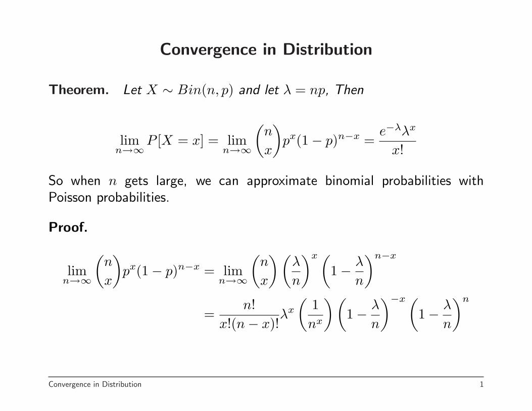
Theorem. Let X ∼ Bin(n, p) and let λ = np, Then

limn→∞

P [X = x] = limn→∞

(n

x

)px(1− p)n−x =

e−λλx

x!

So when n gets large, we can approximate binomial probabilities withPoisson probabilities.

Proof.

limn→∞

(n

x

)px(1− p)n−x = lim

n→∞

(n

x

)(λ

n

)x (1− λ

n

)n−x

=n!

x!(n− x)!λx

(1nx

)(1− λ

n

)−x (1− λ

n

)n

Convergence in Distribution 1

=n!

x!(n− x)!λx

(1nx

)(1− λ

n

)−x (1− λ

n

)n

=λx

x!lim

n→∞n!

(n− x)!1

(n− λ)x︸ ︷︷ ︸→1

(1− λ

n

)n

︸ ︷︷ ︸→e−λ

=e−λλx

x!

2

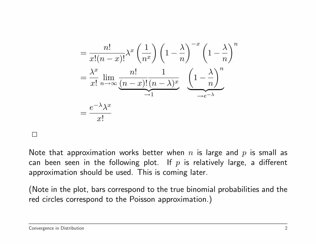
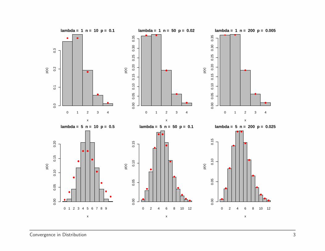
Note that approximation works better when n is large and p is small ascan been seen in the following plot. If p is relatively large, a differentapproximation should be used. This is coming later.

(Note in the plot, bars correspond to the true binomial probabilities and thered circles correspond to the Poisson approximation.)

Convergence in Distribution 2

0 1 2 3 4

lambda = 1 n = 10 p = 0.1

x

p(x)

0.0

0.1

0.2

0.3

0 1 2 3 4

lambda = 1 n = 50 p = 0.02

x

p(x)

0.00

0.05

0.10

0.15

0.20

0.25

0.30

0.35

0 1 2 3 4

lambda = 1 n = 200 p = 0.005

x

p(x)

0.00

0.05

0.10

0.15

0.20

0.25

0.30

0.35

0 1 2 3 4 5 6 7 8 9

lambda = 5 n = 10 p = 0.5

x

p(x)

0.00

0.05

0.10

0.15

0.20

0 2 4 6 8 10 12

lambda = 5 n = 50 p = 0.1

x

p(x)

0.00

0.05

0.10

0.15

0 2 4 6 8 10 12

lambda = 5 n = 200 p = 0.025

x

p(x)

0.00

0.05

0.10

0.15

Convergence in Distribution 3

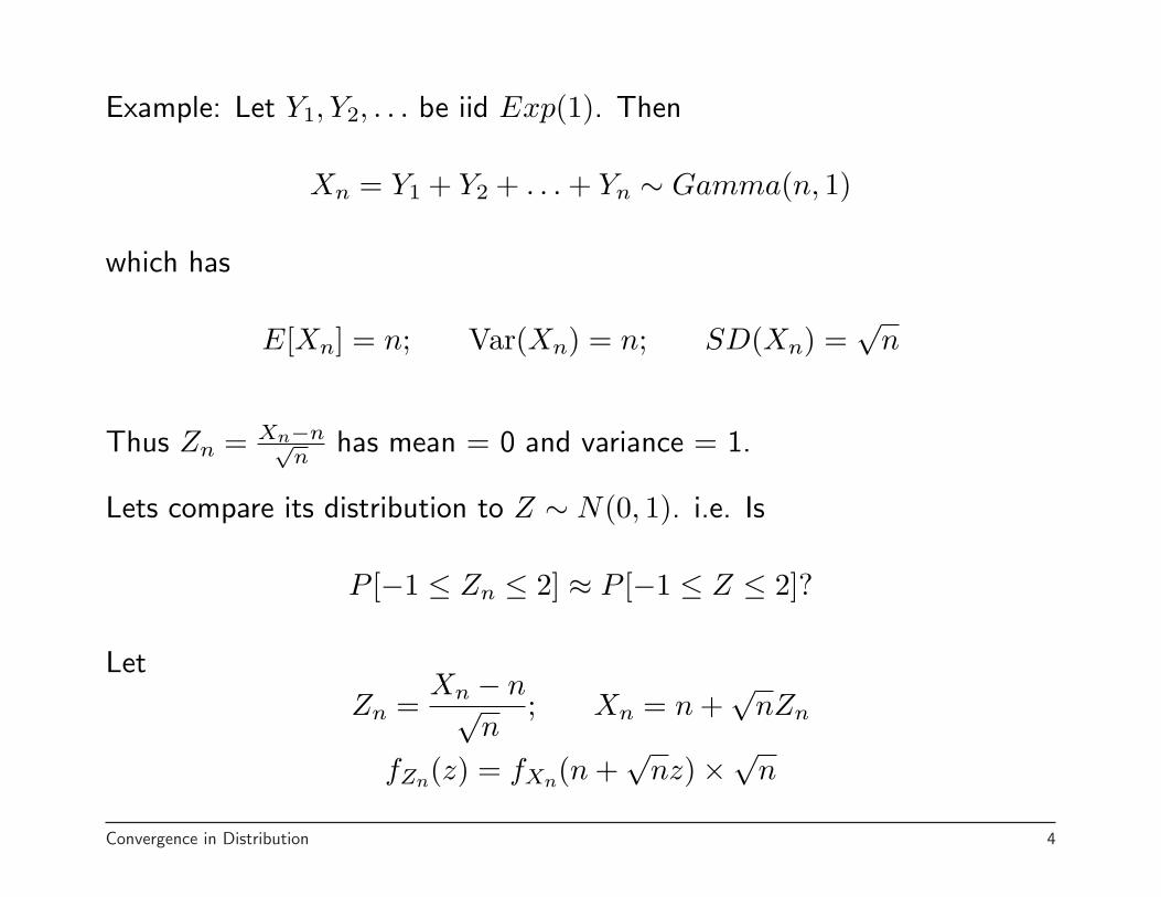
Example: Let Y1, Y2, . . . be iid Exp(1). Then

Xn = Y1 + Y2 + . . . + Yn ∼ Gamma(n, 1)

which has

E[Xn] = n; Var(Xn) = n; SD(Xn) =√

n

Thus Zn = Xn−n√n

has mean = 0 and variance = 1.

Lets compare its distribution to Z ∼ N(0, 1). i.e. Is

P [−1 ≤ Zn ≤ 2] ≈ P [−1 ≤ Z ≤ 2]?

Let

Zn =Xn − n√

n; Xn = n +

√nZn

fZn(z) = fXn(n +√

nz)×√n

Convergence in Distribution 4

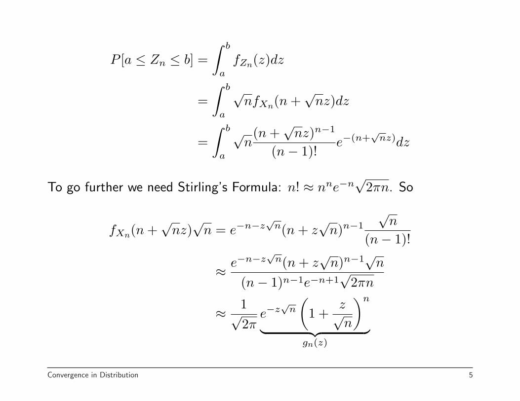
P [a ≤ Zn ≤ b] =∫ b

a

fZn(z)dz

=∫ b

a

√nfXn(n +

√nz)dz

=∫ b

a

√n(n +

√nz)n−1

(n− 1)!e−(n+

√nz)dz

To go further we need Stirling’s Formula: n! ≈ nne−n√

2πn. So

fXn(n +√

nz)√

n = e−n−z√

n(n + z√

n)n−1

√n

(n− 1)!

≈ e−n−z√

n(n + z√

n)n−1√

n

(n− 1)n−1e−n+1√

2πn

≈ 1√2π

e−z√

n

(1 +

z√n

)n

︸ ︷︷ ︸gn(z)

Convergence in Distribution 5

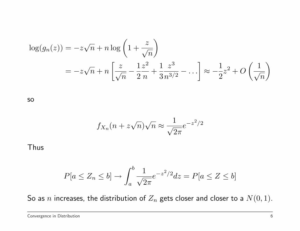
log(gn(z)) = −z√

n + n log(

1 +z√n

)

= −z√

n + n

[z√n− 1

2z2

n+

13

z3

n3/2− . . .

]≈ −1

2z2 + O

(1√n

)

so

fXn(n + z√

n)√

n ≈ 1√2π

e−z2/2

Thus

P [a ≤ Zn ≤ b] →∫ b

a

1√2π

e−z2/2dz = P [a ≤ Z ≤ b]

So as n increases, the distribution of Zn gets closer and closer to a N(0, 1).

Convergence in Distribution 6

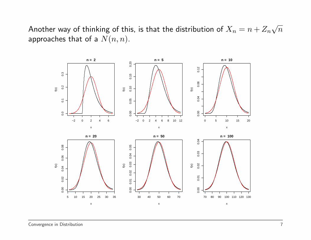
Another way of thinking of this, is that the distribution of Xn = n + Zn√

napproaches that of a N(n, n).

−2 0 2 4 6

0.0

0.1

0.2

0.3

n = 2

x

f(x)

−2 0 2 4 6 8 10 12

0.00

0.05

0.10

0.15

0.20

n = 5

xf(

x)0 5 10 15 20

0.00

0.04

0.08

0.12

n = 10

x

f(x)

5 10 15 20 25 30 35

0.00

0.02

0.04

0.06

0.08

n = 20

x

f(x)

30 40 50 60 70

0.00

0.01

0.02

0.03

0.04

0.05

n = 50

x

f(x)

70 80 90 100 110 120 1300.

000.

010.

020.

030.

04

n = 100

x

f(x)

Convergence in Distribution 7

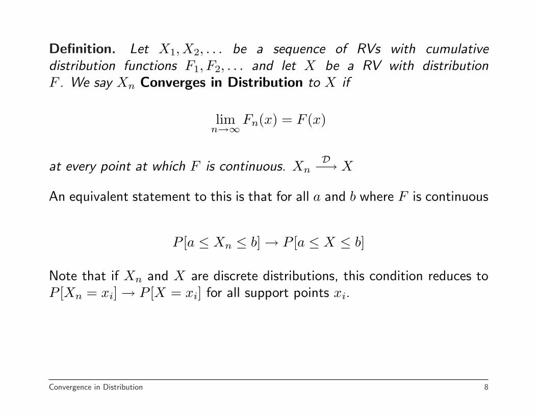
Definition. Let X1, X2, . . . be a sequence of RVs with cumulativedistribution functions F1, F2, . . . and let X be a RV with distributionF . We say Xn Converges in Distribution to X if

limn→∞

Fn(x) = F (x)

at every point at which F is continuous. XnD−→ X

An equivalent statement to this is that for all a and b where F is continuous

P [a ≤ Xn ≤ b] → P [a ≤ X ≤ b]

Note that if Xn and X are discrete distributions, this condition reduces toP [Xn = xi] → P [X = xi] for all support points xi.

Convergence in Distribution 8

Note that an equivalent definition of convergence in distribution is that

XnD−→ X if E[g(Xn)] → E[g(X)] for all bounded, continuous functions

g(·).This statement of convergence in distribution is needed to help prove thefollowing theorem

Theorem. [Continuity Theorem] Let Xn be a sequence of randomvariables with cumulative distribution functions Fn(x) and correspondingmoment generating functions Mn(t). Let X be a random variable withcumulative distribution function F (x) and moment generating functionM(t). If Mn(t) → M(t) for all t in an open interval containing zero, then

Fn(x) → F (x) at all continuity points of F . That is XnD−→ X.

Thus the previous two examples (Binomial/Poisson and Gamma/Normal)could be proved this way.

Convergence in Distribution 9

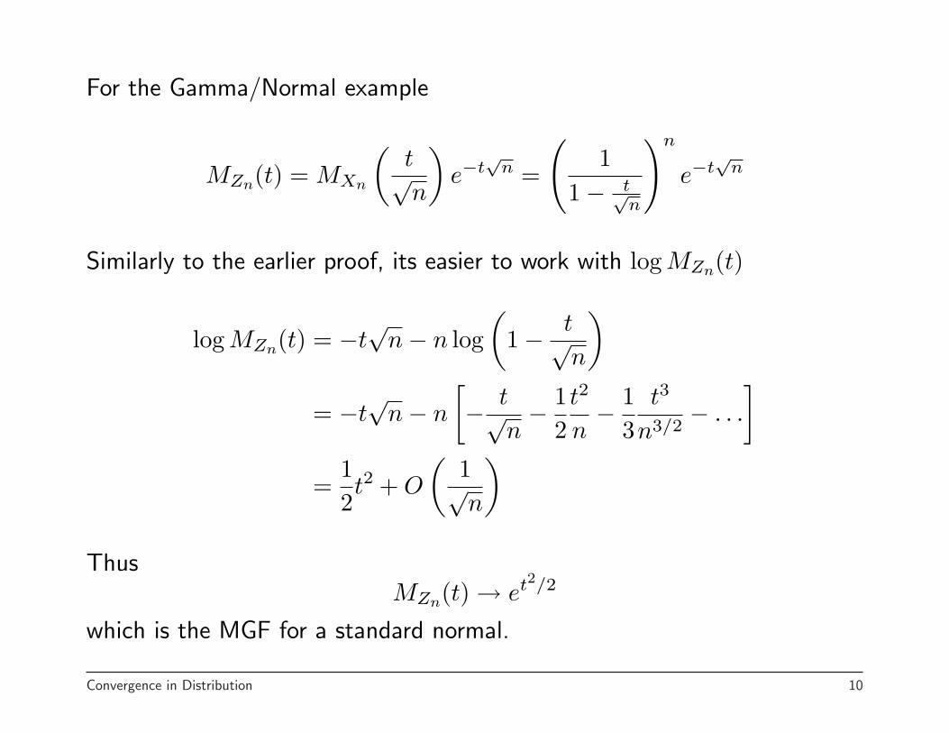
For the Gamma/Normal example

MZn(t) = MXn

(t√n

)e−t

√n =

(1

1− t√n

)n

e−t√

n

Similarly to the earlier proof, its easier to work with log MZn(t)

log MZn(t) = −t√

n− n log(

1− t√n

)

= −t√

n− n

[− t√

n− 1

2t2

n− 1

3t3

n3/2− . . .

]

=12t2 + O

(1√n

)

ThusMZn(t) → et2/2

which is the MGF for a standard normal.

Convergence in Distribution 10

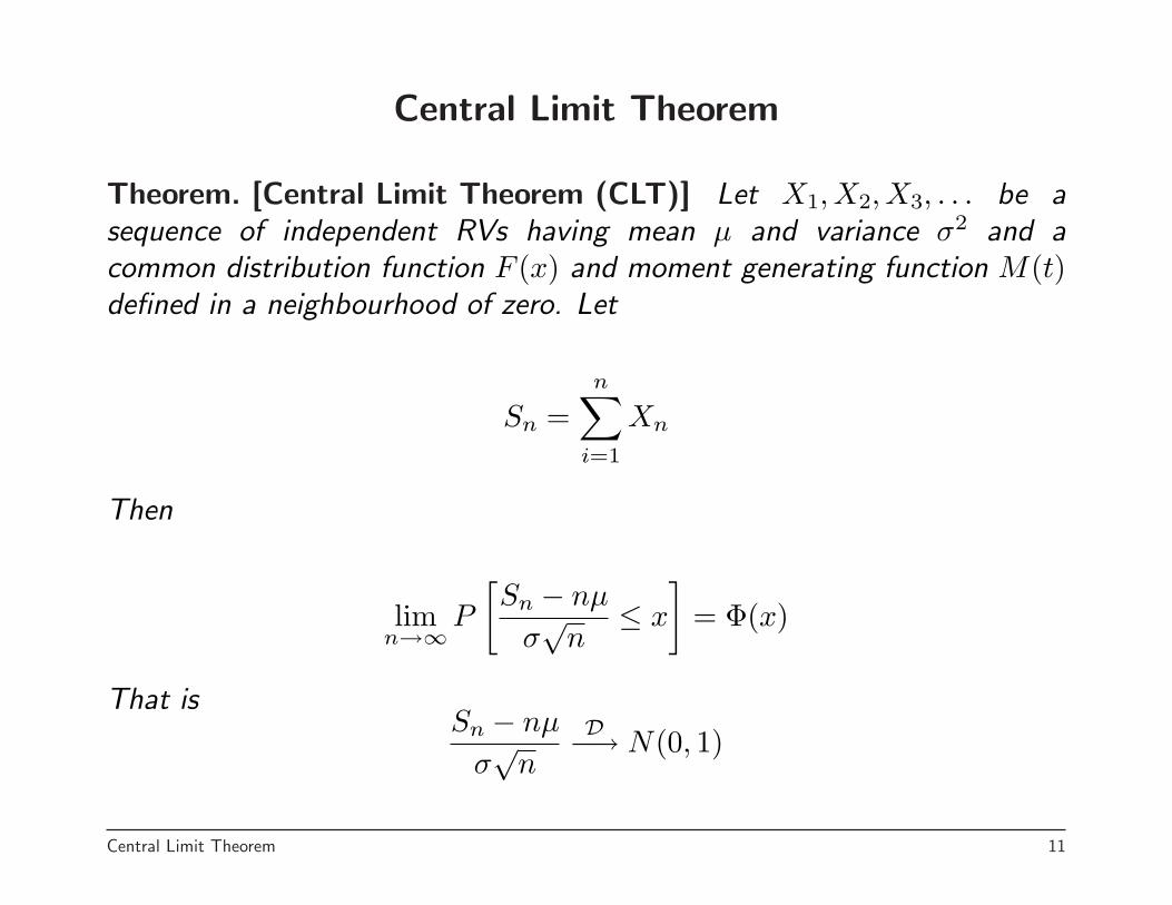
Central Limit Theorem

Theorem. [Central Limit Theorem (CLT)] Let X1, X2, X3, . . . be asequence of independent RVs having mean µ and variance σ2 and acommon distribution function F (x) and moment generating function M(t)defined in a neighbourhood of zero. Let

Sn =n∑

i=1

Xn

Then

limn→∞

P

[Sn − nµ

σ√

n≤ x

]= Φ(x)

That isSn − nµ

σ√

n

D−→ N(0, 1)

Central Limit Theorem 11

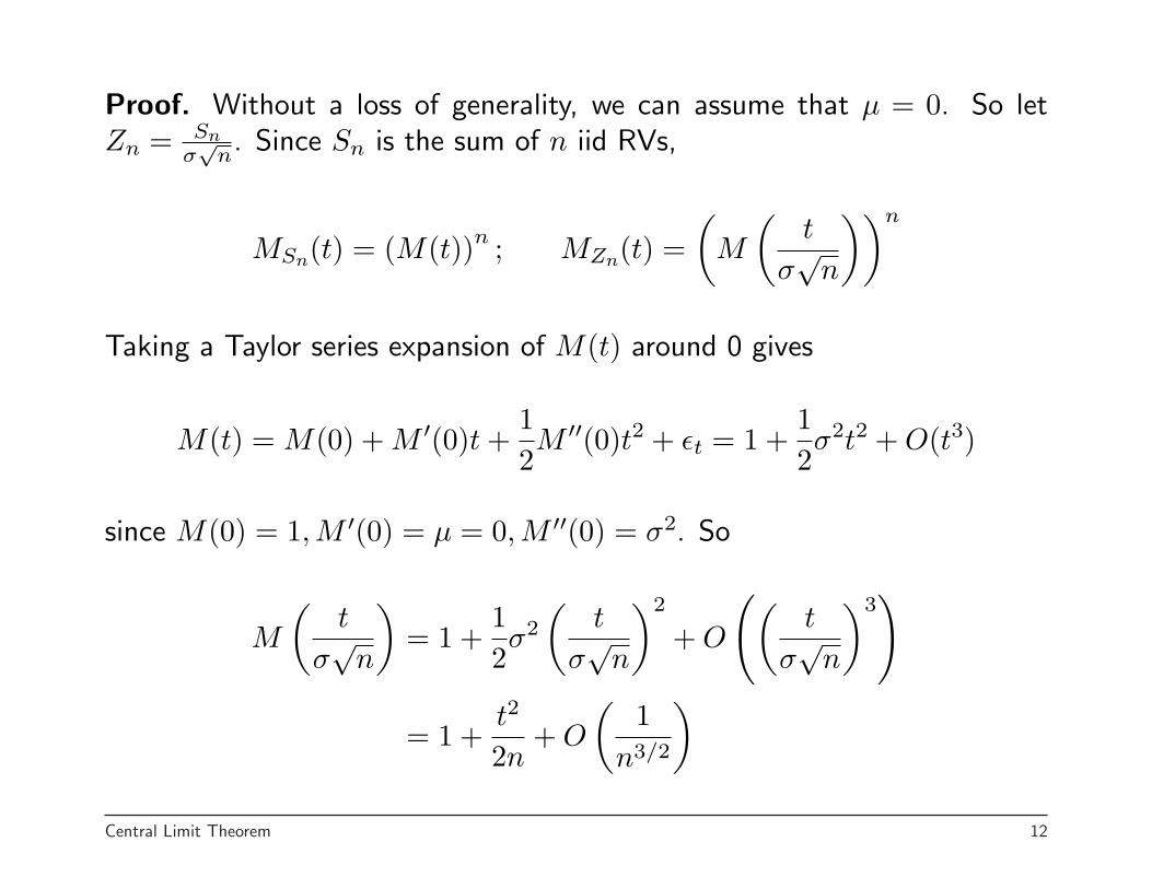
Proof. Without a loss of generality, we can assume that µ = 0. So letZn = Sn

σ√

n. Since Sn is the sum of n iid RVs,

MSn(t) = (M(t))n ; MZn(t) =(

M

(t

σ√

n

))n

Taking a Taylor series expansion of M(t) around 0 gives

M(t) = M(0) + M ′(0)t +12M ′′(0)t2 + εt = 1 +

12σ2t2 + O(t3)

since M(0) = 1,M ′(0) = µ = 0,M ′′(0) = σ2. So

M

(t

σ√

n

)= 1 +

12σ2

(t

σ√

n

)2

+ O

((t

σ√

n

)3)

= 1 +t2

2n+ O

(1

n3/2

)

Central Limit Theorem 12

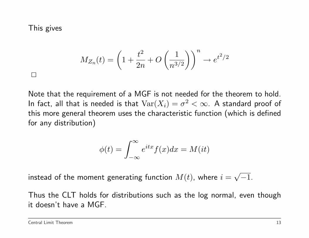
This gives

MZn(t) =(

1 +t2

2n+ O

(1

n3/2

))n

→ et2/2

2

Note that the requirement of a MGF is not needed for the theorem to hold.In fact, all that is needed is that Var(Xi) = σ2 < ∞. A standard proof ofthis more general theorem uses the characteristic function (which is definedfor any distribution)

φ(t) =∫ ∞

−∞eitxf(x)dx = M(it)

instead of the moment generating function M(t), where i =√−1.

Thus the CLT holds for distributions such as the log normal, even thoughit doesn’t have a MGF.

Central Limit Theorem 13

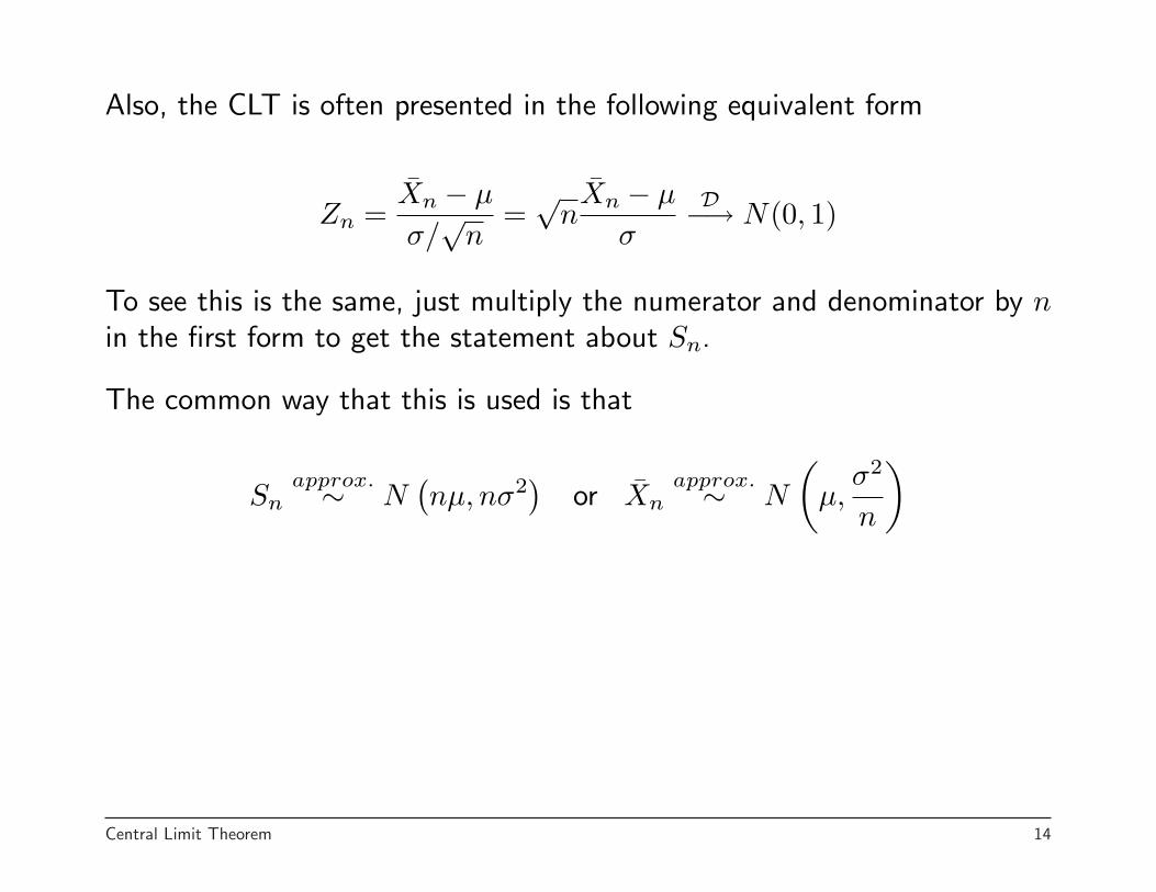
Also, the CLT is often presented in the following equivalent form

Zn =X̄n − µ

σ/√

n=√

nX̄n − µ

σ

D−→ N(0, 1)

To see this is the same, just multiply the numerator and denominator by nin the first form to get the statement about Sn.

The common way that this is used is that

Snapprox.∼ N

(nµ, nσ2

)or X̄n

approx.∼ N

(µ,

σ2

n

)

Central Limit Theorem 14

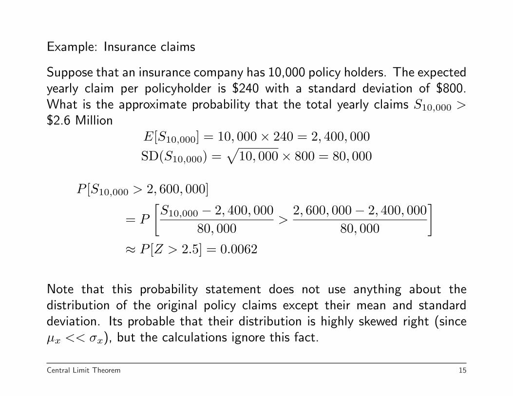
Example: Insurance claims

Suppose that an insurance company has 10,000 policy holders. The expectedyearly claim per policyholder is $240 with a standard deviation of $800.What is the approximate probability that the total yearly claims S10,000 >$2.6 Million

E[S10,000] = 10, 000× 240 = 2, 400, 000SD(S10,000) =

√10, 000× 800 = 80, 000

P [S10,000 > 2, 600, 000]

= P

[S10,000 − 2, 400, 000

80, 000>

2, 600, 000− 2, 400, 00080, 000

]

≈ P [Z > 2.5] = 0.0062

Note that this probability statement does not use anything about thedistribution of the original policy claims except their mean and standarddeviation. Its probable that their distribution is highly skewed right (sinceµx << σx), but the calculations ignore this fact.

Central Limit Theorem 15

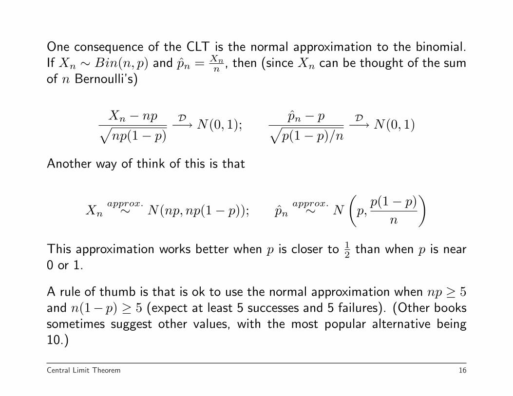
One consequence of the CLT is the normal approximation to the binomial.If Xn ∼ Bin(n, p) and p̂n = Xn

n , then (since Xn can be thought of the sumof n Bernoulli’s)

Xn − np√np(1− p)

D−→ N(0, 1);p̂n − p√

p(1− p)/n

D−→ N(0, 1)

Another way of think of this is that

Xnapprox.∼ N(np, np(1− p)); p̂n

approx.∼ N

(p,

p(1− p)n

)

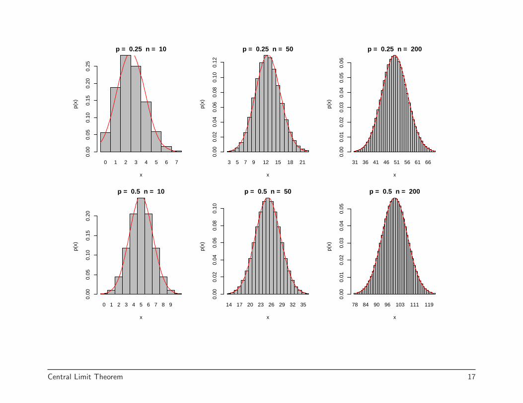
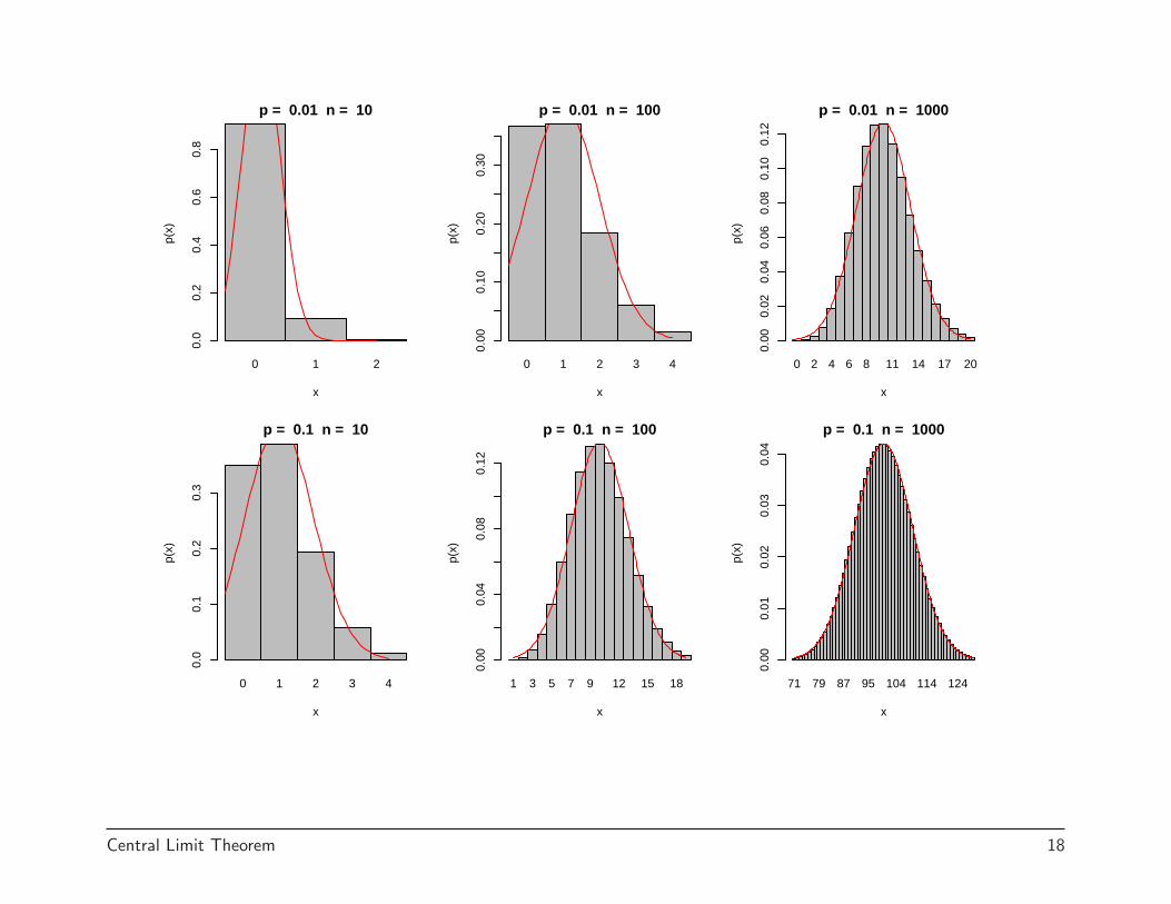
This approximation works better when p is closer to 12 than when p is near

0 or 1.

A rule of thumb is that is ok to use the normal approximation when np ≥ 5and n(1− p) ≥ 5 (expect at least 5 successes and 5 failures). (Other bookssometimes suggest other values, with the most popular alternative being10.)

Central Limit Theorem 16

0 1 2 3 4 5 6 7

p = 0.25 n = 10

x

p(x)

0.00

0.05

0.10

0.15

0.20

0.25

3 5 7 9 12 15 18 21

p = 0.25 n = 50

x

p(x)

0.00

0.02

0.04

0.06

0.08

0.10

0.12

31 36 41 46 51 56 61 66

p = 0.25 n = 200

x

p(x)

0.00

0.01

0.02

0.03

0.04

0.05

0.06

0 1 2 3 4 5 6 7 8 9

p = 0.5 n = 10

x

p(x)

0.00

0.05

0.10

0.15

0.20

14 17 20 23 26 29 32 35

p = 0.5 n = 50

x

p(x)

0.00

0.02

0.04

0.06

0.08

0.10

78 84 90 96 103 111 119

p = 0.5 n = 200

x

p(x)

0.00

0.01

0.02

0.03

0.04

0.05

Central Limit Theorem 17

0 1 2

p = 0.01 n = 10

x

p(x)

0.0

0.2

0.4

0.6

0.8

0 1 2 3 4

p = 0.01 n = 100

x

p(x)

0.00

0.10

0.20

0.30

0 2 4 6 8 11 14 17 20

p = 0.01 n = 1000

x

p(x)

0.00

0.02

0.04

0.06

0.08

0.10

0.12

0 1 2 3 4

p = 0.1 n = 10

x

p(x)

0.0

0.1

0.2

0.3

1 3 5 7 9 12 15 18

p = 0.1 n = 100

x

p(x)

0.00

0.04

0.08

0.12

71 79 87 95 104 114 124

p = 0.1 n = 1000

x

p(x)

0.00

0.01

0.02

0.03

0.04

Central Limit Theorem 18

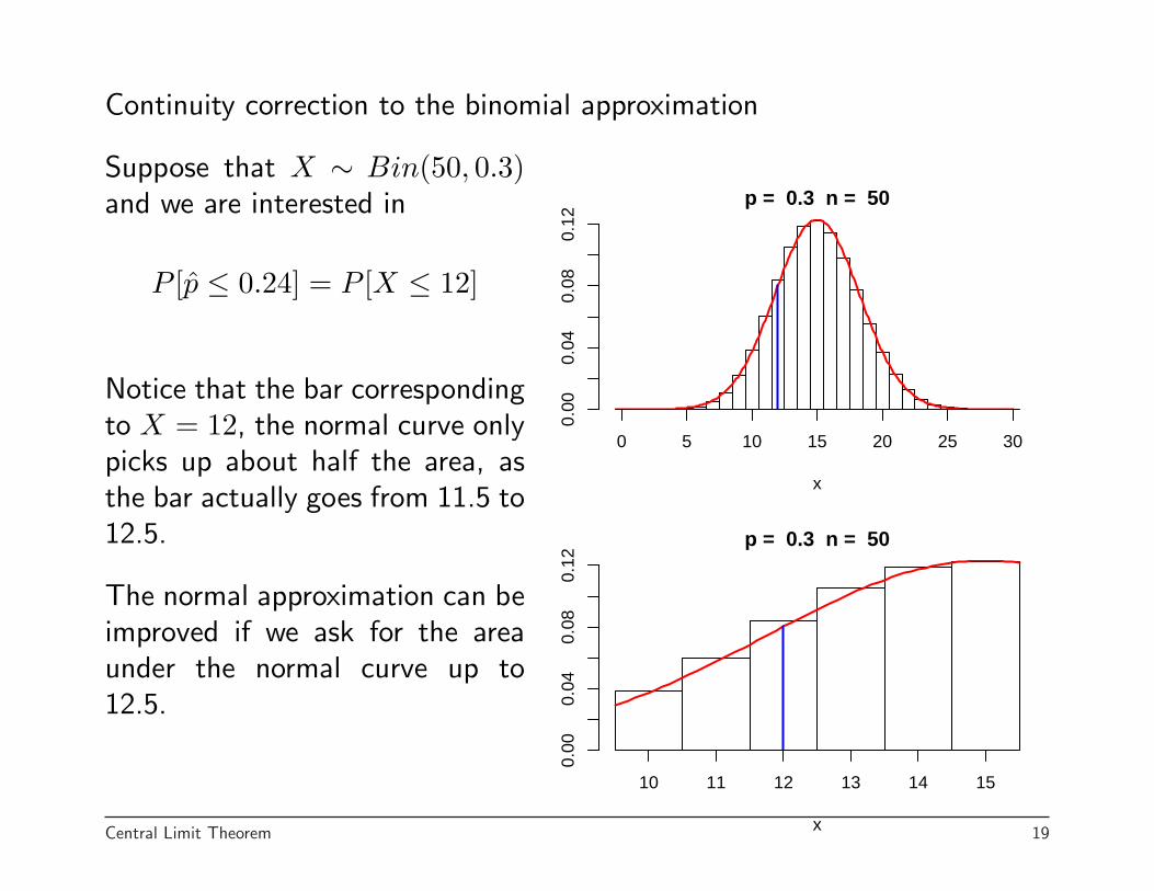
Continuity correction to the binomial approximation

p = 0.3 n = 50

x

0.00

0.04

0.08

0.12

0 5 10 15 20 25 30

p = 0.3 n = 50

x

0.00

0.04

0.08

0.12

10 11 12 13 14 15

Suppose that X ∼ Bin(50, 0.3)and we are interested in

P [p̂ ≤ 0.24] = P [X ≤ 12]

Notice that the bar correspondingto X = 12, the normal curve onlypicks up about half the area, asthe bar actually goes from 11.5 to12.5.

The normal approximation can beimproved if we ask for the areaunder the normal curve up to12.5.

Central Limit Theorem 19

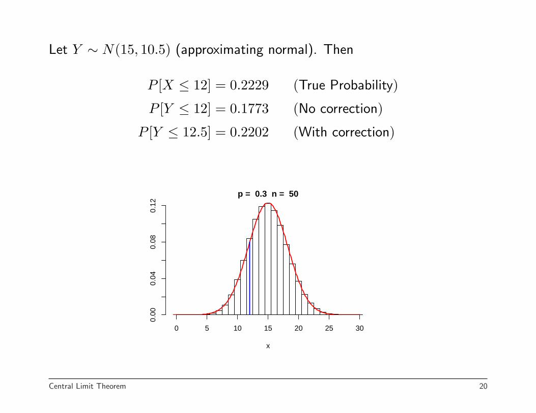
Let Y ∼ N(15, 10.5) (approximating normal). Then

P [X ≤ 12] = 0.2229 (True Probability)

P [Y ≤ 12] = 0.1773 (No correction)

P [Y ≤ 12.5] = 0.2202 (With correction)

p = 0.3 n = 50

x

0.00

0.04

0.08

0.12

0 5 10 15 20 25 30

Central Limit Theorem 20

While this does give a better answer for many problems, normally Irecommend ignoring it. If the correction makes a difference, you probablywant to be doing an exact probability calculation instead.

When will the CLT work better?

• Big n

• Distribution of Xi close to normal. Approximation holds exactly if n = 1if Xi ∼ N(µ, σ2).

• Xi roughly symmetric. As we observed with the binomial examples, thecloser p was to 0.5, thus closer to symmetry, the better the approximationworks. The more skewness there is in the distribution of the observations,the bigger n needs to be.

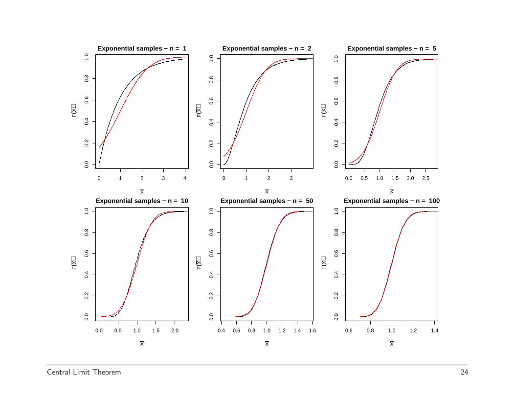
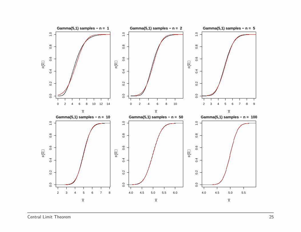
In the following plots, the histogram represents 10,000 simulated X̄s, theblack curves are the true densities or CDFs, and the red curves are thenormal approximations.

Central Limit Theorem 21

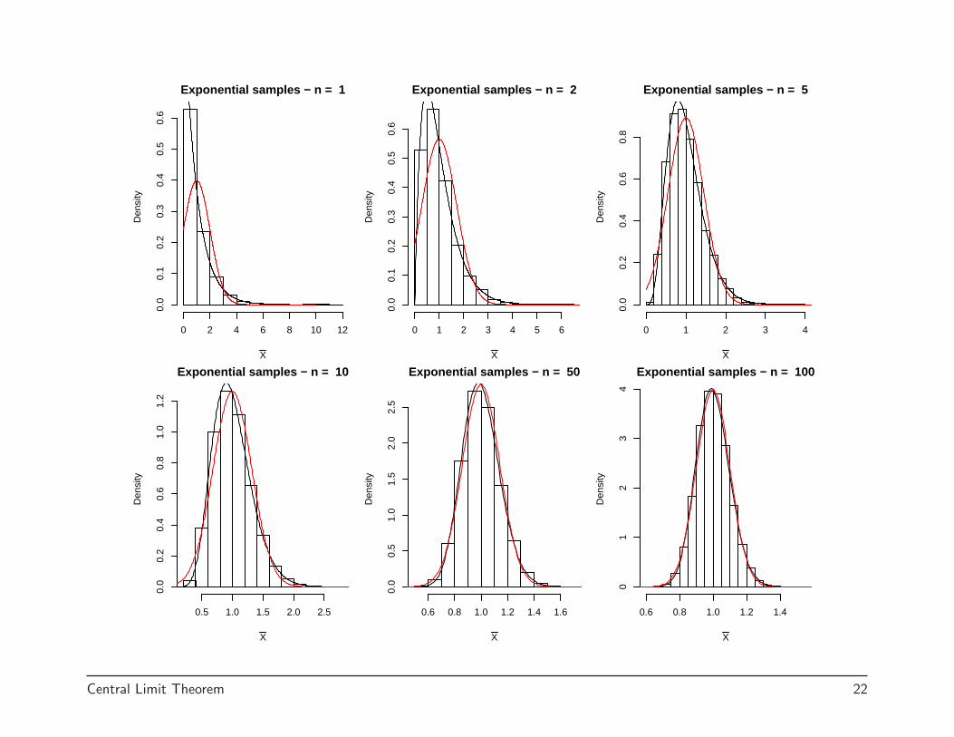
Exponential samples − n = 1

X

Den

sity

0 2 4 6 8 10 12

0.0

0.1

0.2

0.3

0.4

0.5

0.6

Exponential samples − n = 2

XD

ensi

ty

0 1 2 3 4 5 6

0.0

0.1

0.2

0.3

0.4

0.5

0.6

Exponential samples − n = 5

X

Den

sity

0 1 2 3 4

0.0

0.2

0.4

0.6

0.8

Exponential samples − n = 10

X

Den

sity

0.5 1.0 1.5 2.0 2.5

0.0

0.2

0.4

0.6

0.8

1.0

1.2

Exponential samples − n = 50

X

Den

sity

0.6 0.8 1.0 1.2 1.4 1.6

0.0

0.5

1.0

1.5

2.0

2.5

Exponential samples − n = 100

X

Den

sity

0.6 0.8 1.0 1.2 1.40

12

34

Central Limit Theorem 22

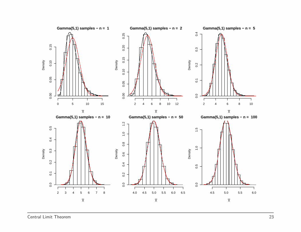
Gamma(5,1) samples − n = 1

X

Den

sity

0 5 10 15

0.00

0.05

0.10

0.15

Gamma(5,1) samples − n = 2

XD

ensi

ty

2 4 6 8 10 12

0.00

0.05

0.10

0.15

0.20

0.25

Gamma(5,1) samples − n = 5

X

Den

sity

2 4 6 8 10

0.0

0.1

0.2

0.3

0.4

Gamma(5,1) samples − n = 10

X

Den

sity

2 3 4 5 6 7 8

0.0

0.1

0.2

0.3

0.4

0.5

Gamma(5,1) samples − n = 50

X

Den

sity

4.0 4.5 5.0 5.5 6.0 6.5

0.0

0.2

0.4

0.6

0.8

1.0

1.2

Gamma(5,1) samples − n = 100

X

Den

sity

4.5 5.0 5.5 6.00.

00.

51.

01.

5

Central Limit Theorem 23

0 1 2 3 4

0.0

0.2

0.4

0.6

0.8

1.0

Exponential samples − n = 1

X

F(X

)

0 1 2 3

0.0

0.2

0.4

0.6

0.8

1.0

Exponential samples − n = 2

XF(X

)

0.0 0.5 1.0 1.5 2.0 2.5

0.0

0.2

0.4

0.6

0.8

1.0

Exponential samples − n = 5

X

F(X

)0.0 0.5 1.0 1.5 2.0

0.0

0.2

0.4

0.6

0.8

1.0

Exponential samples − n = 10

X

F(X

)

0.4 0.6 0.8 1.0 1.2 1.4 1.6

0.0

0.2

0.4

0.6

0.8

1.0

Exponential samples − n = 50

X

F(X

)

0.6 0.8 1.0 1.2 1.40.

00.

20.

40.

60.

81.

0

Exponential samples − n = 100

X

F(X

)

Central Limit Theorem 24

0 2 4 6 8 10 12 14

0.0

0.2

0.4

0.6

0.8

1.0

Gamma(5,1) samples − n = 1

X

F(X

)

0 2 4 6 8 10

0.0

0.2

0.4

0.6

0.8

1.0

Gamma(5,1) samples − n = 2

XF(X

)

2 3 4 5 6 7 8 9

0.0

0.2

0.4

0.6

0.8

1.0

Gamma(5,1) samples − n = 5

X

F(X

)2 3 4 5 6 7 8

0.0

0.2

0.4

0.6

0.8

1.0

Gamma(5,1) samples − n = 10

X

F(X

)

4.0 4.5 5.0 5.5 6.0

0.0

0.2

0.4

0.6

0.8

1.0

Gamma(5,1) samples − n = 50

X

F(X

)

4.0 4.5 5.0 5.50.

00.

20.

40.

60.

81.

0

Gamma(5,1) samples − n = 100

X

F(X

)

Central Limit Theorem 25

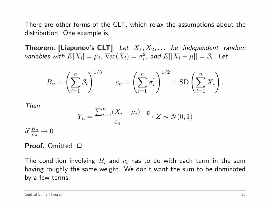
There are other forms of the CLT, which relax the assumptions about thedistribution. One example is,

Theorem. [Liapunov’s CLT] Let X1, X2, . . . be independent randomvariables with E[Xi] = µi, Var(Xi) = σ2

i , and E[|Xi − µ|] = βi. Let

Bn =

(n∑

i=1

βi

)1/3

cn =

(n∑

i=1

σ2i

)1/2

= SD

(n∑

i=1

Xi

).

Then

Yn =∑n

i=1(Xi − µi)cn

D−→ Z ∼ N(0, 1)

if Bncn→ 0

Proof. Omitted 2

The condition involving Bi and ci has to do with each term in the sumhaving roughly the same weight. We don’t want the sum to be dominatedby a few terms.

Central Limit Theorem 26

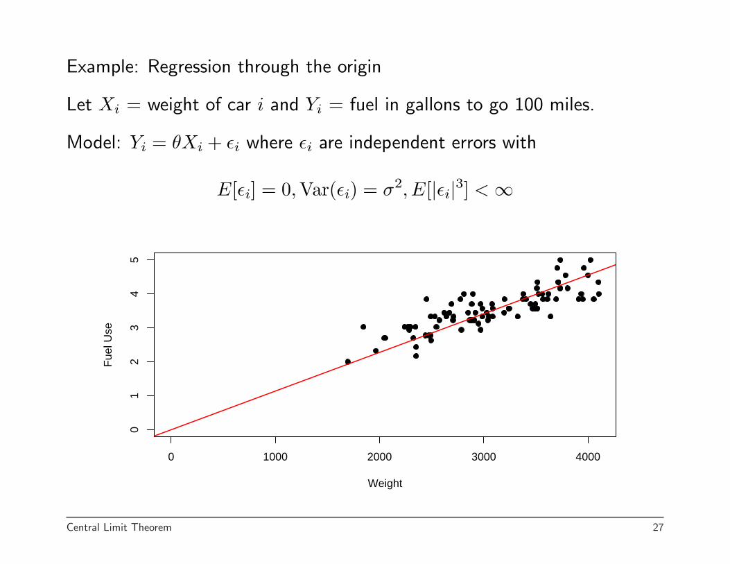
Example: Regression through the origin

Let Xi = weight of car i and Yi = fuel in gallons to go 100 miles.

Model: Yi = θXi + εi where εi are independent errors with

E[εi] = 0, Var(εi) = σ2, E[|εi|3] < ∞

0 1000 2000 3000 4000

01

23

45

Weight

Fue

l Use

Central Limit Theorem 27

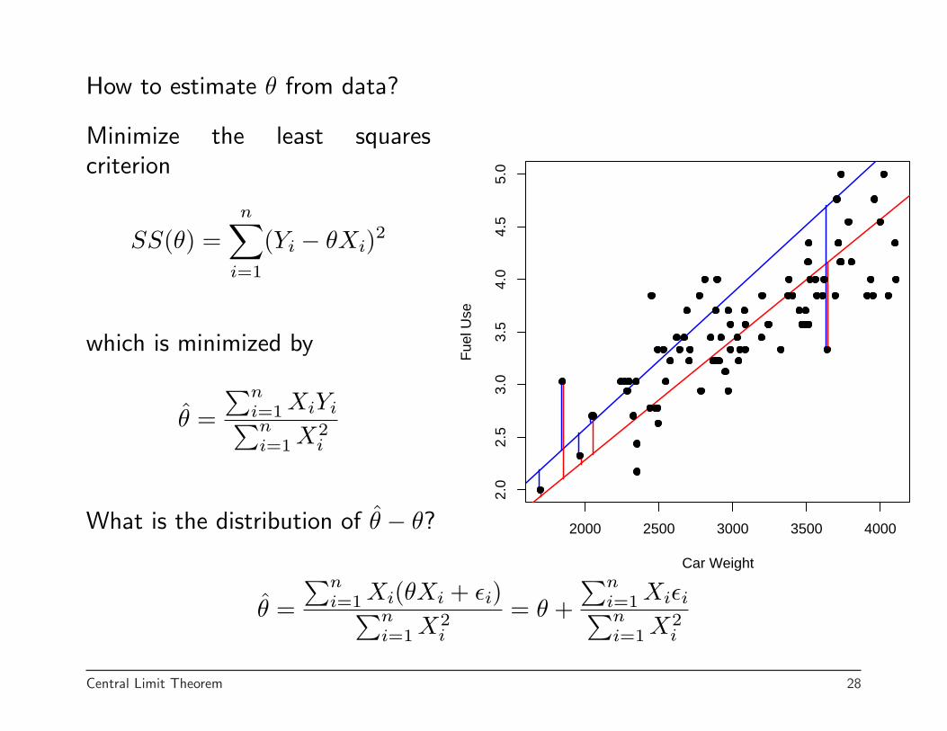
How to estimate θ from data?

2000 2500 3000 3500 4000

2.0

2.5

3.0

3.5

4.0

4.5

5.0

Car Weight

Fue

l Use

Minimize the least squarescriterion

SS(θ) =n∑

i=1

(Yi − θXi)2

which is minimized by

θ̂ =∑n

i=1 XiYi∑ni=1 X2

i

What is the distribution of θ̂ − θ?

θ̂ =∑n

i=1 Xi(θXi + εi)∑ni=1 X2

i

= θ +∑n

i=1 Xiεi∑ni=1 X2

i

Central Limit Theorem 28

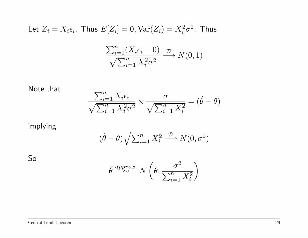
Let Zi = Xiεi. Thus E[Zi] = 0, Var(Zi) = X2i σ2. Thus

∑ni=1(Xiεi − 0)√∑n

i=1 X2i σ2

D−→ N(0, 1)

Note that ∑ni=1 Xiεi√∑ni=1 X2

i σ2× σ√∑n

i=1 X2i

= (θ̂ − θ)

implying

(θ̂ − θ)√∑n

i=1 X2i

D−→ N(0, σ2)

So

θ̂approx.∼ N

(θ,

σ2

∑ni=1 X2

i

)

Central Limit Theorem 29

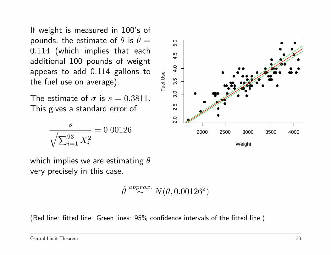
2000 2500 3000 3500 4000

2.0

2.5

3.0

3.5

4.0

4.5

5.0

Weight

Fue

l Use

If weight is measured in 100’s ofpounds, the estimate of θ is θ̂ =0.114 (which implies that eachadditional 100 pounds of weightappears to add 0.114 gallons tothe fuel use on average).

The estimate of σ is s = 0.3811.This gives a standard error of

s√∑93i=1 X2

i

= 0.00126

which implies we are estimating θvery precisely in this case.

θ̂approx.∼ N(θ, 0.001262)

(Red line: fitted line. Green lines: 95% confidence intervals of the fitted line.)

Central Limit Theorem 30

There are also versions of the CLT that allow the variables to have limitedlevels of dependency.

They all have the basic form (under different technical conditions)

Sn − E[Sn]SD(Sn)

D−→ N(0, 1) orX̄n − E[X̄n]

SD(X̄n)D−→ N(0, 1)

which imply

Snapprox.∼ N(E[Sn], Var(Sn)) or X̄n

approx.∼ N(E[X̄n], Var(X̄n))

Central Limit Theorem 31

These mathematical results suggest why the normal distribution is socommonly seen with real data.

They say, that when an effect is the sum of a large number of small,roughly equally weighted terms, the effect should be approximately normallydistributed.

For example, peoples heights are influenced by (a potentially) large numberof genes and by various environmental effects.

Histograms of adult men and women’s heights are both well described bynormal densities.

Central Limit Theorem 32

Theorem. [Slutsky’s Theorems] Suppose XnD−→ X and Yn

P−→ c(constant). Then

1. Xn + YnD−→ X + c

2. XnYnD−→ cX

3. If c 6= 0, XnYn

D−→ Xnc

4. Let f(x, y) be a continuous function. Then f(Xn, Yn) D−→ f(X, c)

Example: Suppose X1, X2, . . . are iid with E[Xi] = µ, Var(Xi) = σ2. Whatare the distributions of the t-statistics

Tn =X̄n − µ

Sn/√

n

as n →∞.

Central Limit Theorem 33

As we have seen before

1. By the central limit theorem

X̄n − µ

σ/√

n

D−→ N(0, 1)

2. S2n

P−→ σ2, or Snσ

P−→ 1

T =[X̄n − µ

σ/√

n

]/Sn

σ

D−→ N(0, 1)1

= N(0, 1)

This result proves that the tn distributions converge to the N(0, 1)distribution.

Central Limit Theorem 34