Control-Flow Graphs &

Dataflow Analysis CS4410: Spring 2013

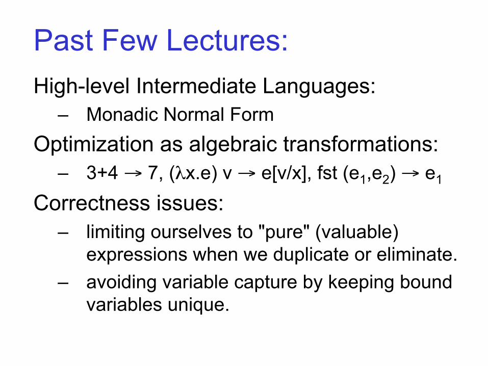
Past Few Lectures: High-level Intermediate Languages:

–  Monadic Normal Form Optimization as algebraic transformations:

–  3+4 → 7, (λx.e) v → e[v/x], fst (e1,e2) → e1 Correctness issues:

–  limiting ourselves to "pure" (valuable) expressions when we duplicate or eliminate.

–  avoiding variable capture by keeping bound variables unique.

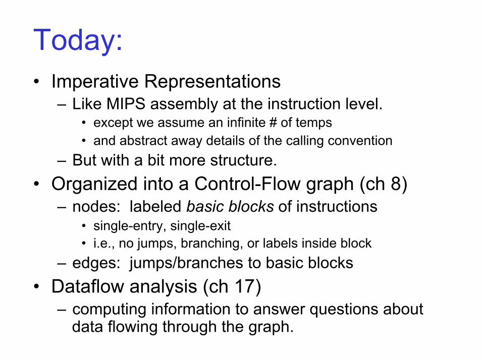
Today: •  Imperative Representations

–  Like MIPS assembly at the instruction level. •  except we assume an infinite # of temps •  and abstract away details of the calling convention

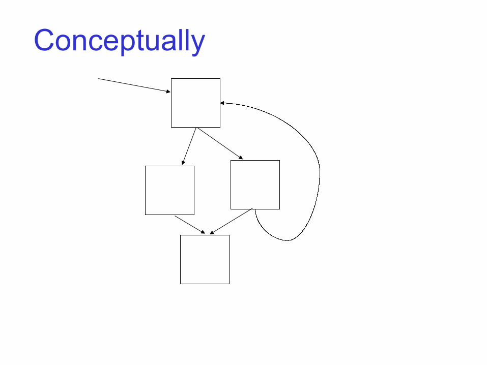
–  But with a bit more structure. •  Organized into a Control-Flow graph (ch 8)

–  nodes: labeled basic blocks of instructions •  single-entry, single-exit •  i.e., no jumps, branching, or labels inside block

–  edges: jumps/branches to basic blocks •  Dataflow analysis (ch 17)

–  computing information to answer questions about data flowing through the graph.

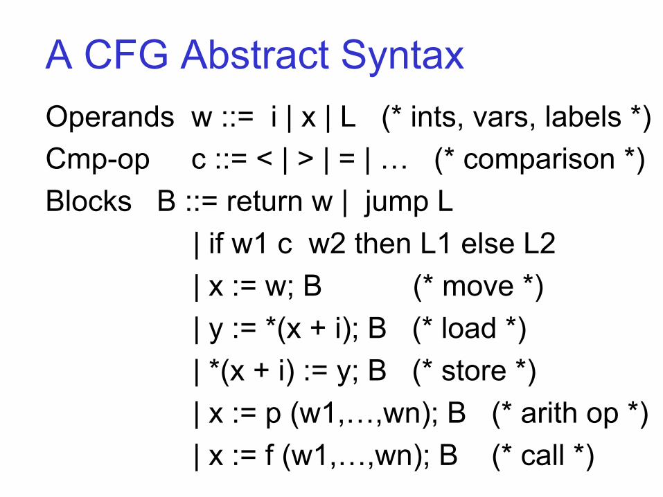
A CFG Abstract Syntax Operands w ::= i | x | L (* ints, vars, labels *) Cmp-op c ::= < | > | = | … (* comparison *) Blocks B ::= return w | jump L | if w1 c w2 then L1 else L2 | x := w; B (* move *) | y := *(x + i); B (* load *) | *(x + i) := y; B (* store *) | x := p (w1,…,wn); B (* arith op *) | x := f (w1,…,wn); B (* call *)

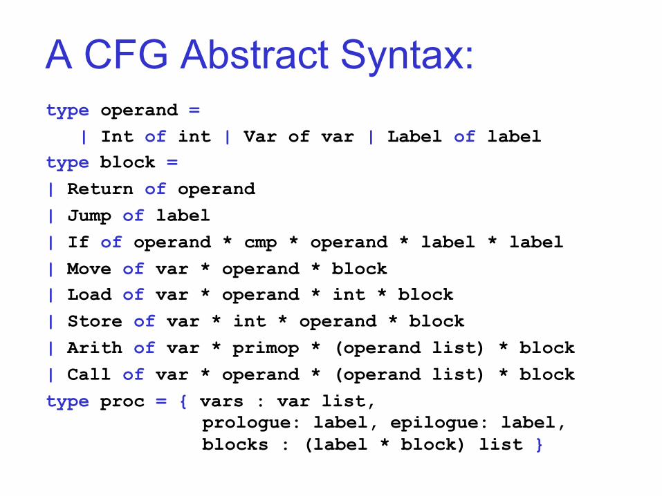
A CFG Abstract Syntax: type operand = | Int of int | Var of var | Label of label type block = | Return of operand | Jump of label | If of operand * cmp * operand * label * label | Move of var * operand * block | Load of var * operand * int * block | Store of var * int * operand * block | Arith of var * primop * (operand list) * block | Call of var * operand * (operand list) * block type proc = { vars : var list,

prologue: label, epilogue: label, blocks : (label * block) list }

Conceptually

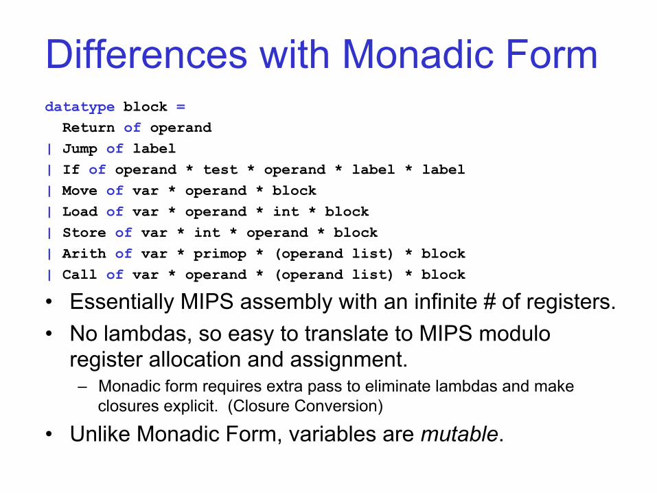
Differences with Monadic Form datatype block = Return of operand | Jump of label | If of operand * test * operand * label * label | Move of var * operand * block | Load of var * operand * int * block | Store of var * int * operand * block | Arith of var * primop * (operand list) * block | Call of var * operand * (operand list) * block

•  Essentially MIPS assembly with an infinite # of registers. •  No lambdas, so easy to translate to MIPS modulo

register allocation and assignment. –  Monadic form requires extra pass to eliminate lambdas and make

closures explicit. (Closure Conversion)

•  Unlike Monadic Form, variables are mutable.

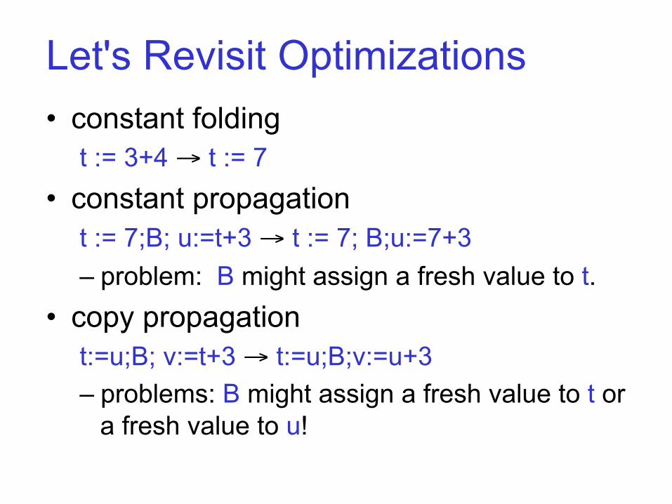
Let's Revisit Optimizations •  constant folding

t := 3+4 → t := 7 •  constant propagation

t := 7;B; u:=t+3 → t := 7; B;u:=7+3 – problem: B might assign a fresh value to t.

•  copy propagation t:=u;B; v:=t+3 → t:=u;B;v:=u+3 – problems: B might assign a fresh value to t or

a fresh value to u!

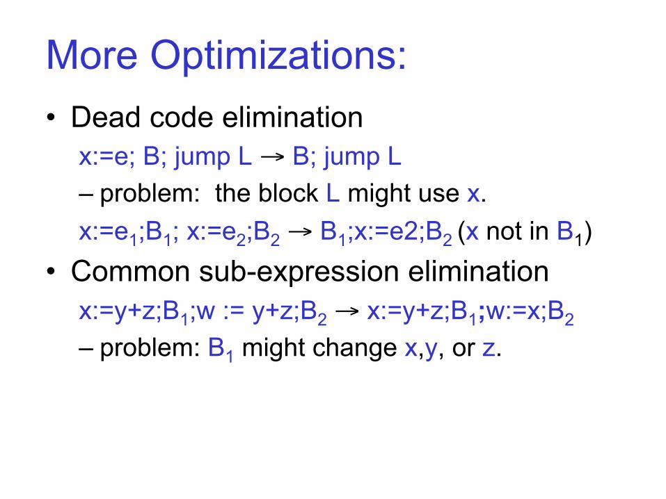
More Optimizations: •  Dead code elimination

x:=e; B; jump L → B; jump L – problem: the block L might use x. x:=e1;B1; x:=e2;B2 → B1;x:=e2;B2 (x not in B1)

•  Common sub-expression elimination x:=y+z;B1;w := y+z;B2 → x:=y+z;B1;w:=x;B2 – problem: B1 might change x,y, or z.

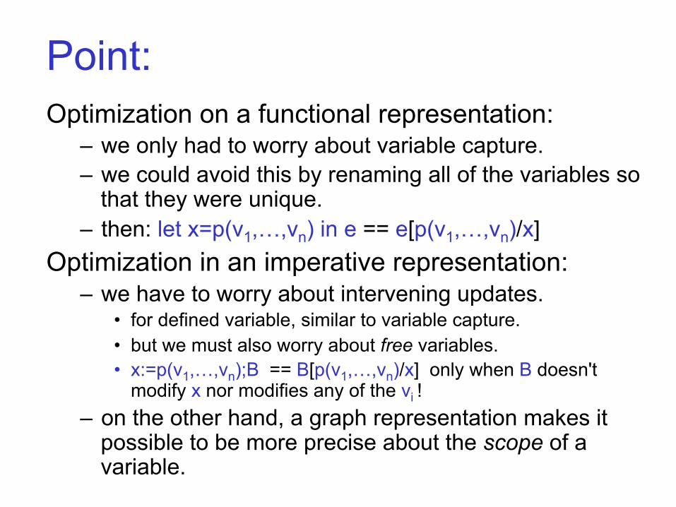
Point: Optimization on a functional representation:

–  we only had to worry about variable capture. –  we could avoid this by renaming all of the variables so

that they were unique. –  then: let x=p(v1,…,vn) in e == e[p(v1,…,vn)/x]

Optimization in an imperative representation: –  we have to worry about intervening updates.

•  for defined variable, similar to variable capture. •  but we must also worry about free variables. •  x:=p(v1,…,vn);B == B[p(v1,…,vn)/x] only when B doesn't

modify x nor modifies any of the vi ! –  on the other hand, a graph representation makes it

possible to be more precise about the scope of a variable.

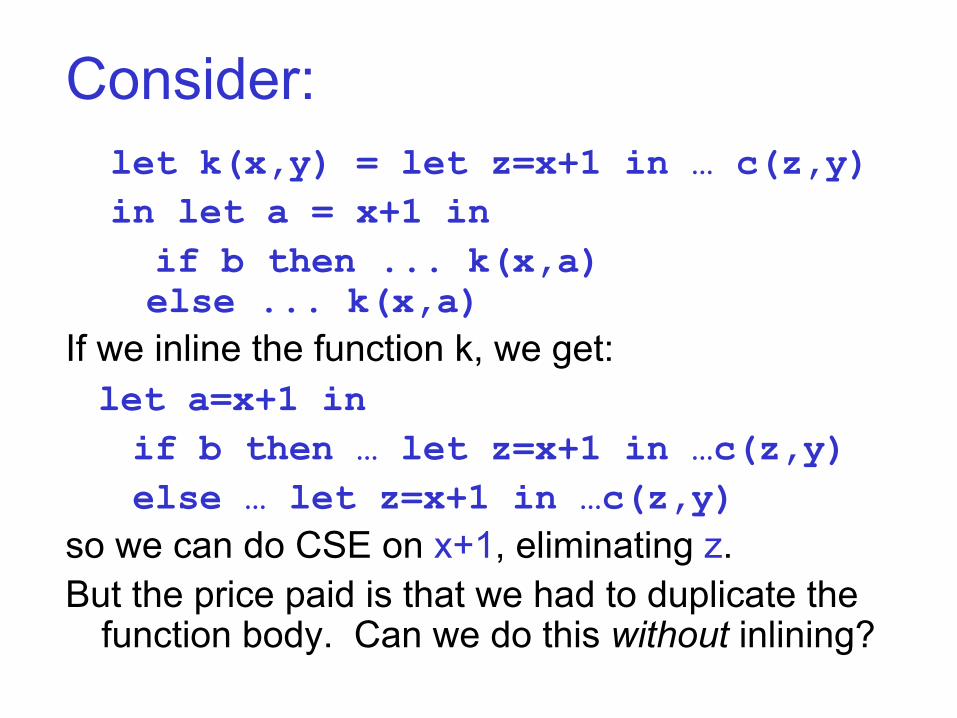
Consider: let k(x,y) = let z=x+1 in … c(z,y) in let a = x+1 in if b then ... k(x,a) else ... k(x,a)

If we inline the function k, we get: let a=x+1 in if b then … let z=x+1 in …c(z,y) else … let z=x+1 in …c(z,y) so we can do CSE on x+1, eliminating z. But the price paid is that we had to duplicate the

function body. Can we do this without inlining?

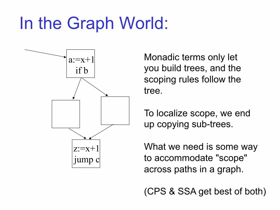
In the Graph World:

a:=x+1 if b

z:=x+1 jump c

Monadic terms only let you build trees, and the scoping rules follow the tree. To localize scope, we end up copying sub-trees. What we need is some way to accommodate "scope" across paths in a graph. (CPS & SSA get best of both)

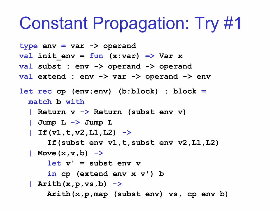
Constant Propagation: Try #1 type env = var -> operand val init_env = fun (x:var) => Var x val subst : env -> operand -> operand val extend : env -> var -> operand -> env let rec cp (env:env) (b:block) : block = match b with | Return v -> Return (subst env v) | Jump L -> Jump L | If(v1,t,v2,L1,L2) -> If(subst env v1,t,subst env v2,L1,L2) | Move(x,v,b) -> let v' = subst env v in cp (extend env x v') b | Arith(x,p,vs,b) -> Arith(x,p,map (subst env) vs, cp env b)

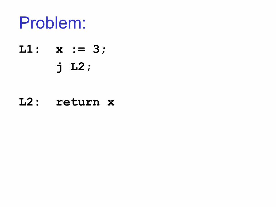
Problem: L1: x := 3; j L2; L2: return x

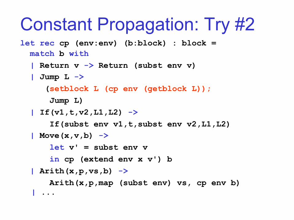
Constant Propagation: Try #2 let rec cp (env:env) (b:block) : block = match b with | Return v -> Return (subst env v) | Jump L -> (setblock L (cp env (getblock L)); Jump L) | If(v1,t,v2,L1,L2) -> If(subst env v1,t,subst env v2,L1,L2) | Move(x,v,b) -> let v' = subst env v in cp (extend env x v') b | Arith(x,p,vs,b) -> Arith(x,p,map (subst env) vs, cp env b)

| ...

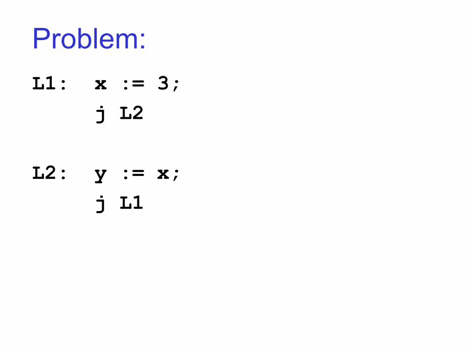
Problem: L1: x := 3; j L2 L2: y := x; j L1

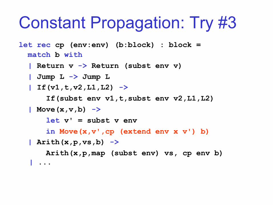
Constant Propagation: Try #3 let rec cp (env:env) (b:block) : block = match b with | Return v -> Return (subst env v) | Jump L -> Jump L | If(v1,t,v2,L1,L2) -> If(subst env v1,t,subst env v2,L1,L2) | Move(x,v,b) -> let v' = subst v env in Move(x,v',cp (extend env x v') b) | Arith(x,p,vs,b) -> Arith(x,p,map (subst env) vs, cp env b)

| ...

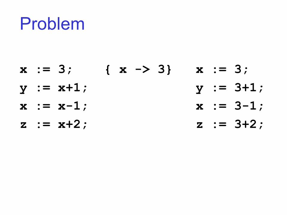
Problem x := 3; { x -> 3} x := 3; y := x+1; y := 3+1; x := x-1; x := 3-1; z := x+2; z := 3+2;

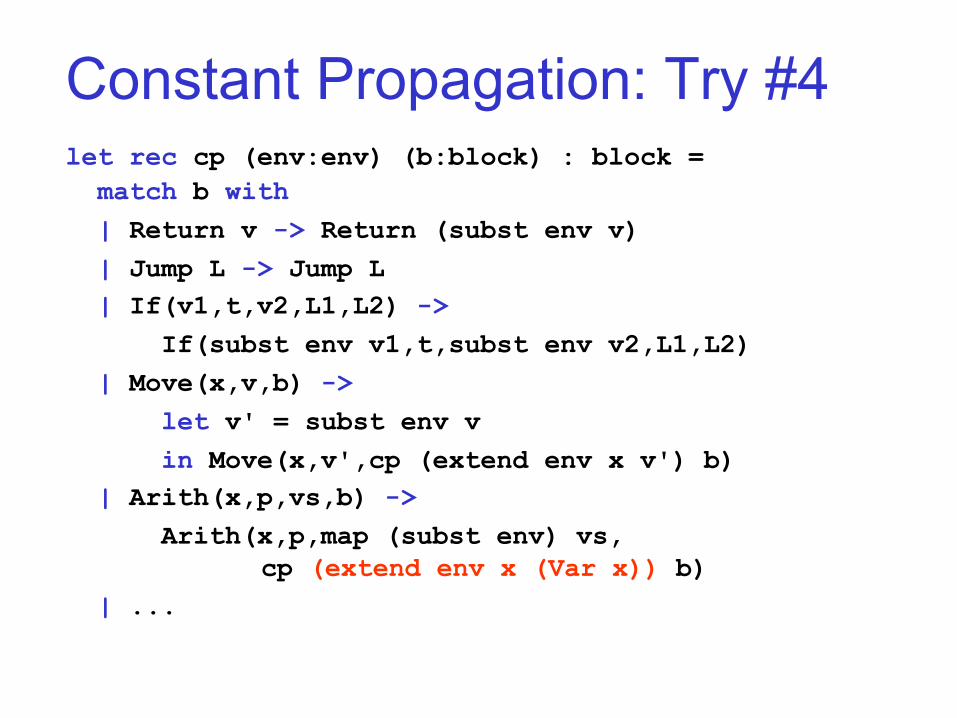
Constant Propagation: Try #4 let rec cp (env:env) (b:block) : block = match b with | Return v -> Return (subst env v) | Jump L -> Jump L | If(v1,t,v2,L1,L2) -> If(subst env v1,t,subst env v2,L1,L2) | Move(x,v,b) -> let v' = subst env v in Move(x,v',cp (extend env x v') b) | Arith(x,p,vs,b) -> Arith(x,p,map (subst env) vs,

cp (extend env x (Var x)) b) | ...

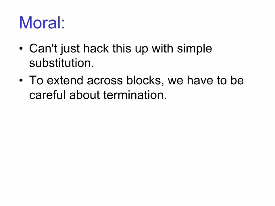
Moral: •  Can't just hack this up with simple

substitution. •  To extend across blocks, we have to be

careful about termination.

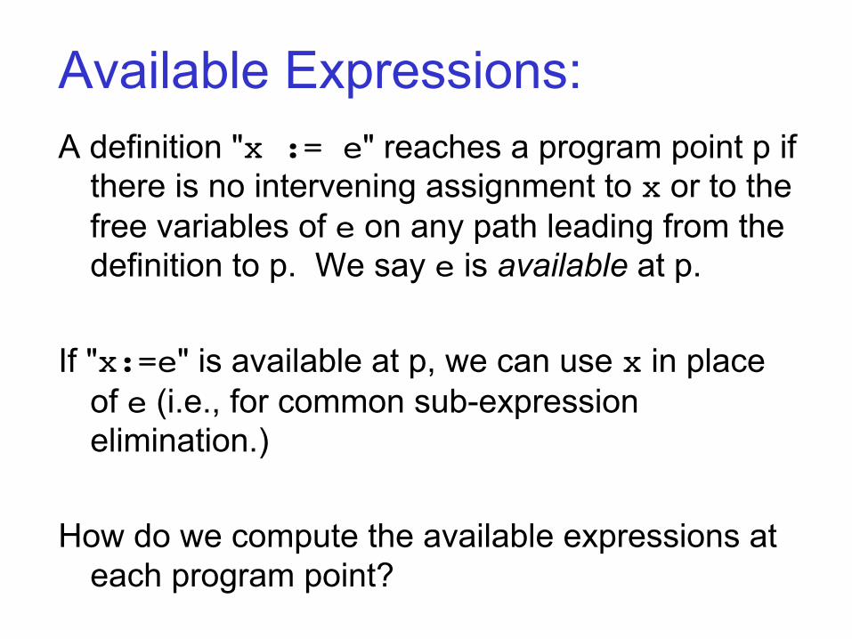
Available Expressions: A definition "x := e" reaches a program point p if

there is no intervening assignment to x or to the free variables of e on any path leading from the definition to p. We say e is available at p.

If "x:=e" is available at p, we can use x in place

of e (i.e., for common sub-expression elimination.)

How do we compute the available expressions at

each program point?

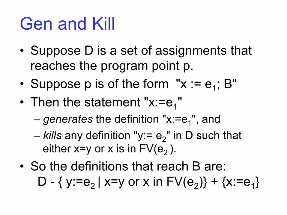
Gen and Kill •  Suppose D is a set of assignments that

reaches the program point p. •  Suppose p is of the form "x := e1; B" •  Then the statement "x:=e1"

– generates the definition "x:=e1", and – kills any definition "y:= e2" in D such that

either x=y or x is in FV(e2 ). •  So the definitions that reach B are:

D - { y:=e2 | x=y or x in FV(e2)} + {x:=e1}

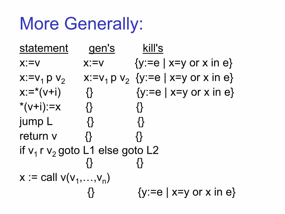
More Generally: statement gen's kill's x:=v x:=v {y:=e | x=y or x in e} x:=v1 p v2 x:=v1 p v2 {y:=e | x=y or x in e} x:=*(v+i) {} {y:=e | x=y or x in e} *(v+i):=x {} {} jump L {} {} return v {} {} if v1 r v2 goto L1 else goto L2

{} {} x := call v(v1,…,vn) {} {y:=e | x=y or x in e}

Flowing through the Graph: •  Given the available expressions Din[L] that flow

into a block labeled L, we can compute the definitions Dout[L] that flow out by just using the gen & kill's for each statement in L's block.

•  For each block L, we can define: –  succ[L] = the blocks L might jump to. –  pred[L] = the blocks that might jump to L.

•  We can then flow Dout[L] to all of the blocks in succ[L].

•  They'll compute new Dout's and flow them to their successors and so on.

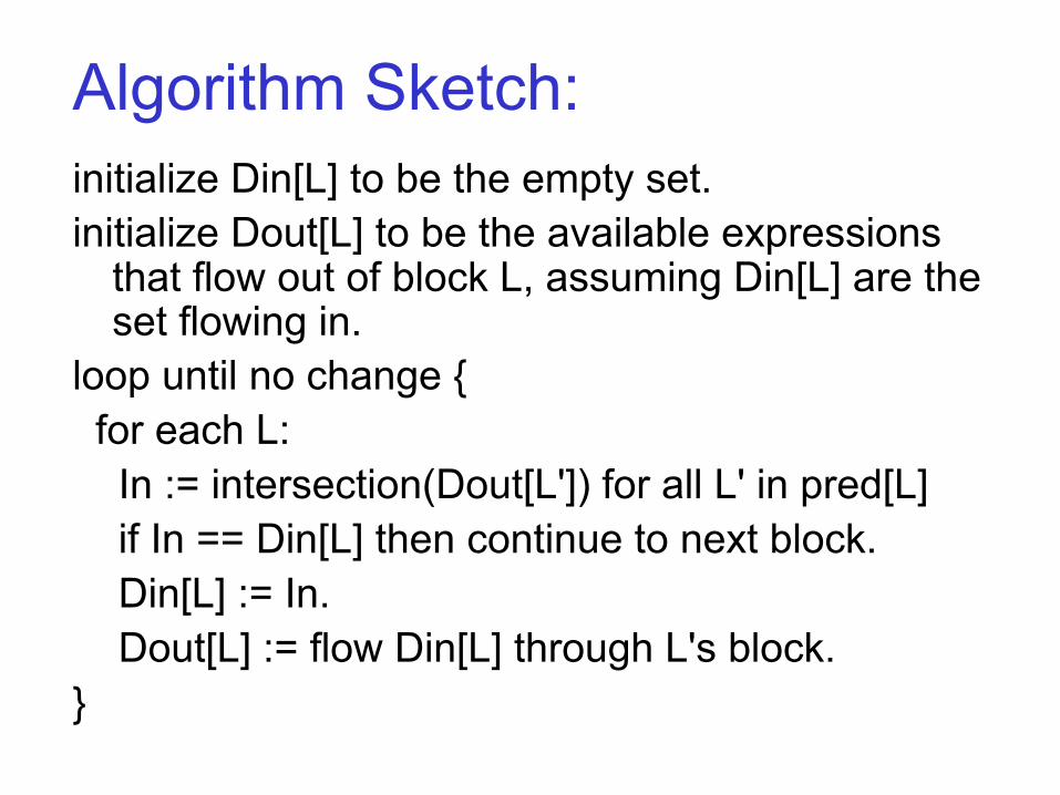
Algorithm Sketch: initialize Din[L] to be the empty set. initialize Dout[L] to be the available expressions

that flow out of block L, assuming Din[L] are the set flowing in.

loop until no change { for each L: In := intersection(Dout[L']) for all L' in pred[L] if In == Din[L] then continue to next block. Din[L] := In. Dout[L] := flow Din[L] through L's block. }

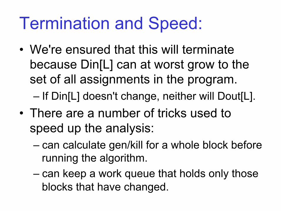
Termination and Speed: •  We're ensured that this will terminate

because Din[L] can at worst grow to the set of all assignments in the program. –  If Din[L] doesn't change, neither will Dout[L].

•  There are a number of tricks used to speed up the analysis: – can calculate gen/kill for a whole block before

running the algorithm. – can keep a work queue that holds only those

blocks that have changed.

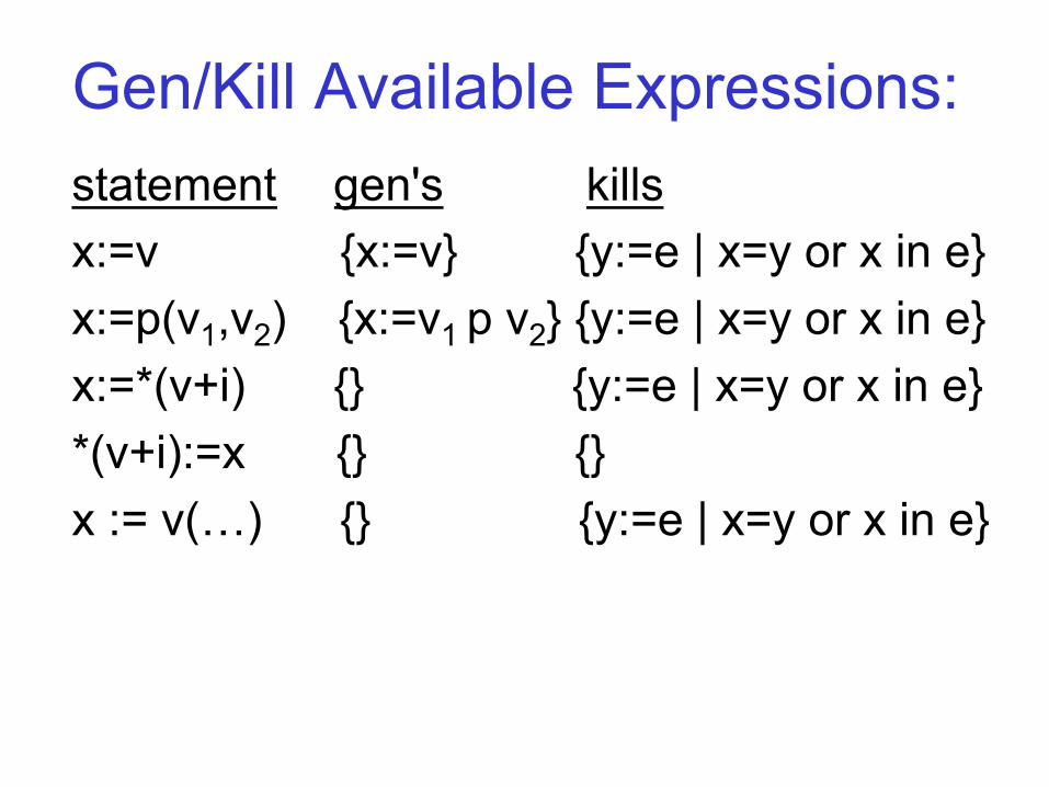
Gen/Kill Available Expressions: statement gen's kills x:=v {x:=v} {y:=e | x=y or x in e} x:=p(v1,v2) {x:=v1 p v2} {y:=e | x=y or x in e} x:=*(v+i) {} {y:=e | x=y or x in e} *(v+i):=x {} {} x := v(…) {} {y:=e | x=y or x in e}

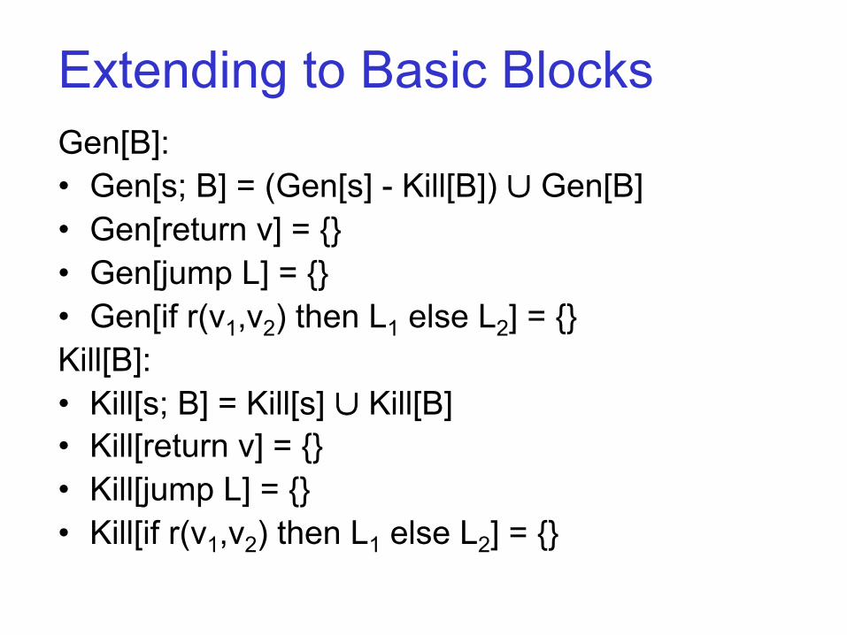
Extending to Basic Blocks Gen[B]: •  Gen[s; B] = (Gen[s] - Kill[B]) ∪ Gen[B] •  Gen[return v] = {} •  Gen[jump L] = {} •  Gen[if r(v1,v2) then L1 else L2] = {} Kill[B]: •  Kill[s; B] = Kill[s] ∪ Kill[B] •  Kill[return v] = {} •  Kill[jump L] = {} •  Kill[if r(v1,v2) then L1 else L2] = {}

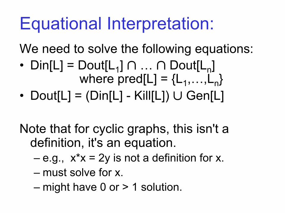
Equational Interpretation: We need to solve the following equations: •  Din[L] = Dout[L1] ∩ … ∩ Dout[Ln]

where pred[L] = {L1,…,Ln} •  Dout[L] = (Din[L] - Kill[L]) ∪ Gen[L]

Note that for cyclic graphs, this isn't a definition, it's an equation. – e.g., x*x = 2y is not a definition for x. – must solve for x. – might have 0 or > 1 solution.

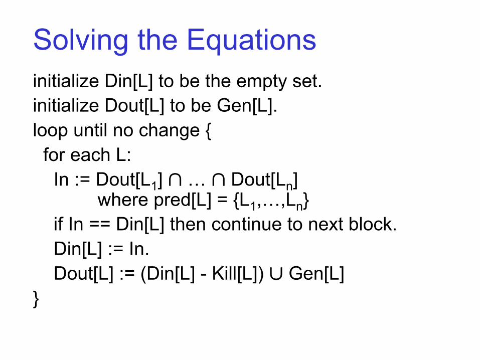
Solving the Equations initialize Din[L] to be the empty set. initialize Dout[L] to be Gen[L]. loop until no change { for each L: In := Dout[L1] ∩ … ∩ Dout[Ln]

where pred[L] = {L1,…,Ln} if In == Din[L] then continue to next block. Din[L] := In. Dout[L] := (Din[L] - Kill[L]) ∪ Gen[L] }

Recap: Control-flow graphs:

–  nodes are basic blocks •  single-entry, single-exit sequences of code •  statements are imperative •  variables have no nested scope

–  edges correspond to jumps/branches Dataflow analysis:

–  Example: available expressions –  Iterative solution

Next: Another dataflow analysis - Liveness

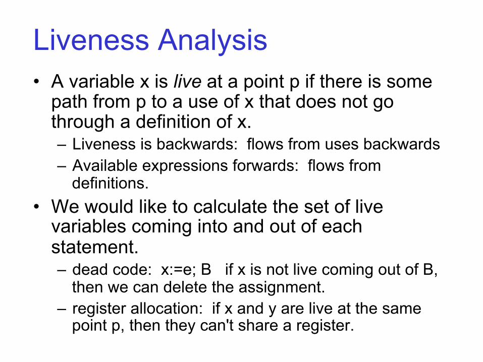
Liveness Analysis •  A variable x is live at a point p if there is some

path from p to a use of x that does not go through a definition of x. –  Liveness is backwards: flows from uses backwards –  Available expressions forwards: flows from

definitions. •  We would like to calculate the set of live

variables coming into and out of each statement. –  dead code: x:=e; B if x is not live coming out of B,

then we can delete the assignment. –  register allocation: if x and y are live at the same

point p, then they can't share a register.

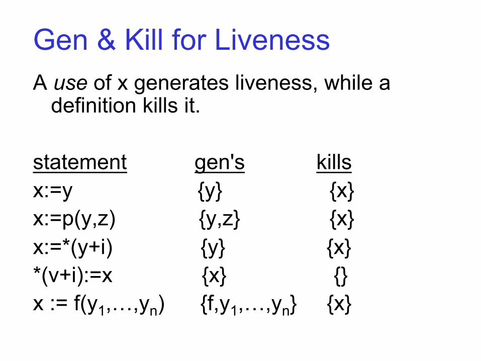
Gen & Kill for Liveness A use of x generates liveness, while a

definition kills it. statement gen's kills x:=y {y} {x} x:=p(y,z) {y,z} {x} x:=*(y+i) {y} {x} *(v+i):=x {x} {} x := f(y1,…,yn) {f,y1,…,yn} {x}

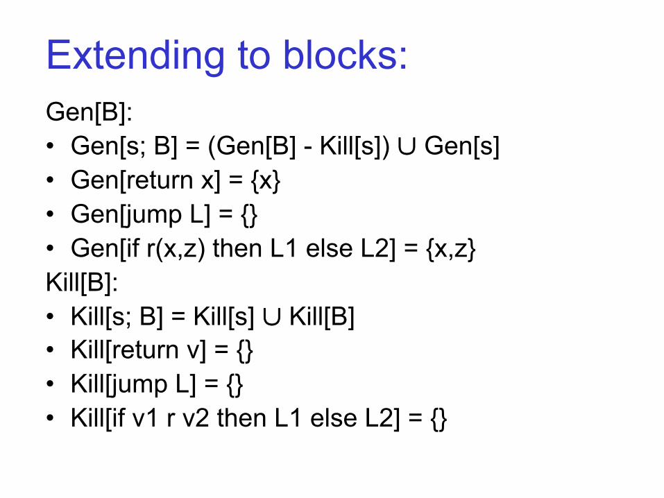
Extending to blocks: Gen[B]: •  Gen[s; B] = (Gen[B] - Kill[s]) ∪ Gen[s] •  Gen[return x] = {x} •  Gen[jump L] = {} •  Gen[if r(x,z) then L1 else L2] = {x,z} Kill[B]: •  Kill[s; B] = Kill[s] ∪ Kill[B] •  Kill[return v] = {} •  Kill[jump L] = {} •  Kill[if v1 r v2 then L1 else L2] = {}

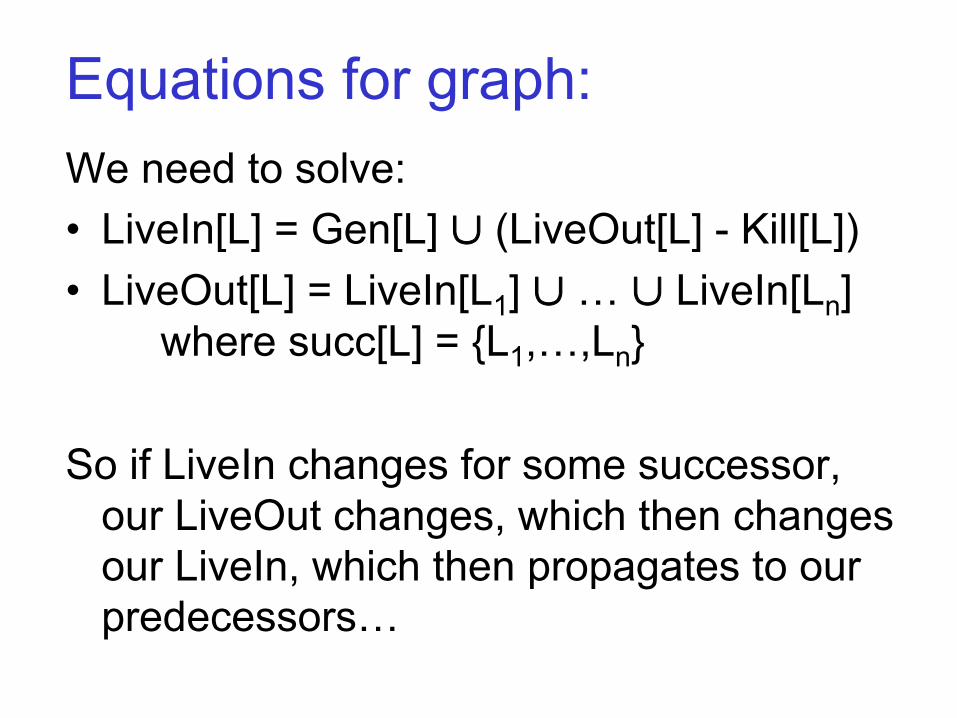
Equations for graph: We need to solve: •  LiveIn[L] = Gen[L] ∪ (LiveOut[L] - Kill[L]) •  LiveOut[L] = LiveIn[L1] ∪ … ∪ LiveIn[Ln]

where succ[L] = {L1,…,Ln}

So if LiveIn changes for some successor, our LiveOut changes, which then changes our LiveIn, which then propagates to our predecessors…

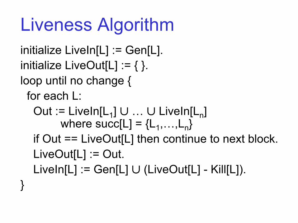
Liveness Algorithm initialize LiveIn[L] := Gen[L]. initialize LiveOut[L] := { }. loop until no change { for each L: Out := LiveIn[L1] ∪ … ∪ LiveIn[Ln]

where succ[L] = {L1,…,Ln} if Out == LiveOut[L] then continue to next block. LiveOut[L] := Out. LiveIn[L] := Gen[L] ∪ (LiveOut[L] - Kill[L]). }

Speeding up the Analysis •  For liveness, flow is backwards.

–  so processing successors before predecessors will avoid doing another loop.

–  of course, when there's a loop, we have to just pick a place to break the cycle.

•  For available expressions, flow is forwards. –  so processing predecessors before successors will

avoid doing another loop. •  Only need to revisit blocks that change.

–  keep a priority queue, sorted by flow order

Representing Sets (See Appel) •  Consider liveness analysis:

–  need to calculate sets of variables. –  need efficient union, subtraction.

•  Usual solution uses bitsets –  use bitwise operations (e.g., &, |, ~, etc.) to

implement set operations. –  note: this solution scales well, but has bad

asymptotic complexity compared to a sparse representation.

•  Complexity of whole liveness algorithm? –  worst case, O(n4) assuming set ops are O(n) –  in practice it's roughly quadratic.

Coming up… •  Register allocation [ch. 11]

– seen first part: liveness analysis – next: construct interference graph –  then: graph coloring & simplification

•  Loop-oriented optimizations [ch. 18] – e.g., loop-invariant removal

•  CPS & SSA