Continuous age-structured models

p. 1

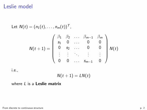
Leslie model

Let N(t) = (n1(t), . . . , nm(t))T ,

N(t + 1) =

β1 β2 . . . βm−1 βms1 0 . . . 0 00 s2 . . . 0 0...

.... . .

......

0 0 . . . sm−1 0

N(t)

i.e.,N(t + 1) = LN(t)

where L is a Leslie matrix

From discrete to continuous structure p. 2

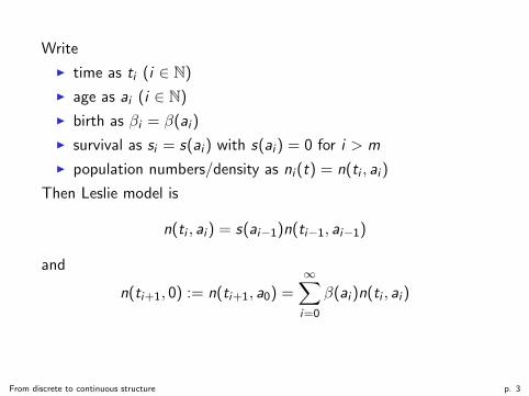
Write

I time as ti (i ∈ N)

I age as ai (i ∈ N)

I birth as βi = β(ai )

I survival as si = s(ai ) with s(ai ) = 0 for i > m

I population numbers/density as ni (t) = n(ti , ai )

Then Leslie model is

n(ti , ai ) = s(ai−1)n(ti−1, ai−1)

and

n(ti+1, 0) := n(ti+1, a0) =∞∑i=0

β(ai )n(ti , ai )

From discrete to continuous structure p. 3

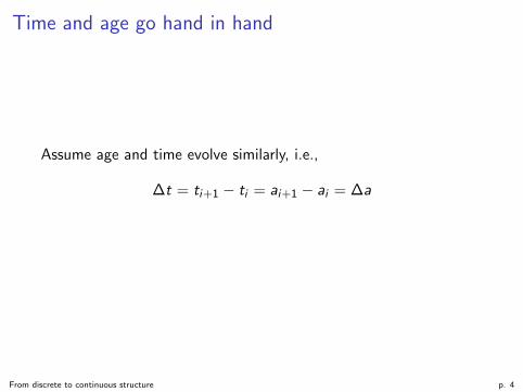
Time and age go hand in hand

Assume age and time evolve similarly, i.e.,

∆t = ti+1 − ti = ai+1 − ai = ∆a

From discrete to continuous structure p. 4

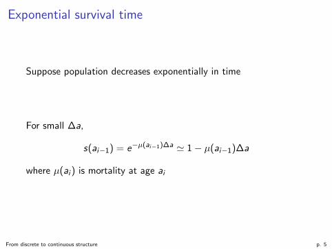
Exponential survival time

Suppose population decreases exponentially in time

For small ∆a,

s(ai−1) = e−µ(ai−1)∆a ' 1− µ(ai−1)∆a

where µ(ai ) is mortality at age ai

From discrete to continuous structure p. 5

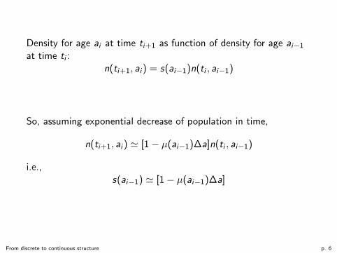
Density for age ai at time ti+1 as function of density for age ai−1

at time ti :n(ti+1, ai ) = s(ai−1)n(ti , ai−1)

So, assuming exponential decrease of population in time,

n(ti+1, ai ) ' [1− µ(ai−1)∆a]n(ti , ai−1)

i.e.,s(ai−1) ' [1− µ(ai−1)∆a]

From discrete to continuous structure p. 6

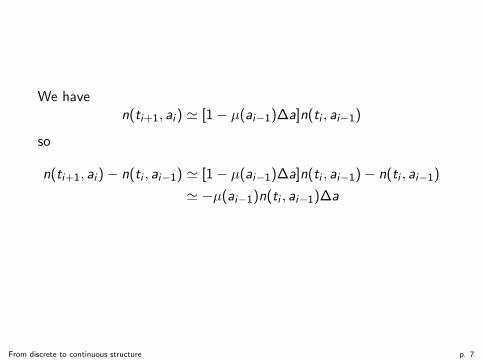
We haven(ti+1, ai ) ' [1− µ(ai−1)∆a]n(ti , ai−1)

so

n(ti+1, ai )− n(ti , ai−1) ' [1− µ(ai−1)∆a]n(ti , ai−1)− n(ti , ai−1)

' −µ(ai−1)n(ti , ai−1)∆a

From discrete to continuous structure p. 7

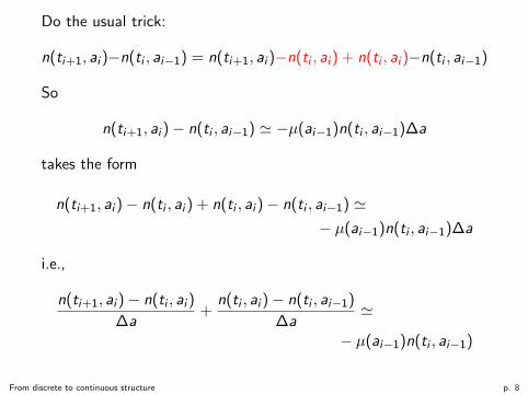
Do the usual trick:

n(ti+1, ai )−n(ti , ai−1) = n(ti+1, ai )−n(ti , ai ) + n(ti , ai )−n(ti , ai−1)

So

n(ti+1, ai )− n(ti , ai−1) ' −µ(ai−1)n(ti , ai−1)∆a

takes the form

n(ti+1, ai )− n(ti , ai ) + n(ti , ai )− n(ti , ai−1) '− µ(ai−1)n(ti , ai−1)∆a

i.e.,

n(ti+1, ai )− n(ti , ai )

∆a+

n(ti , ai )− n(ti , ai−1)

∆a'

− µ(ai−1)n(ti , ai−1)

From discrete to continuous structure p. 8

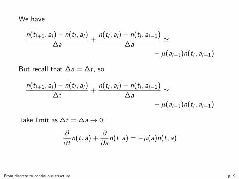
We have

n(ti+1, ai )− n(ti , ai )

∆a+

n(ti , ai )− n(ti , ai−1)

∆a'

− µ(ai−1)n(ti , ai−1)

But recall that ∆a = ∆t, so

n(ti+1, ai )− n(ti , ai )

∆t+

n(ti , ai )− n(ti , ai−1)

∆a'

− µ(ai−1)n(ti , ai−1)

Take limit as ∆t = ∆a→ 0:

∂

∂tn(t, a) +

∂

∂an(t, a) = −µ(a)n(t, a)

From discrete to continuous structure p. 9

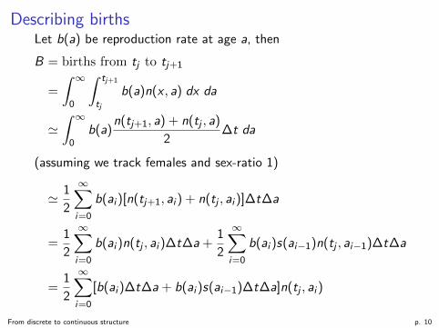
Describing birthsLet b(a) be reproduction rate at age a, then

B = births from tj to tj+1

=

∫ ∞0

∫ tj+1

tj

b(a)n(x , a) dx da

'∫ ∞

0b(a)

n(tj+1, a) + n(tj , a)

2∆t da

(assuming we track females and sex-ratio 1)

' 1

2

∞∑i=0

b(ai )[n(tj+1, ai ) + n(tj , ai )]∆t∆a

=1

2

∞∑i=0

b(ai )n(tj , ai )∆t∆a +1

2

∞∑i=0

b(ai )s(ai−1)n(tj , ai−1)∆t∆a

=1

2

∞∑i=0

[b(ai )∆t∆a + b(ai )s(ai−1)∆t∆a]n(tj , ai )

From discrete to continuous structure p. 10

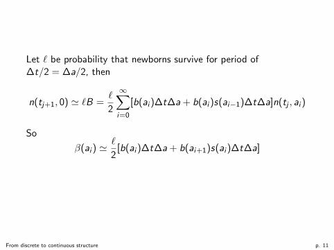
Let ` be probability that newborns survive for period of∆t/2 = ∆a/2, then

n(tj+1, 0) ' `B =`

2

∞∑i=0

[b(ai )∆t∆a + b(ai )s(ai−1)∆t∆a]n(tj , ai )

So

β(ai ) '`

2[b(ai )∆t∆a + b(ai+1)s(ai )∆t∆a]

From discrete to continuous structure p. 11

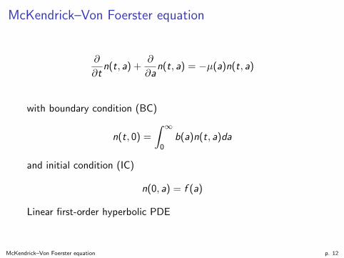
McKendrick–Von Foerster equation

∂

∂tn(t, a) +

∂

∂an(t, a) = −µ(a)n(t, a)

with boundary condition (BC)

n(t, 0) =

∫ ∞0

b(a)n(t, a)da

and initial condition (IC)

n(0, a) = f (a)

Linear first-order hyperbolic PDE

McKendrick–Von Foerster equation p. 12

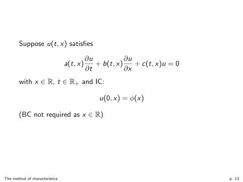
Suppose u(t, x) satisfies

a(t, x)∂u

∂t+ b(t, x)

∂u

∂x+ c(t, x)u = 0

with x ∈ R, t ∈ R+ and IC:

u(0, x) = φ(x)

(BC not required as x ∈ R)

The method of characteristics p. 13

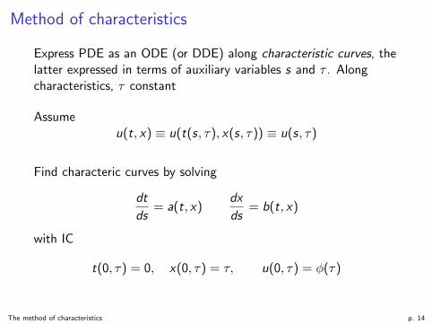
Method of characteristics

Express PDE as an ODE (or DDE) along characteristic curves, thelatter expressed in terms of auxiliary variables s and τ . Alongcharacteristics, τ constant

Assumeu(t, x) ≡ u(t(s, τ), x(s, τ)) ≡ u(s, τ)

Find characteric curves by solving

dt

ds= a(t, x)

dx

ds= b(t, x)

with IC

t(0, τ) = 0, x(0, τ) = τ, u(0, τ) = φ(τ)

The method of characteristics p. 14

t(0, τ) = 0, x(0, τ) = τ, u(0, τ) = φ(τ)

t

x

The method of characteristics p. 15

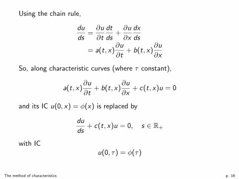
Using the chain rule,

du

ds=∂u

∂t

dt

ds+∂u

∂x

dx

ds

= a(t, x)∂u

∂t+ b(t, x)

∂u

∂x

So, along characteristic curves (where τ constant),

a(t, x)∂u

∂t+ b(t, x)

∂u

∂x+ c(t, x)u = 0

and its IC u(0, x) = φ(x) is replaced by

du

ds+ c(t, x)u = 0, s ∈ R+

with ICu(0, τ) = φ(τ)

The method of characteristics p. 16

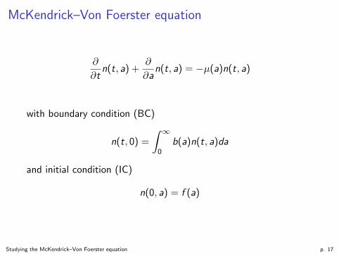
McKendrick–Von Foerster equation

∂

∂tn(t, a) +

∂

∂an(t, a) = −µ(a)n(t, a)

with boundary condition (BC)

n(t, 0) =

∫ ∞0

b(a)n(t, a)da

and initial condition (IC)

n(0, a) = f (a)

Studying the McKendrick–Von Foerster equation p. 17

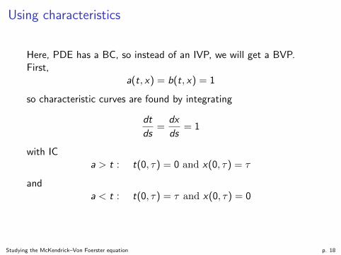
Using characteristics

Here, PDE has a BC, so instead of an IVP, we will get a BVP.First,

a(t, x) = b(t, x) = 1

so characteristic curves are found by integrating

dt

ds=

dx

ds= 1

with ICa > t : t(0, τ) = 0 and x(0, τ) = τ

anda < t : t(0, τ) = τ and x(0, τ) = 0

Studying the McKendrick–Von Foerster equation p. 18

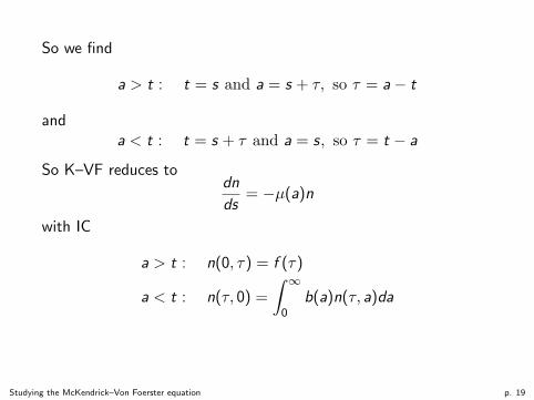
So we find

a > t : t = s and a = s + τ, so τ = a− t

anda < t : t = s + τ and a = s, so τ = t − a

So K–VF reduces todn

ds= −µ(a)n

with IC

a > t : n(0, τ) = f (τ)

a < t : n(τ, 0) =

∫ ∞0

b(a)n(τ, a)da

Studying the McKendrick–Von Foerster equation p. 19

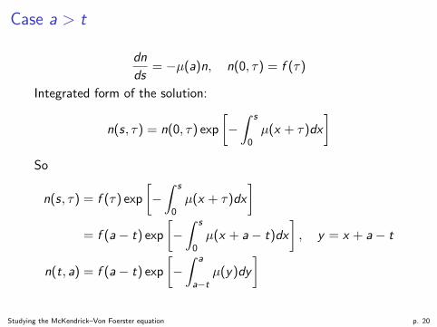
Case a > t

dn

ds= −µ(a)n, n(0, τ) = f (τ)

Integrated form of the solution:

n(s, τ) = n(0, τ) exp

[−∫ s

0µ(x + τ)dx

]So

n(s, τ) = f (τ) exp

[−∫ s

0µ(x + τ)dx

]= f (a− t) exp

[−∫ s

0µ(x + a− t)dx

], y = x + a− t

n(t, a) = f (a− t) exp

[−∫ a

a−tµ(y)dy

]

Studying the McKendrick–Von Foerster equation p. 20

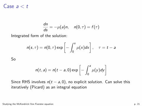
Case a < t

dn

ds= −µ(a)n, n(0, τ) = f (τ)

Integrated form of the solution:

n(s, τ) = n(0, τ) exp

[−∫ s

0µ(x)dx

], τ = t − a

So

n(t, a) = n(t − a, 0) exp

[−∫ a

0µ(y)dy

]Since RHS involves n(t − a, 0), no explicit solution. Can solve thisiteratively (Picard) as an integral equation

Studying the McKendrick–Von Foerster equation p. 21

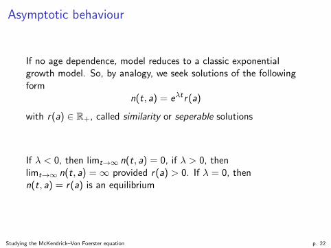
Asymptotic behaviour

If no age dependence, model reduces to a classic exponentialgrowth model. So, by analogy, we seek solutions of the followingform

n(t, a) = eλtr(a)

with r(a) ∈ R+, called similarity or seperable solutions

If λ < 0, then limt→∞ n(t, a) = 0, if λ > 0, thenlimt→∞ n(t, a) =∞ provided r(a) > 0. If λ = 0, thenn(t, a) = r(a) is an equilibrium

Studying the McKendrick–Von Foerster equation p. 22

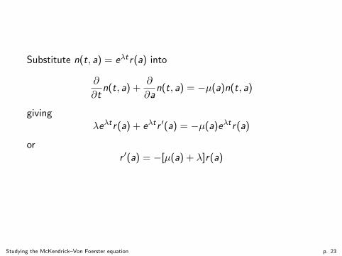
Substitute n(t, a) = eλtr(a) into

∂

∂tn(t, a) +

∂

∂an(t, a) = −µ(a)n(t, a)

givingλeλtr(a) + eλtr ′(a) = −µ(a)eλtr(a)

orr ′(a) = −[µ(a) + λ]r(a)

Studying the McKendrick–Von Foerster equation p. 23

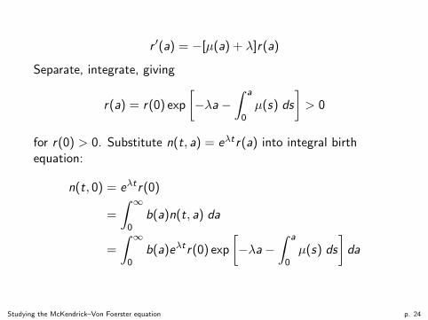
r ′(a) = −[µ(a) + λ]r(a)

Separate, integrate, giving

r(a) = r(0) exp

[−λa−

∫ a

0µ(s) ds

]> 0

for r(0) > 0. Substitute n(t, a) = eλtr(a) into integral birthequation:

n(t, 0) = eλtr(0)

=

∫ ∞0

b(a)n(t, a) da

=

∫ ∞0

b(a)eλtr(0) exp

[−λa−

∫ a

0µ(s) ds

]da

Studying the McKendrick–Von Foerster equation p. 24

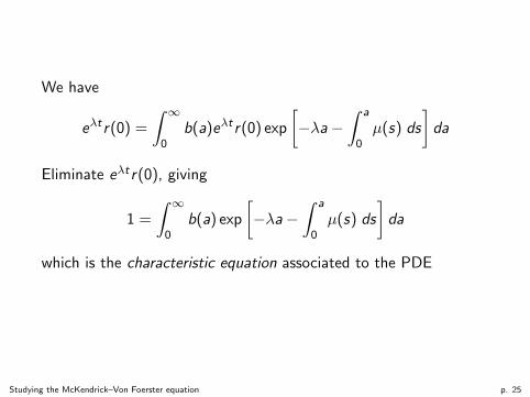
We have

eλtr(0) =

∫ ∞0

b(a)eλtr(0) exp

[−λa−

∫ a

0µ(s) ds

]da

Eliminate eλtr(0), giving

1 =

∫ ∞0

b(a) exp

[−λa−

∫ a

0µ(s) ds

]da

which is the characteristic equation associated to the PDE

Studying the McKendrick–Von Foerster equation p. 25

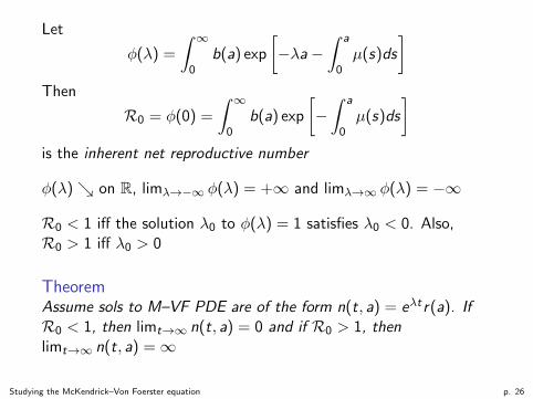
Let

φ(λ) =

∫ ∞0

b(a) exp

[−λa−

∫ a

0µ(s)ds

]Then

R0 = φ(0) =

∫ ∞0

b(a) exp

[−∫ a

0µ(s)ds

]is the inherent net reproductive number

φ(λ)↘ on R, limλ→−∞ φ(λ) = +∞ and limλ→∞ φ(λ) = −∞

R0 < 1 iff the solution λ0 to φ(λ) = 1 satisfies λ0 < 0. Also,R0 > 1 iff λ0 > 0

TheoremAssume sols to M–VF PDE are of the form n(t, a) = eλtr(a). IfR0 < 1, then limt→∞ n(t, a) = 0 and if R0 > 1, thenlimt→∞ n(t, a) =∞

Studying the McKendrick–Von Foerster equation p. 26