
Continuing Work in Robust Portfolio Optimizationdano/talks/w.pdfContinuing Work in Robust Portfolio...
127
Continuing Work in Robust Portfolio Optimization Daniel Bienstock Columbia University, New York 30 June 2008 Daniel Bienstock ( Columbia University, New York) Continuing Work in Robust Portfolio Optimization 30 June 2008 1 / 58
Transcript of Continuing Work in Robust Portfolio Optimizationdano/talks/w.pdfContinuing Work in Robust Portfolio...

Continuing Work in Robust PortfolioOptimization
Daniel Bienstock
Columbia University, New York
30 June 2008
Daniel Bienstock ( Columbia University, New York)Continuing Work in Robust Portfolio Optimization 30 June 2008 1 / 58
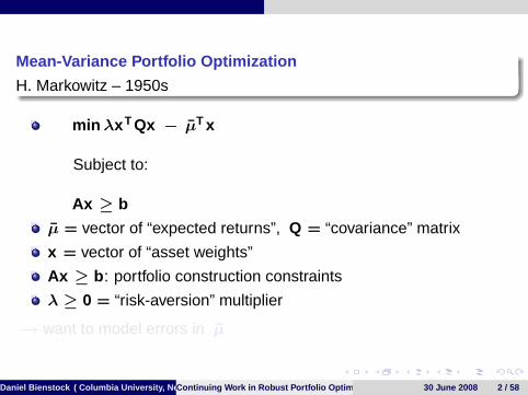
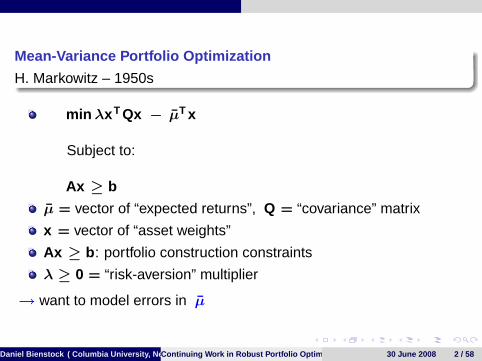
Mean-Variance Portfolio Optimization
H. Markowitz – 1950s
min λx T Qx − µT x
Subject to:
Ax ≥ b
µ = vector of “expected returns”, Q = “covariance” matrix
x = vector of “asset weights”
Ax ≥ b : portfolio construction constraints
λ ≥ 0 = “risk-aversion” multiplier
→ want to model errors in µ
Daniel Bienstock ( Columbia University, New York)Continuing Work in Robust Portfolio Optimization 30 June 2008 2 / 58
Robust Optimization
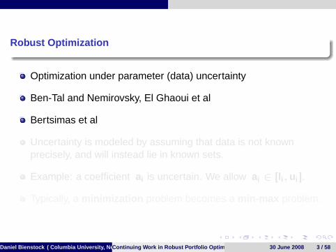
Optimization under parameter (data) uncertainty
Ben-Tal and Nemirovsky, El Ghaoui et al
Bertsimas et al
Uncertainty is modeled by assuming that data is not knownprecisely, and will instead lie in known sets.
Example: a coefficient ai is uncertain. We allow ai ∈ [l i , u i ].
Typically, a minimization problem becomes a min-max problem.
Daniel Bienstock ( Columbia University, New York)Continuing Work in Robust Portfolio Optimization 30 June 2008 3 / 58
Robust Optimization
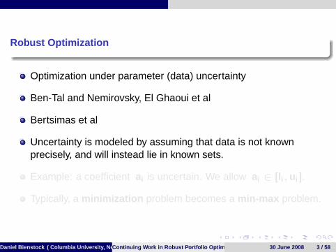
Optimization under parameter (data) uncertainty
Ben-Tal and Nemirovsky, El Ghaoui et al
Bertsimas et al
Uncertainty is modeled by assuming that data is not knownprecisely, and will instead lie in known sets.
Example: a coefficient ai is uncertain. We allow ai ∈ [l i , u i ].
Typically, a minimization problem becomes a min-max problem.
Daniel Bienstock ( Columbia University, New York)Continuing Work in Robust Portfolio Optimization 30 June 2008 3 / 58
Robust Optimization
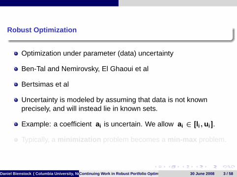
Optimization under parameter (data) uncertainty
Ben-Tal and Nemirovsky, El Ghaoui et al
Bertsimas et al
Uncertainty is modeled by assuming that data is not knownprecisely, and will instead lie in known sets.
Example: a coefficient ai is uncertain. We allow ai ∈ [l i , u i ].
Typically, a minimization problem becomes a min-max problem.
Daniel Bienstock ( Columbia University, New York)Continuing Work in Robust Portfolio Optimization 30 June 2008 3 / 58
Robust Optimization
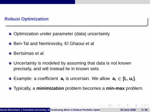
Optimization under parameter (data) uncertainty
Ben-Tal and Nemirovsky, El Ghaoui et al
Bertsimas et al
Uncertainty is modeled by assuming that data is not knownprecisely, and will instead lie in known sets.
Example: a coefficient ai is uncertain. We allow ai ∈ [l i , u i ].
Typically, a minimization problem becomes a min-max problem.
Daniel Bienstock ( Columbia University, New York)Continuing Work in Robust Portfolio Optimization 30 June 2008 3 / 58
Robust Optimization
Optimization under parameter (data) uncertainty
Ben-Tal and Nemirovsky, El Ghaoui et al
Bertsimas et al
Uncertainty is modeled by assuming that data is not knownprecisely, and will instead lie in known sets.
Example: a coefficient ai is uncertain. We allow ai ∈ [l i , u i ].
Typically, a minimization problem becomes a min-max problem.
Daniel Bienstock ( Columbia University, New York)Continuing Work in Robust Portfolio Optimization 30 June 2008 3 / 58
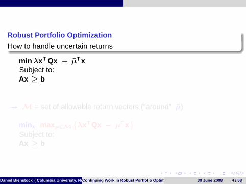
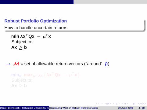
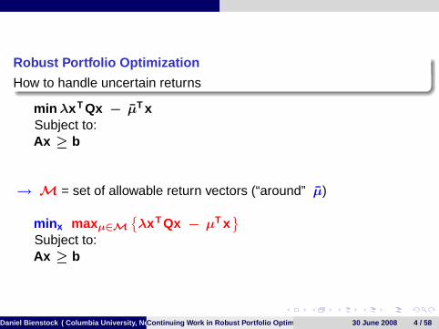
Robust Portfolio Optimization
How to handle uncertain returns
min λx T Qx − µT xSubject to:Ax ≥ b
→ M = set of allowable return vectors (“around” µ)
min x maxµ∈M{λx T Qx − µT x
}Subject to:Ax ≥ b
Daniel Bienstock ( Columbia University, New York)Continuing Work in Robust Portfolio Optimization 30 June 2008 4 / 58
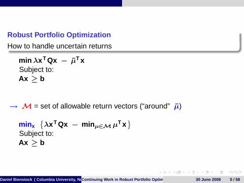
Robust Portfolio Optimization
How to handle uncertain returns
min λx T Qx − µT xSubject to:Ax ≥ b
→ M = set of allowable return vectors (“around” µ)
min x{λx T Qx − min µ∈M µT x
}Subject to:Ax ≥ b
Daniel Bienstock ( Columbia University, New York)Continuing Work in Robust Portfolio Optimization 30 June 2008 5 / 58
Robust Portfolio Optimization
How to handle uncertain returns
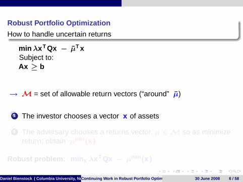
min λx T Qx − µT xSubject to:Ax ≥ b
→ M = set of allowable return vectors (“around” µ)
1 The investor chooses a vector x of assets
2 The adversary chooses a returns vector µ ∈M so as minimizereturn: obtain µmin (x )
Robust problem: min x λx T Qx − µmin (x )
Daniel Bienstock ( Columbia University, New York)Continuing Work in Robust Portfolio Optimization 30 June 2008 6 / 58
Robust Portfolio Optimization
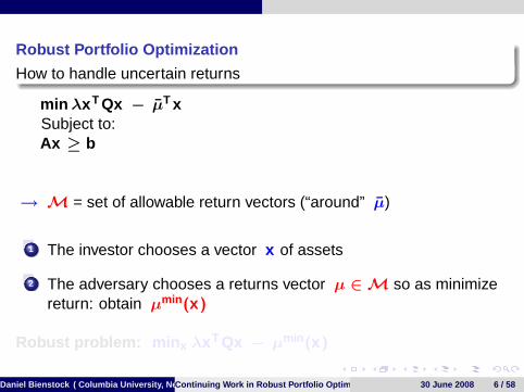
How to handle uncertain returns
min λx T Qx − µT xSubject to:Ax ≥ b
→ M = set of allowable return vectors (“around” µ)
1 The investor chooses a vector x of assets
2 The adversary chooses a returns vector µ ∈M so as minimizereturn: obtain µmin (x )
Robust problem: min x λx T Qx − µmin (x )
Daniel Bienstock ( Columbia University, New York)Continuing Work in Robust Portfolio Optimization 30 June 2008 6 / 58
Robust Portfolio Optimization
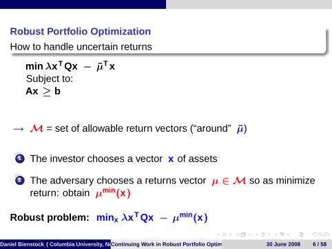
How to handle uncertain returns
min λx T Qx − µT xSubject to:Ax ≥ b
→ M = set of allowable return vectors (“around” µ)
1 The investor chooses a vector x of assets
2 The adversary chooses a returns vector µ ∈M so as minimizereturn: obtain µmin (x )
Robust problem: min x λx T Qx − µmin (x )
Daniel Bienstock ( Columbia University, New York)Continuing Work in Robust Portfolio Optimization 30 June 2008 6 / 58
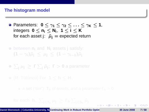
The histogram model
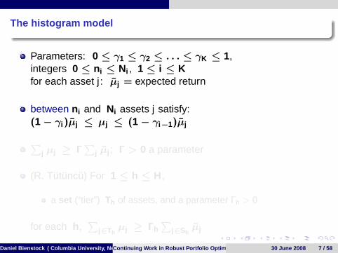
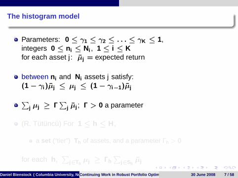
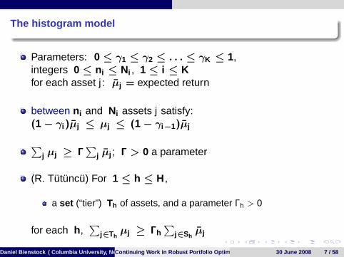
Parameters: 0 ≤ γ1 ≤ γ2 ≤ . . . ≤ γK ≤ 1,integers 0 ≤ n i ≤ Ni , 1 ≤ i ≤ Kfor each asset j : µj = expected return
between n i and Ni assets j satisfy:(1− γi )µj ≤ µj ≤ (1− γi−1)µj∑
j µj ≥ Γ∑
j µj ; Γ > 0 a parameter
(R. Tutuncu) For 1 ≤ h ≤ H,
a set (“tier”) Th of assets, and a parameter Γh > 0
for each h,∑
j∈Thµj ≥ Γh
∑j∈Sh
µj
Daniel Bienstock ( Columbia University, New York)Continuing Work in Robust Portfolio Optimization 30 June 2008 7 / 58
The histogram model
Parameters: 0 ≤ γ1 ≤ γ2 ≤ . . . ≤ γK ≤ 1,integers 0 ≤ n i ≤ Ni , 1 ≤ i ≤ Kfor each asset j : µj = expected return
between n i and Ni assets j satisfy:(1− γi )µj ≤ µj ≤ (1− γi−1)µj∑
j µj ≥ Γ∑
j µj ; Γ > 0 a parameter
(R. Tutuncu) For 1 ≤ h ≤ H,
a set (“tier”) Th of assets, and a parameter Γh > 0
for each h,∑
j∈Thµj ≥ Γh
∑j∈Sh
µj
Daniel Bienstock ( Columbia University, New York)Continuing Work in Robust Portfolio Optimization 30 June 2008 7 / 58
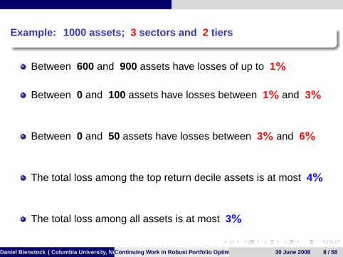
Example: 1000 assets; 3 sectors and 2 tiers
Between 600 and 900 assets have losses of up to 1%
Between 0 and 100 assets have losses between 1% and 3%
Between 0 and 50 assets have losses between 3% and 6%
The total loss among the top return decile assets is at most 4%
The total loss among all assets is at most 3%
Daniel Bienstock ( Columbia University, New York)Continuing Work in Robust Portfolio Optimization 30 June 2008 8 / 58
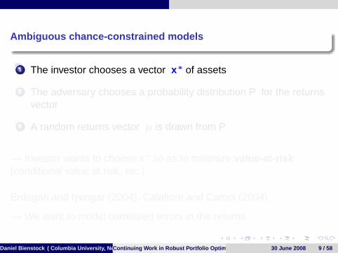
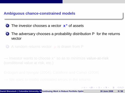
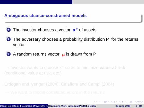
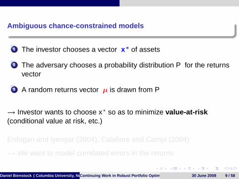
Ambiguous chance-constrained models
1 The investor chooses a vector x ∗ of assets
2 The adversary chooses a probability distribution P for the returnsvector
3 A random returns vector µ is drawn from P
→ Investor wants to choose x∗ so as to minimize value-at-risk(conditional value at risk, etc.)
Erdogan and Iyengar (2004), Calafiore and Campi (2004)
→We want to model correlated errors in the returns
Daniel Bienstock ( Columbia University, New York)Continuing Work in Robust Portfolio Optimization 30 June 2008 9 / 58
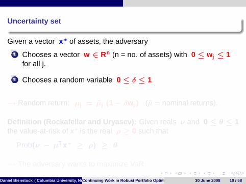
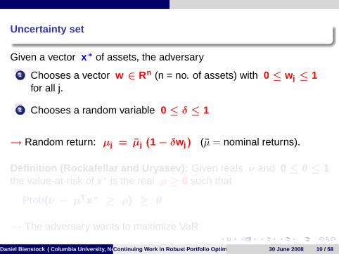
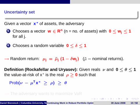
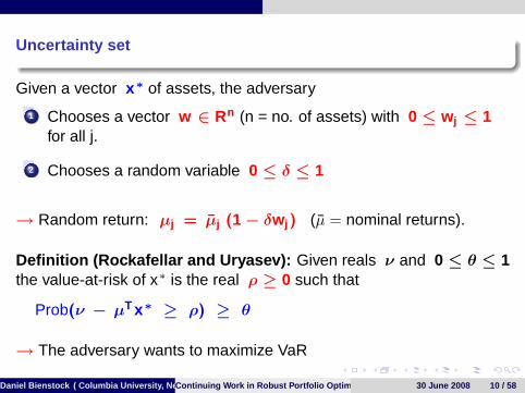
Uncertainty set
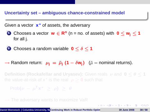
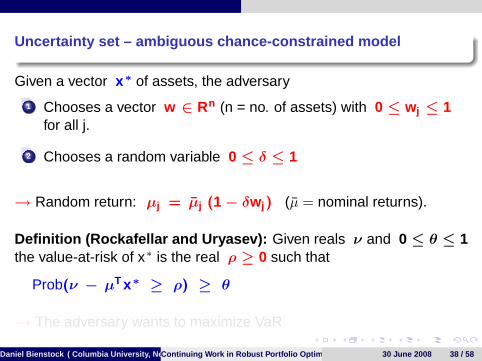
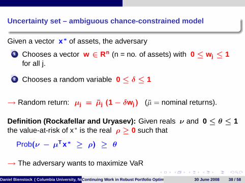
Given a vector x ∗ of assets, the adversary
1 Chooses a vector w ∈ Rn (n = no. of assets) with 0 ≤ w j ≤ 1for all j.
2 Chooses a random variable 0 ≤ δ ≤ 1
→ Random return: µj = µj (1− δw j ) (µ = nominal returns).
Definition (Rockafellar and Uryasev): Given reals ν and 0 ≤ θ ≤ 1the value-at-risk of x∗ is the real ρ ≥ 0 such that
Prob(ν − µT x ∗ ≥ ρ) ≥ θ
→ The adversary wants to maximize VaR
Daniel Bienstock ( Columbia University, New York)Continuing Work in Robust Portfolio Optimization 30 June 2008 10 / 58
Uncertainty set
Given a vector x ∗ of assets, the adversary
1 Chooses a vector w ∈ Rn (n = no. of assets) with 0 ≤ w j ≤ 1for all j.
2 Chooses a random variable 0 ≤ δ ≤ 1
→ Random return: µj = µj (1− δw j ) (µ = nominal returns).
Definition (Rockafellar and Uryasev): Given reals ν and 0 ≤ θ ≤ 1the value-at-risk of x∗ is the real ρ ≥ 0 such that
Prob(ν − µT x ∗ ≥ ρ) ≥ θ
→ The adversary wants to maximize VaR
Daniel Bienstock ( Columbia University, New York)Continuing Work in Robust Portfolio Optimization 30 June 2008 10 / 58
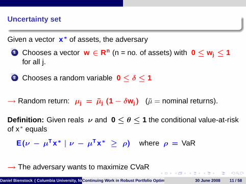
Uncertainty set
Given a vector x ∗ of assets, the adversary
1 Chooses a vector w ∈ Rn (n = no. of assets) with 0 ≤ w j ≤ 1for all j.
2 Chooses a random variable 0 ≤ δ ≤ 1
→ Random return: µj = µj (1− δw j ) (µ = nominal returns).
Definition: Given reals ν and 0 ≤ θ ≤ 1 the conditional value-at-riskof x∗ equals
E(ν − µT x ∗ | ν − µT x ∗ ≥ ρ) where ρ = VaR
→ The adversary wants to maximize CVaR
Daniel Bienstock ( Columbia University, New York)Continuing Work in Robust Portfolio Optimization 30 June 2008 11 / 58
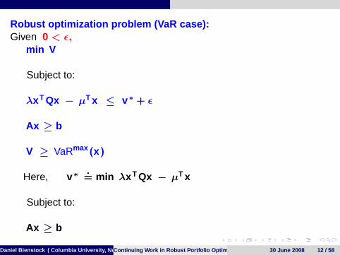
Robust optimization problem (VaR case):Given 0 < ε,
min V
Subject to:
λx T Qx − µT x ≤ v ∗ + ε
Ax ≥ b
V ≥ VaRmax (x )
Here, v ∗ .= min λx T Qx − µT x
Subject to:
Ax ≥ b
Daniel Bienstock ( Columbia University, New York)Continuing Work in Robust Portfolio Optimization 30 June 2008 12 / 58

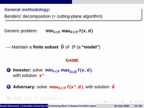
General methodology:
Benders’ decomposition (= cutting-plane algorithm)
Generic problem: min x∈X maxd∈D f (x , d )
→ Maintain a finite subset D of D (a “model” )
GAME
1 Investor: solve min x∈X maxd∈D f (x , d ),with solution x ∗
2 Adversary: solve maxd∈D f (x ∗, d ), with solution d
3 Add d to D, and go to 1.
Daniel Bienstock ( Columbia University, New York)Continuing Work in Robust Portfolio Optimization 30 June 2008 13 / 58
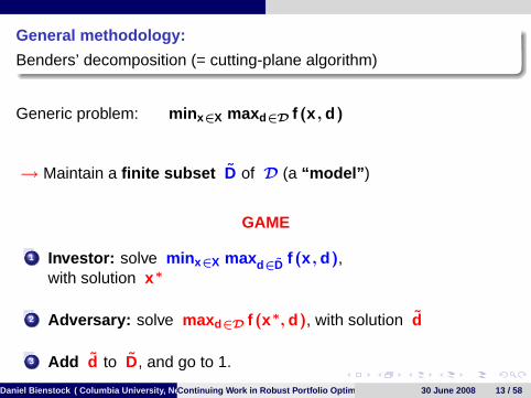

Why this approach
Decoupling of investor and adversary yields considerably simpler,and smaller, problems
Decoupling allows us to use more sophisticated uncertaintymodels
If number of iterations is small, investor’s problem is a small“convex” problem
Most progress will be achieved in initial iterations – permits “soft”termination criteria
Daniel Bienstock ( Columbia University, New York)Continuing Work in Robust Portfolio Optimization 30 June 2008 14 / 58
The game, applied to the robust optimization problem
Histogram version
Robust problem:
min x{λx T Qx − min µ∈M µT x
}Subject to:Ax ≥ b
Investor’s problem: M is replaced by a finite subset M
Daniel Bienstock ( Columbia University, New York)Continuing Work in Robust Portfolio Optimization 30 June 2008 15 / 58
Investor’s problem
A convex quadratic program
At iteration m, solve
min λx T Qx − r
Subject to:
Ax ≥ b
r ≤ µT(i )x , i = 1, . . . , m
Here, µ(1), . . . , µ(m) are given return vectors
Daniel Bienstock ( Columbia University, New York)Continuing Work in Robust Portfolio Optimization 30 June 2008 16 / 58
The game, applied to the robust optimization problem
Histogram version
Robust problem:
min x{λx T Qx − min µ∈M µT x
}Subject to:Ax ≥ b
Adversary’s problem: Given asset vector x , solve min µ∈M µT x
Daniel Bienstock ( Columbia University, New York)Continuing Work in Robust Portfolio Optimization 30 June 2008 17 / 58
Back to the histogram model
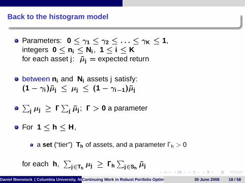
Parameters: 0 ≤ γ1 ≤ γ2 ≤ . . . ≤ γK ≤ 1,integers 0 ≤ n i ≤ Ni , 1 ≤ i ≤ Kfor each asset j : µj = expected return
between n i and Ni assets j satisfy:(1− γi )µj ≤ µj ≤ (1− γi−1)µj∑
j µj ≥ Γ∑
j µj ; Γ > 0 a parameter
For 1 ≤ h ≤ H,
a set (“tier”) Th of assets, and a parameter Γh > 0
for each h,∑
j∈Thµj ≥ Γh
∑j∈Sh
µj
Daniel Bienstock ( Columbia University, New York)Continuing Work in Robust Portfolio Optimization 30 June 2008 18 / 58
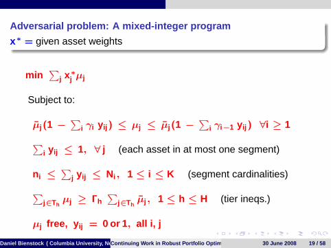
Adversarial problem: A mixed-integer program
x ∗ = given asset weights
min∑
j x ∗j µj
Subject to:
µj (1 −∑
i γi y ij ) ≤ µj ≤ µj (1 −∑
i γi−1 y ij ) ∀i ≥ 1∑i y ij ≤ 1, ∀ j (each asset in at most one segment)
n i ≤∑
j y ij ≤ Ni , 1 ≤ i ≤ K (segment cardinalities)∑j∈Th
µj ≥ Γh∑
j∈Thµj , 1 ≤ h ≤ H (tier ineqs.)
µj free, y ij = 0 or 1 , all i, j
Daniel Bienstock ( Columbia University, New York)Continuing Work in Robust Portfolio Optimization 30 June 2008 19 / 58
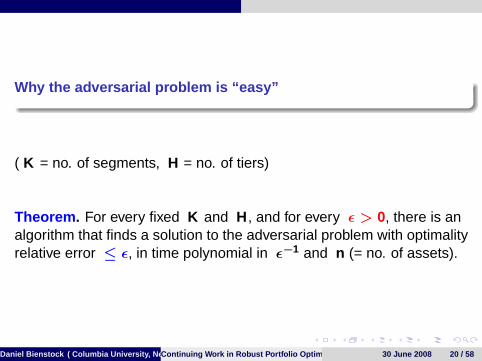
Why the adversarial problem is “easy”
( K = no. of segments, H = no. of tiers)
Theorem . For every fixed K and H, and for every ε > 0, there is analgorithm that finds a solution to the adversarial problem with optimalityrelative error ≤ ε, in time polynomial in ε−1 and n (= no. of assets).
Daniel Bienstock ( Columbia University, New York)Continuing Work in Robust Portfolio Optimization 30 June 2008 20 / 58
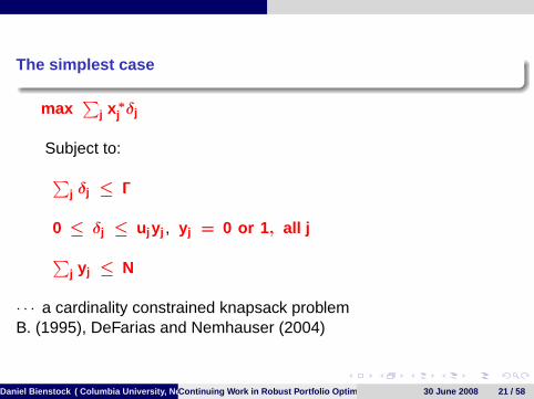
The simplest case
max∑
j x ∗j δj
Subject to:∑j δj ≤ Γ
0 ≤ δj ≤ u j y j , y j = 0 or 1 , all j∑j y j ≤ N
· · · a cardinality constrained knapsack problemB. (1995), DeFarias and Nemhauser (2004)
Daniel Bienstock ( Columbia University, New York)Continuing Work in Robust Portfolio Optimization 30 June 2008 21 / 58

Summary
At each iteration of the game, we solve:
1 A convex quadratic program – a new constraint added everyiteration
2 A mixed-integer program, always of the same size.
Questions:
How fast (slow?) is each iteration?
How many iterations?
Daniel Bienstock ( Columbia University, New York)Continuing Work in Robust Portfolio Optimization 30 June 2008 22 / 58
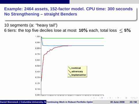
Example: 2464 assets, 152-factor model. CPU time: 300 secondsNo Strengthening – straight Benders
10 segments (a: “heavy tail”)6 tiers: the top five deciles lose at most 10% each, total loss ≤ 5%
Daniel Bienstock ( Columbia University, New York)Continuing Work in Robust Portfolio Optimization 30 June 2008 23 / 58
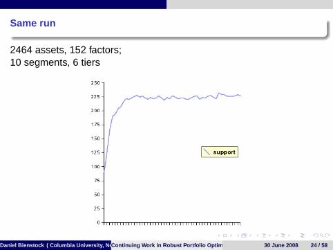
Same run
2464 assets, 152 factors;10 segments, 6 tiers
Daniel Bienstock ( Columbia University, New York)Continuing Work in Robust Portfolio Optimization 30 June 2008 24 / 58
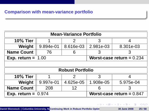
Comparison with mean-variance portfolio
Mean-Variance Portfolio10% Tier 1 2 3 4
Weight 9.894e-01 8.616e-03 2.981e-03 8.301e-03Name Count 76 6 3 3Exp. return = 1.00 Worst-case return = 0.234
Robust Portfolio10% Tier 1 2 3 4
Weight 9.997e-01 4.625e-05 1.908e-05 5.975e-04Name Count 208 12 6 3Exp. return = 0.974 Worst-case return = 0.847
Daniel Bienstock ( Columbia University, New York)Continuing Work in Robust Portfolio Optimization 30 June 2008 25 / 58
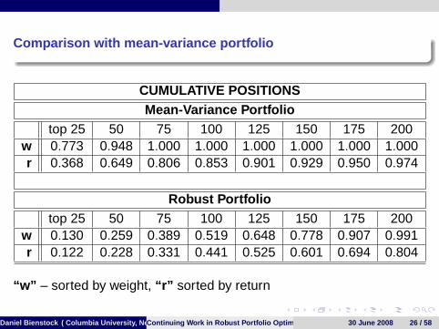
Comparison with mean-variance portfolio
CUMULATIVE POSITIONSMean-Variance Portfolio
top 25 50 75 100 125 150 175 200w 0.773 0.948 1.000 1.000 1.000 1.000 1.000 1.000r 0.368 0.649 0.806 0.853 0.901 0.929 0.950 0.974
Robust Portfoliotop 25 50 75 100 125 150 175 200
w 0.130 0.259 0.389 0.519 0.648 0.778 0.907 0.991r 0.122 0.228 0.331 0.441 0.525 0.601 0.694 0.804
“w” – sorted by weight, “r” sorted by return
Daniel Bienstock ( Columbia University, New York)Continuing Work in Robust Portfolio Optimization 30 June 2008 26 / 58
Comparison with mean-variance portfolio
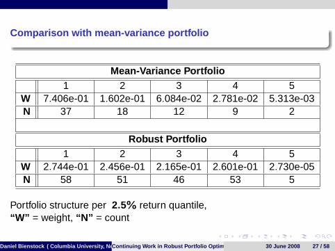
Mean-Variance Portfolio1 2 3 4 5
W 7.406e-01 1.602e-01 6.084e-02 2.781e-02 5.313e-03N 37 18 12 9 2
Robust Portfolio1 2 3 4 5
W 2.744e-01 2.456e-01 2.165e-01 2.601e-01 2.730e-05N 58 51 46 53 5
Portfolio structure per 2.5% return quantile,“W” = weight, “N” = count
Daniel Bienstock ( Columbia University, New York)Continuing Work in Robust Portfolio Optimization 30 June 2008 27 / 58

A popular heuristic
→ Impose the constraint x j ≤ w for all assets j
Here, w is a “small” value
Nomenclature: heuristic portfolio U-w
Daniel Bienstock ( Columbia University, New York)Continuing Work in Robust Portfolio Optimization 30 June 2008 28 / 58

A popular heuristic
→ Impose the constraint x j ≤ w for all assets j
Here, w is a “small” value
Nomenclature: heuristic portfolio U-w
Daniel Bienstock ( Columbia University, New York)Continuing Work in Robust Portfolio Optimization 30 June 2008 28 / 58
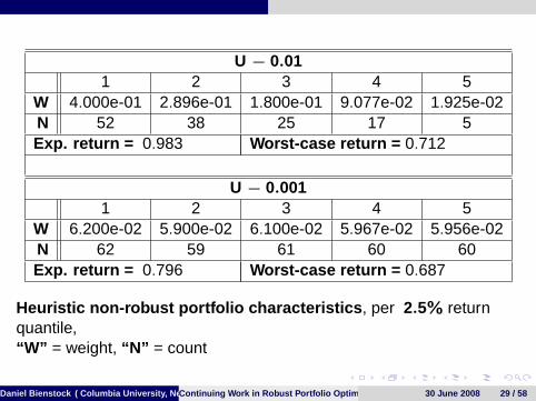
U − 0.011 2 3 4 5
W 4.000e-01 2.896e-01 1.800e-01 9.077e-02 1.925e-02N 52 38 25 17 5Exp. return = 0.983 Worst-case return = 0.712
U − 0.0011 2 3 4 5
W 6.200e-02 5.900e-02 6.100e-02 5.967e-02 5.956e-02N 62 59 61 60 60Exp. return = 0.796 Worst-case return = 0.687
Heuristic non-robust portfolio characteristics , per 2.5% returnquantile,“W” = weight, “N” = count
Daniel Bienstock ( Columbia University, New York)Continuing Work in Robust Portfolio Optimization 30 June 2008 29 / 58
Updated heuristic
→ Impose the constraint x j ≤ w for all assets j in return decile 1
Nomenclature: heuristic portfolio T-w
Daniel Bienstock ( Columbia University, New York)Continuing Work in Robust Portfolio Optimization 30 June 2008 30 / 58
Updated heuristic
→ Impose the constraint x j ≤ w for all assets j in return decile 1
Nomenclature: heuristic portfolio T-w
Daniel Bienstock ( Columbia University, New York)Continuing Work in Robust Portfolio Optimization 30 June 2008 30 / 58
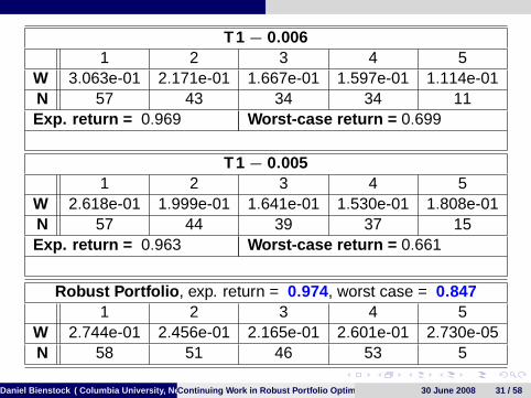
T 1− 0.0061 2 3 4 5
W 3.063e-01 2.171e-01 1.667e-01 1.597e-01 1.114e-01N 57 43 34 34 11Exp. return = 0.969 Worst-case return = 0.699
T 1− 0.0051 2 3 4 5
W 2.618e-01 1.999e-01 1.641e-01 1.530e-01 1.808e-01N 57 44 39 37 15Exp. return = 0.963 Worst-case return = 0.661
Robust Portfolio , exp. return = 0.974, worst case = 0.8471 2 3 4 5
W 2.744e-01 2.456e-01 2.165e-01 2.601e-01 2.730e-05N 58 51 46 53 5
Daniel Bienstock ( Columbia University, New York)Continuing Work in Robust Portfolio Optimization 30 June 2008 31 / 58
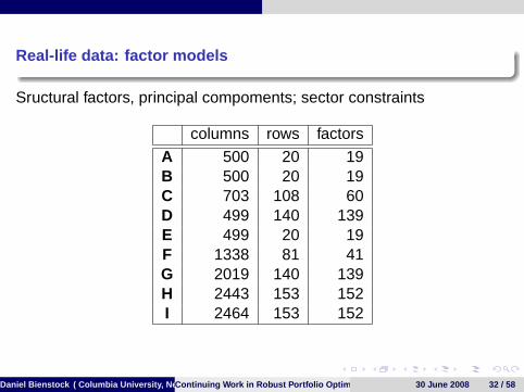
Real-life data: factor models
Sructural factors, principal compoments; sector constraints
columns rows factors
A 500 20 19B 500 20 19C 703 108 60D 499 140 139E 499 20 19F 1338 81 41G 2019 140 139H 2443 153 152I 2464 153 152
Daniel Bienstock ( Columbia University, New York)Continuing Work in Robust Portfolio Optimization 30 June 2008 32 / 58
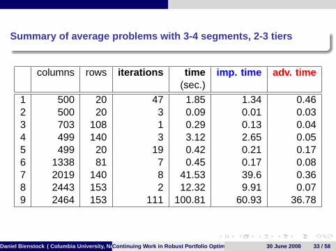
Summary of average problems with 3-4 segments, 2-3 tiers
columns rows iterations time imp. time adv. time(sec.)
1 500 20 47 1.85 1.34 0.462 500 20 3 0.09 0.01 0.033 703 108 1 0.29 0.13 0.044 499 140 3 3.12 2.65 0.055 499 20 19 0.42 0.21 0.176 1338 81 7 0.45 0.17 0.087 2019 140 8 41.53 39.6 0.368 2443 153 2 12.32 9.91 0.079 2464 153 111 100.81 60.93 36.78
Daniel Bienstock ( Columbia University, New York)Continuing Work in Robust Portfolio Optimization 30 June 2008 33 / 58
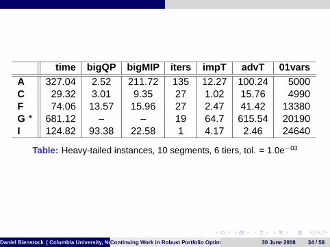
time bigQP bigMIP iters impT advT 01varsA 327.04 2.52 211.72 135 12.27 100.24 5000C 29.32 3.01 9.35 27 1.02 15.76 4990F 74.06 13.57 15.96 27 2.47 41.42 13380G ∗ 681.12 – – 19 64.7 615.54 20190I 124.82 93.38 22.58 1 4.17 2.46 24640
Table: Heavy-tailed instances, 10 segments, 6 tiers, tol. = 1.0e−03
Daniel Bienstock ( Columbia University, New York)Continuing Work in Robust Portfolio Optimization 30 June 2008 34 / 58
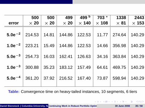
500 500 499 499 b 703 ∗ 1338 2443error × 20 × 20 × 20 × 140 × 108 × 81 × 153
5.0e−2 214.53 14.81 144.86 122.53 11.77 274.64 140.29
1.0e−2 223.21 15.49 144.86 122.53 14.66 356.98 140.29
5.0e−3 254.73 16.03 162.41 126.63 34.16 363.84 140.29
1.0e−3 300.88 35.23 183.12 157.49 64.61 469.75 140.29
5.0e−4 361.20 37.92 216.52 167.40 73.87 598.94 140.29
Table: Convergence time on heavy-tailed instances, 10 segments, 6 tiers
Daniel Bienstock ( Columbia University, New York)Continuing Work in Robust Portfolio Optimization 30 June 2008 35 / 58
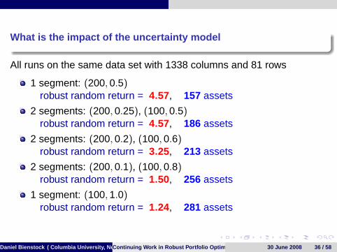
What is the impact of the uncertainty model
All runs on the same data set with 1338 columns and 81 rows
1 segment: (200, 0.5)robust random return = 4.57, 157 assets
2 segments: (200, 0.25), (100, 0.5)robust random return = 4.57, 186 assets
2 segments: (200, 0.2), (100, 0.6)robust random return = 3.25, 213 assets
2 segments: (200, 0.1), (100, 0.8)robust random return = 1.50, 256 assets
1 segment: (100, 1.0)robust random return = 1.24, 281 assets
Daniel Bienstock ( Columbia University, New York)Continuing Work in Robust Portfolio Optimization 30 June 2008 36 / 58
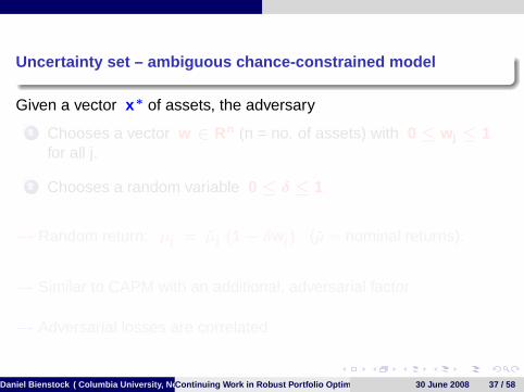
Uncertainty set – ambiguous chance-constrained model
Given a vector x ∗ of assets, the adversary
1 Chooses a vector w ∈ Rn (n = no. of assets) with 0 ≤ w j ≤ 1for all j.
2 Chooses a random variable 0 ≤ δ ≤ 1
→ Random return: µj = µj (1− δw j ) (µ = nominal returns).
→ Similar to CAPM with an additional, adversarial factor
→ Adversarial losses are correlated
Daniel Bienstock ( Columbia University, New York)Continuing Work in Robust Portfolio Optimization 30 June 2008 37 / 58
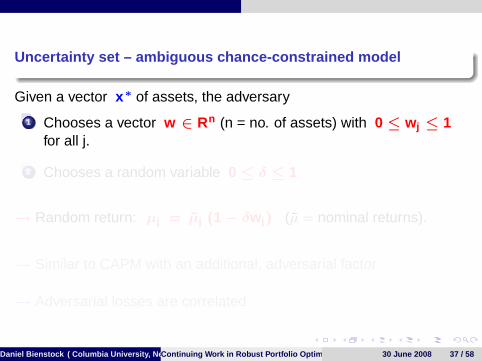
Uncertainty set – ambiguous chance-constrained model
Given a vector x ∗ of assets, the adversary
1 Chooses a vector w ∈ Rn (n = no. of assets) with 0 ≤ w j ≤ 1for all j.
2 Chooses a random variable 0 ≤ δ ≤ 1
→ Random return: µj = µj (1− δw j ) (µ = nominal returns).
Definition (Rockafellar and Uryasev): Given reals ν and 0 ≤ θ ≤ 1the value-at-risk of x∗ is the real ρ ≥ 0 such that
Prob(ν − µT x ∗ ≥ ρ) ≥ θ
→ The adversary wants to maximize VaR
Daniel Bienstock ( Columbia University, New York)Continuing Work in Robust Portfolio Optimization 30 June 2008 38 / 58
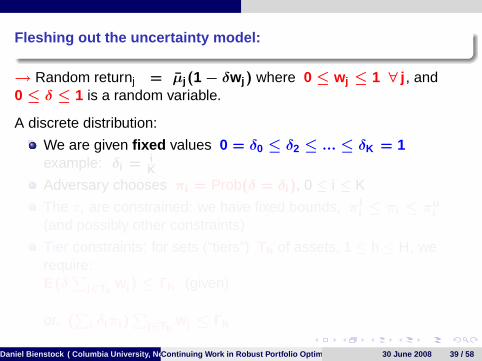
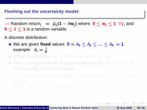
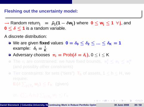
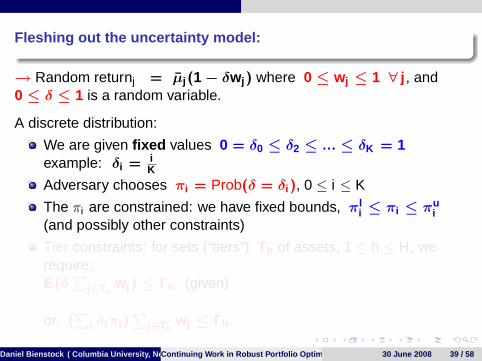
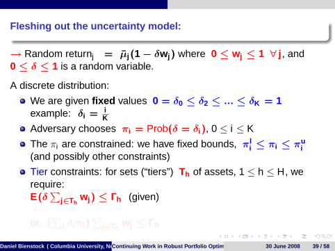
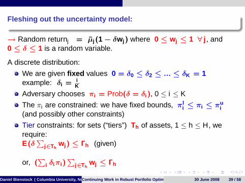
Fleshing out the uncertainty model:
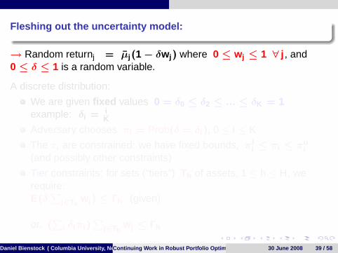
→ Random returnj = µj (1− δw j ) where 0 ≤ w j ≤ 1 ∀ j , and0 ≤ δ ≤ 1 is a random variable.
A discrete distribution:
We are given fixed values 0 = δ0 ≤ δ2 ≤ ... ≤ δK = 1example: δi = i
K
Adversary chooses πi = Prob(δ = δi ), 0 ≤ i ≤ K
The πi are constrained: we have fixed bounds, πli ≤ πi ≤ πu
i(and possibly other constraints)
Tier constraints: for sets (“tiers”) Th of assets, 1 ≤ h ≤ H, werequire:E(δ
∑j∈Th
w j ) ≤ Γh (given)
or, (∑
i δi πi )∑
j∈Thw j ≤ Γh
Daniel Bienstock ( Columbia University, New York)Continuing Work in Robust Portfolio Optimization 30 June 2008 39 / 58
Fleshing out the uncertainty model:
→ Random returnj = µj (1− δw j ) where 0 ≤ w j ≤ 1 ∀ j , and0 ≤ δ ≤ 1 is a random variable.
A discrete distribution:
We are given fixed values 0 = δ0 ≤ δ2 ≤ ... ≤ δK = 1example: δi = i
K
Adversary chooses πi = Prob(δ = δi ), 0 ≤ i ≤ K
The πi are constrained: we have fixed bounds, πli ≤ πi ≤ πu
i(and possibly other constraints)
Tier constraints: for sets (“tiers”) Th of assets, 1 ≤ h ≤ H, werequire:E(δ
∑j∈Th
w j ) ≤ Γh (given)
or, (∑
i δi πi )∑
j∈Thw j ≤ Γh
Daniel Bienstock ( Columbia University, New York)Continuing Work in Robust Portfolio Optimization 30 June 2008 39 / 58

Robust optimization problem (VaR case):Given 0 < ε,
min V
Subject to:
λx T Qx − µT x ≤ v ∗ + ε
Ax ≥ b
V ≥ VaRmax (x )
Here, v ∗ .= min λx T Qx − µT x
Subject to:
Ax ≥ b
Daniel Bienstock ( Columbia University, New York)Continuing Work in Robust Portfolio Optimization 30 June 2008 40 / 58
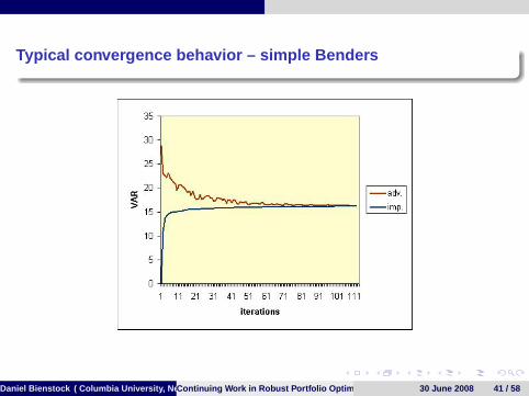
Typical convergence behavior – simple Benders
Daniel Bienstock ( Columbia University, New York)Continuing Work in Robust Portfolio Optimization 30 June 2008 41 / 58
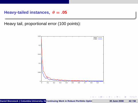
Heavy-tailed instances, θ = .05
Heavy tail, proportional error (100 points):
0
0.05
0.1
0.15
0.2
0.25
0 0.1 0.2 0.3 0.4 0.5 0.6 0.7 0.8 0.9 1
UpperLower
Daniel Bienstock ( Columbia University, New York)Continuing Work in Robust Portfolio Optimization 30 June 2008 42 / 58
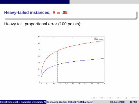
Heavy-tailed instances, θ = .05
Heavy tail, proportional error (100 points):
0
0.2
0.4
0.6
0.8
1
1.2
1.4
0 0.1 0.2 0.3 0.4 0.5 0.6 0.7 0.8 0.9 1
UpperLower
Daniel Bienstock ( Columbia University, New York)Continuing Work in Robust Portfolio Optimization 30 June 2008 42 / 58
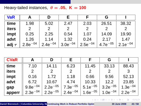
Heavy-tailed instances, θ = .05, K = 100
VaR A D E F G Itime 1.98 5.02 2.47 2.03 26.51 38.32iters 2 2 2 2 2 2impt 0.25 2.25 0.54 1.07 14.09 19.90advt 1.26 1.14 1.32 0.24 2.17 1.47adj τ 2.8e−04 2.4e−04 3.0e−04 2.5e−04 4.7e−05 2.1e−04
CVaR A D E F G Itime 7.10 14.11 6.23 11.45 33.13 88.43iters 2 2 2 2 2 3impt 0.16 1.72 1.18 0.66 9.56 52.13advt 6.72 10.67 4.74 10.33 12.2 23.85gap 9.8e−04 2.2e−05 7.3e−05 5.1e−05 3.2e−05 1.3e−04
apperr 2.3e−04 2.2e−05 2.4e−04 1.6e−05 1.0e−04 2.2e−04
Daniel Bienstock ( Columbia University, New York)Continuing Work in Robust Portfolio Optimization 30 June 2008 43 / 58
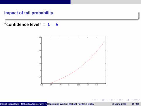
Impact of tail probability
“confidence level” = 1− θ
1
1.5
2
2.5
3
3.5
4
4.5
0.65 0.7 0.75 0.8 0.85 0.9 0.95 1
Daniel Bienstock ( Columbia University, New York)Continuing Work in Robust Portfolio Optimization 30 June 2008 44 / 58
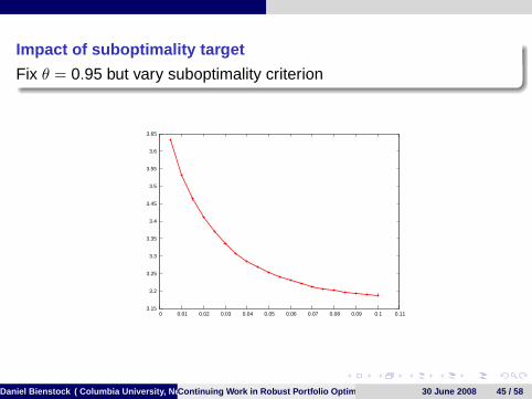
Impact of suboptimality target
Fix θ = 0.95 but vary suboptimality criterion
3.15
3.2
3.25
3.3
3.35
3.4
3.45
3.5
3.55
3.6
3.65
0 0.01 0.02 0.03 0.04 0.05 0.06 0.07 0.08 0.09 0.1 0.11
Daniel Bienstock ( Columbia University, New York)Continuing Work in Robust Portfolio Optimization 30 June 2008 45 / 58
Experiment: sensitivity of model to parameters
Adversary chooses πi = P(δ = δi ), πli ≤ πi ≤ πu
i
Experiment: choose ∆ ≥ 0, and solve robust problems for
πli ← max{πl
i −∆, 0}, πui ← πu
i + ∆
Daniel Bienstock ( Columbia University, New York)Continuing Work in Robust Portfolio Optimization 30 June 2008 46 / 58
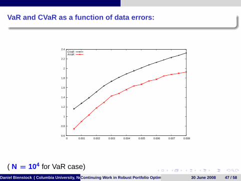
VaR and CVaR as a function of data errors:
0.6
0.8
1
1.2
1.4
1.6
1.8
2
2.2
2.4
0 0.001 0.002 0.003 0.004 0.005 0.006 0.007 0.008
CVaRAVaR
( N = 104 for VaR case)Daniel Bienstock ( Columbia University, New York)Continuing Work in Robust Portfolio Optimization 30 June 2008 47 / 58

Part II: Methodology
Daniel Bienstock ( Columbia University, New York)Continuing Work in Robust Portfolio Optimization 30 June 2008 48 / 58
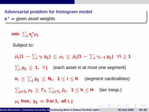
Adversarial problem for histogram model
x ∗ = given asset weights
min∑
j x ∗j µj
Subject to:
µj (1 −∑
i γi y ij ) ≤ µj ≤ µj (1 −∑
i γi−1 y ij ) ∀i ≥ 1∑i y ij ≤ 1, ∀ j (each asset in at most one segment)
n i ≤∑
j y ij ≤ Ni , 1 ≤ i ≤ K (segment cardinalities)∑j∈Th
µj ≥ Γh∑
j∈Thµj , 1 ≤ h ≤ H (tier ineqs.)
µj free, y ij = 0 or 1 , all i, j
Daniel Bienstock ( Columbia University, New York)Continuing Work in Robust Portfolio Optimization 30 June 2008 49 / 58
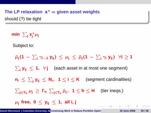
The LP relaxation x ∗ = given asset weights
should (?) be tight
min∑
j x ∗j µj
Subject to:
µj (1 −∑
i γi−1 y ij ) ≤ µj ≤ µj (1 −∑
i γi y ij ) ∀i ≥ 1∑i y ij ≤ 1, ∀ j (each asset in at most one segment)
n i ≤∑
j y ij ≤ Ni , 1 ≤ i ≤ K (segment cardinalities)∑j∈Th
µj ≥ Γh∑
j∈Thµj , 1 ≤ h ≤ H (tier ineqs.)
µj free, 0 ≤ y ij ≤ 1, all i, j
Daniel Bienstock ( Columbia University, New York)Continuing Work in Robust Portfolio Optimization 30 June 2008 50 / 58
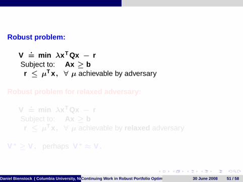
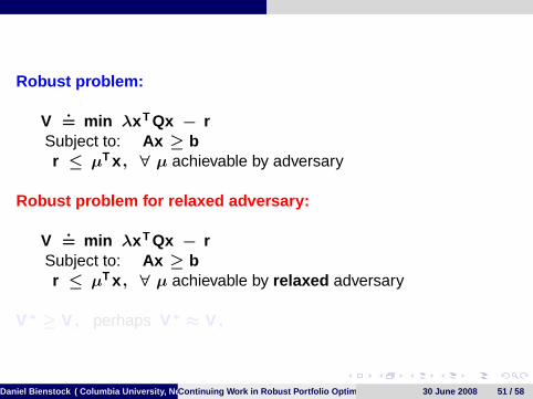
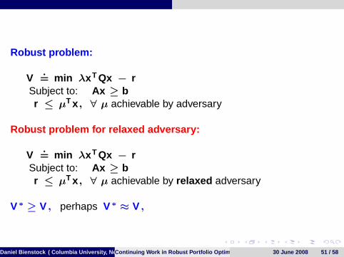
Robust problem:
V.= min λx T Qx − r
Subject to: Ax ≥ br ≤ µT x , ∀ µ achievable by adversary
Robust problem for relaxed adversary:
V.= min λx T Qx − r
Subject to: Ax ≥ br ≤ µT x , ∀ µ achievable by relaxed adversary
V ∗ ≥ V , perhaps V ∗ ≈ V ,
Daniel Bienstock ( Columbia University, New York)Continuing Work in Robust Portfolio Optimization 30 June 2008 51 / 58
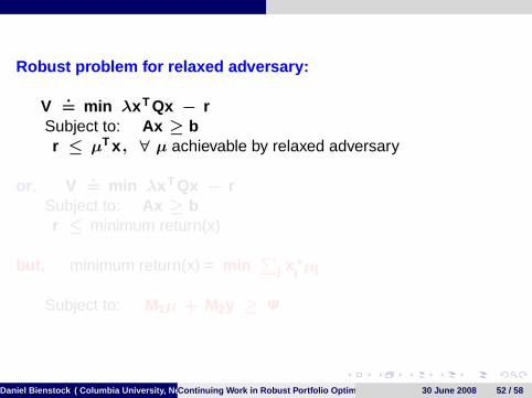
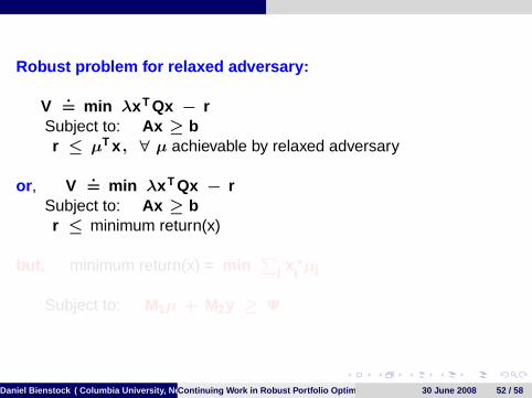
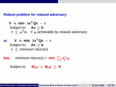
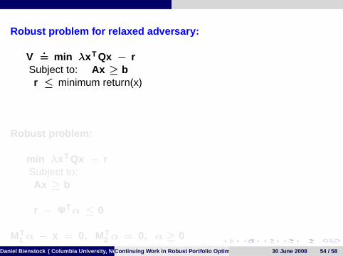
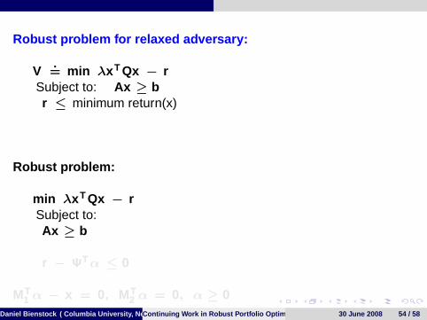
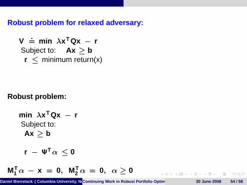
Robust problem for relaxed adversary:
V.= min λx T Qx − r
Subject to: Ax ≥ br ≤ µT x , ∀ µ achievable by relaxed adversary
or , V.= min λx T Qx − r
Subject to: Ax ≥ br ≤ minimum return(x)
but, minimum return(x) = min∑
j x ∗j µj
Subject to: M1µ + M2y ≥ Ψ
Daniel Bienstock ( Columbia University, New York)Continuing Work in Robust Portfolio Optimization 30 June 2008 52 / 58
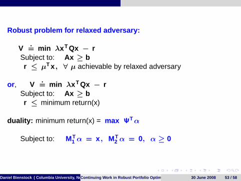
Robust problem for relaxed adversary:
V.= min λx T Qx − r
Subject to: Ax ≥ br ≤ µT x , ∀ µ achievable by relaxed adversary
or , V.= min λx T Qx − r
Subject to: Ax ≥ br ≤ minimum return(x)
duality: minimum return(x) = max ΨT α
Subject to: MT1 α = x , MT
2 α = 0, α ≥ 0
Daniel Bienstock ( Columbia University, New York)Continuing Work in Robust Portfolio Optimization 30 June 2008 53 / 58
Robust problem for relaxed adversary:
V.= min λx T Qx − r
Subject to: Ax ≥ br ≤ minimum return(x)
Robust problem:
min λx T Qx − rSubject to:Ax ≥ b
r − ΨT α ≤ 0
MT1 α − x = 0, MT
2 α = 0, α ≥ 0Daniel Bienstock ( Columbia University, New York)Continuing Work in Robust Portfolio Optimization 30 June 2008 54 / 58
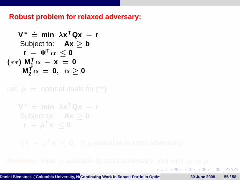
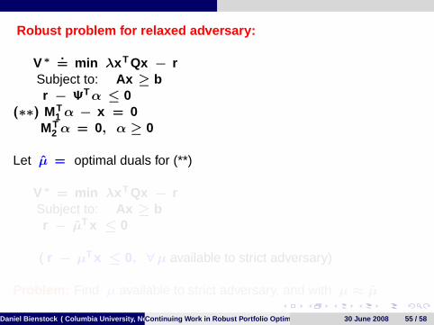
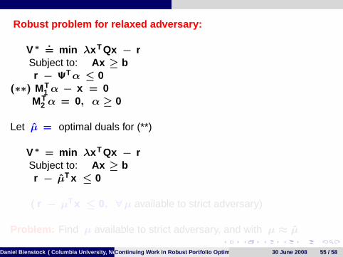
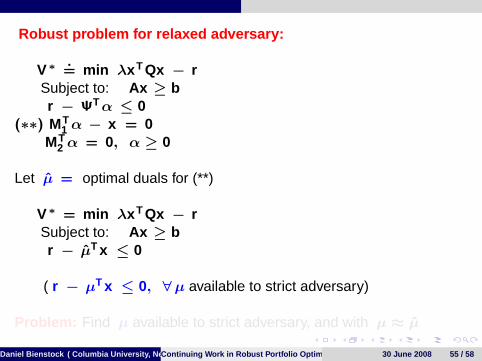
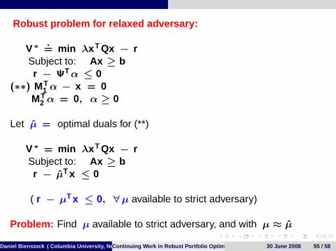
Robust problem for relaxed adversary:
V ∗ .= min λx T Qx − r
Subject to: Ax ≥ br − ΨT α ≤ 0
(∗∗) MT1 α − x = 0
MT2 α = 0, α ≥ 0
Let µ = optimal duals for (**)
V ∗ = min λx T Qx − rSubject to: Ax ≥ br − µT x ≤ 0
( r − µT x ≤ 0, ∀µ available to strict adversary)
Problem: Find µ available to strict adversary, and with µ ≈ µ
Daniel Bienstock ( Columbia University, New York)Continuing Work in Robust Portfolio Optimization 30 June 2008 55 / 58
Benders’ algorithm with strengthening
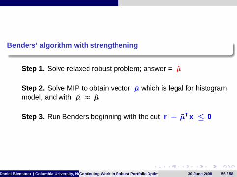
Step 1. Solve relaxed robust problem; answer = µ
Step 2. Solve MIP to obtain vector µ which is legal for histogrammodel, and with µ ≈ µ
Step 3. Run Benders beginning with the cut r − µT x ≤ 0
Daniel Bienstock ( Columbia University, New York)Continuing Work in Robust Portfolio Optimization 30 June 2008 56 / 58
Alternate algorithm?
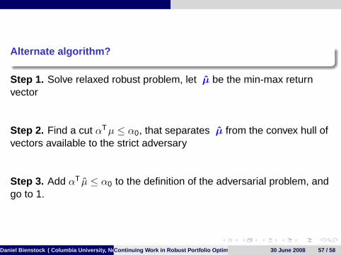
Step 1. Solve relaxed robust problem, let µ be the min-max returnvector
Step 2. Find a cut αT µ ≤ α0, that separates µ from the convex hull ofvectors available to the strict adversary
Step 3. Add αT µ ≤ α0 to the definition of the adversarial problem, andgo to 1.
Daniel Bienstock ( Columbia University, New York)Continuing Work in Robust Portfolio Optimization 30 June 2008 57 / 58
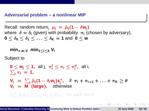
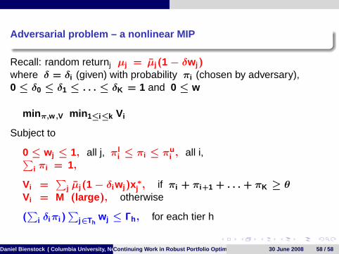
Adversarial problem – a nonlinear MIP
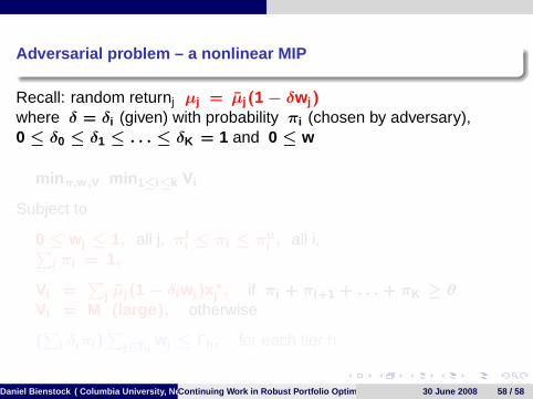
Recall: random returnj µj = µj (1− δw j )where δ = δi (given) with probability πi (chosen by adversary),0 ≤ δ0 ≤ δ1 ≤ . . . ≤ δK = 1 and 0 ≤ w
min π,w ,V min 1≤i≤k Vi
Subject to
0 ≤ w j ≤ 1, all j, πli ≤ πi ≤ πu
i , all i,∑i πi = 1,
Vi =∑
j µj (1− δi w j )x ∗j , if πi + πi+1 + . . . + πK ≥ θ
Vi = M (large ), otherwise
(∑
i δi πi )∑
j∈Thw j ≤ Γh , for each tier h
Daniel Bienstock ( Columbia University, New York)Continuing Work in Robust Portfolio Optimization 30 June 2008 58 / 58
Adversarial problem – a nonlinear MIP
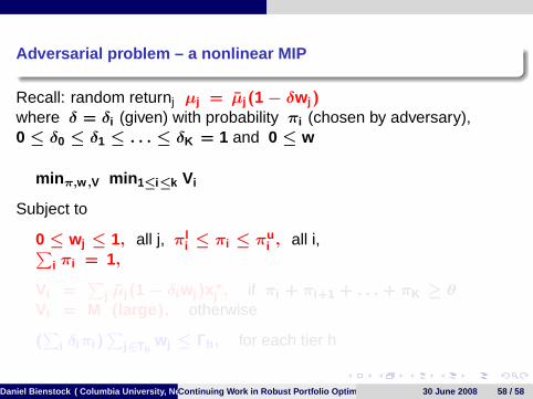
Recall: random returnj µj = µj (1− δw j )where δ = δi (given) with probability πi (chosen by adversary),0 ≤ δ0 ≤ δ1 ≤ . . . ≤ δK = 1 and 0 ≤ w
min π,w ,V min 1≤i≤k Vi
Subject to
0 ≤ w j ≤ 1, all j, πli ≤ πi ≤ πu
i , all i,∑i πi = 1,
Vi =∑
j µj (1− δi w j )x ∗j , if πi + πi+1 + . . . + πK ≥ θ
Vi = M (large ), otherwise
(∑
i δi πi )∑
j∈Thw j ≤ Γh , for each tier h
Daniel Bienstock ( Columbia University, New York)Continuing Work in Robust Portfolio Optimization 30 June 2008 58 / 58
Adversarial problem – a nonlinear MIP
Recall: random returnj µj = µj (1− δw j )where δ = δi (given) with probability πi (chosen by adversary),0 ≤ δ0 ≤ δ1 ≤ . . . ≤ δK = 1 and 0 ≤ w
min π,w ,V min 1≤i≤k Vi
Subject to
0 ≤ w j ≤ 1, all j, πli ≤ πi ≤ πu
i , all i,∑i πi = 1,
Vi =∑
j µj (1− δi w j )x ∗j , if πi + πi+1 + . . . + πK ≥ θ
Vi = M (large ), otherwise
(∑
i δi πi )∑
j∈Thw j ≤ Γh , for each tier h
Daniel Bienstock ( Columbia University, New York)Continuing Work in Robust Portfolio Optimization 30 June 2008 58 / 58

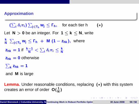
Approximation
(∑
i δi πi )∑
j∈Thw j ≤ Γh , for each tier h (∗)
Let N > 0 be an integer. For 1 ≤ k ≤ N , write
kN
∑j∈Th
w j ≤ Γh + M (1− zhk ), where
zhk = 1 if k −1N <
∑i δi πi ≤ k
N
zhk = 0 otherwise∑k zhk = 1
and M is large
Lemma. Under reasonable conditions, replacing (∗) with this systemcreates an error of order O( 1
N )
Daniel Bienstock ( Columbia University, New York)Continuing Work in Robust Portfolio Optimization 30 June 2008 59 / 58