Context Matters: A Theory of Semantic Discriminability for ...
16
Context Matters: A Theory of Semantic Discriminability for Perceptual Encoding Systems Kushin Mukherjee, Brian Yin, Brianne E. Sherman, Laurent Lessard, and Karen B. Schloss 1 0 ΔS Frequency Frequency Frequency Large distribution difference Medium distribution difference Small distribution difference High capacity for semantic discriminability Medium capacity for semantic discriminability Low capacity for semantic discriminability 1 0 1 0 peach celery driving comfort eggplant grape Association Association max ΔS max ΔS max ΔS Figure 1: Color-concept association distributions for concept pairs with large, medium, and small distribution differences, resulting in high, medium, and low capacities for semantic discriminability, respectively (terms defined in Section 3). Color-concept association ratings were collected in Experiment 1 for the UW-71 colors (colored stripes in the plots, sorted by CIE LCh hue angle). Abstract— People’s associations between colors and concepts influence their ability to interpret the meanings of colors in information visualizations. Previous work has suggested such effects are limited to concepts that have strong, specific associations with colors. However, although a concept may not be strongly associated with any colors, its mapping can be disambiguated in the context of other concepts in an encoding system. We articulate this view in semantic discriminability theory, a general framework for understanding conditions determining when people can infer meaning from perceptual features. Semantic discriminability is the degree to which observers can infer a unique mapping between visual features and concepts. Semantic discriminability theory posits that the capacity for semantic discriminability for a set of concepts is constrained by the difference between the feature-concept association distributions across the concepts in the set. We define formal properties of this theory and test its implications in two experiments. The results show that the capacity to produce semantically discriminable colors for sets of concepts was indeed constrained by the statistical distance between color-concept association distributions (Experiment 1). Moreover, people could interpret meanings of colors in bar graphs insofar as the colors were semantically discriminable, even for concepts previously considered “non-colorable” (Experiment 2). The results suggest that colors are more robust for visual communication than previously thought. Index Terms—Visual Reasoning, Information Visualization, Visual Communication, Visual Encoding, Color Cognition 1 I NTRODUCTION Bananas are shades of yellow, blueberries are shades of blue, and can- taloupes are shades of orange. It is well-established that color semantics influences people’s ability to interpret information visualizations when • Kushin Mukherjee, Psychology and Wisconsin Institute for Discovery, University of Wisconsin–Madison . Email: [email protected]. • Brian Yin, Cognitive Science, University of California, Berkeley. Email:[email protected]. • Brianne E. Sherman, Neurobiology and Wisconsin Institute for Discovery, University of Wisconsin–Madison, Email: [email protected]. • Laurent Lessard, Mechanical and Industrial Engineering, Northeastern University. Email: [email protected]. • Karen B. Schloss, Psychology and Wisconsin Institute for Discovery, University of Wisconsin–Madison. Email: [email protected]. Manuscript received xx xxx. 201x; accepted xx xxx. 201x. Date of Publication xx xxx. 201x; date of current version xx xxx. 201x. For information on obtaining reprints of this article, please send e-mail to: [email protected]. Digital Object Identifier: xx.xxxx/TVCG.201x.xxxxxxx those visualizations represent concepts that have specific, strongly as- sociated colors (e.g., fruits). Such visualizations are easier to interpret if concepts are encoded with strongly associated colors (e.g., bananas encoded with yellow, not blue) [20,31]. But, how often do real-world visualizations really depict information about fruit, or other concepts with specific, strongly associated colors? If color semantics mainly influences interpretability for visualizations of concepts with specific, strongly associated colors (as previously suggested [20, 33]), then sce- narios in which color semantics matters would be severely limited. The present study suggests people’s ability to infer meaning from colors is more robust than previously thought. Conditions arise in which people can interpret meanings of colors for concepts previously considered “non-colorable”. Specifically this when the colors are se- mantically discriminable. Semantic discriminability for colors is the ability to infer unique mappings between colors and concepts based on colors and concepts alone (i.e., without using a legend) [31]. This is distinct from semantic interpretability, which is the ability to interpret the correct mapping between colors and concepts, as specified in an encoding system (for further discussion of this distinction, see [31] and Supplementary Material Section S.7 in the present paper). The key arXiv:2108.03685v1 [cs.HC] 8 Aug 2021
Transcript of Context Matters: A Theory of Semantic Discriminability for ...
Context Matters: A Theory of Semantic Discriminability forPerceptual Encoding Systems
Kushin Mukherjee, Brian Yin, Brianne E. Sherman, Laurent Lessard, and Karen B. Schloss
1
0ΔS
Frequency Frequency Frequency
Large distribution difference Medium distribution difference Small distribution difference
High capacity for semantic discriminability
Medium capacity forsemantic discriminability
Low capacity for semantic discriminability
1
0
1
0 peach
celery
driving
comfort
eggplant
grape
Asso
ciat
ion
Asso
ciat
ion
max ΔS max ΔS max ΔS
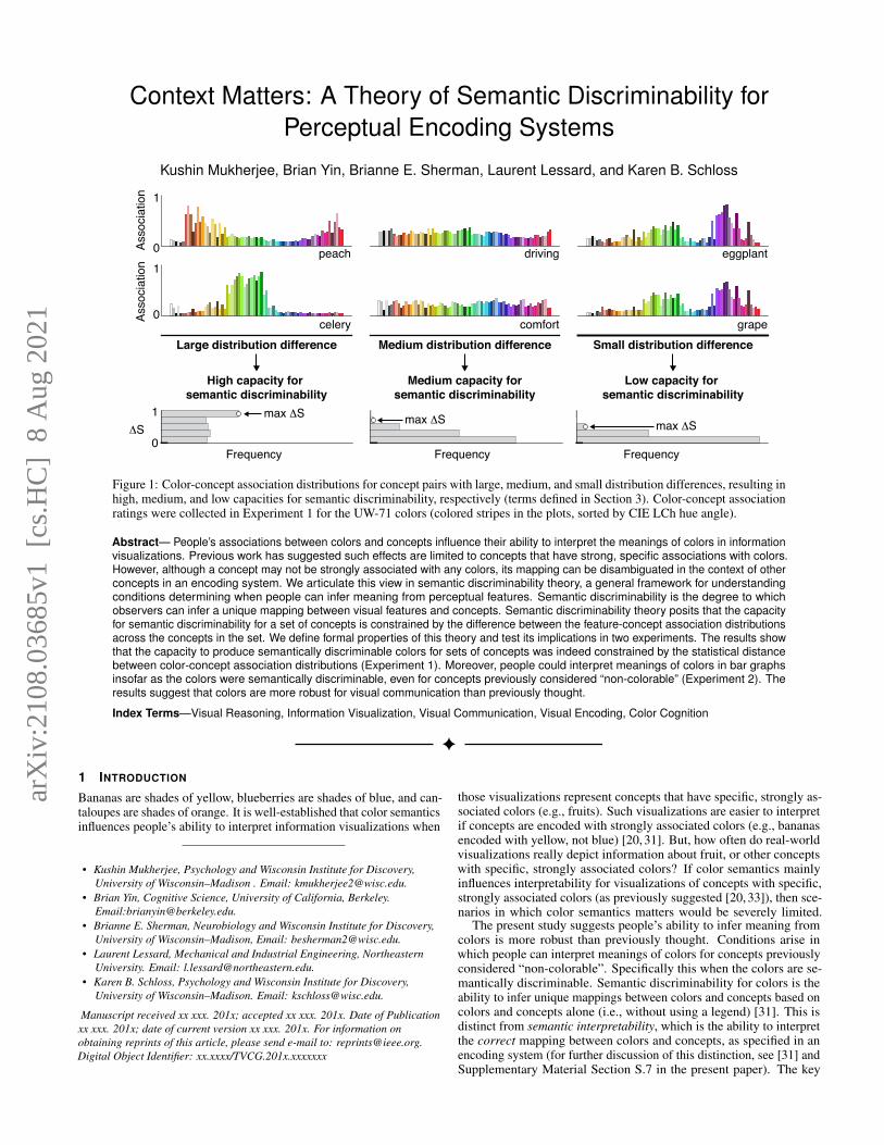
Figure 1: Color-concept association distributions for concept pairs with large, medium, and small distribution differences, resulting inhigh, medium, and low capacities for semantic discriminability, respectively (terms defined in Section 3). Color-concept associationratings were collected in Experiment 1 for the UW-71 colors (colored stripes in the plots, sorted by CIE LCh hue angle).
Abstract— People’s associations between colors and concepts influence their ability to interpret the meanings of colors in informationvisualizations. Previous work has suggested such effects are limited to concepts that have strong, specific associations with colors.However, although a concept may not be strongly associated with any colors, its mapping can be disambiguated in the context of otherconcepts in an encoding system. We articulate this view in semantic discriminability theory, a general framework for understandingconditions determining when people can infer meaning from perceptual features. Semantic discriminability is the degree to whichobservers can infer a unique mapping between visual features and concepts. Semantic discriminability theory posits that the capacityfor semantic discriminability for a set of concepts is constrained by the difference between the feature-concept association distributionsacross the concepts in the set. We define formal properties of this theory and test its implications in two experiments. The results showthat the capacity to produce semantically discriminable colors for sets of concepts was indeed constrained by the statistical distancebetween color-concept association distributions (Experiment 1). Moreover, people could interpret meanings of colors in bar graphsinsofar as the colors were semantically discriminable, even for concepts previously considered “non-colorable” (Experiment 2). Theresults suggest that colors are more robust for visual communication than previously thought.
Index Terms—Visual Reasoning, Information Visualization, Visual Communication, Visual Encoding, Color Cognition
1 INTRODUCTION
Bananas are shades of yellow, blueberries are shades of blue, and can-taloupes are shades of orange. It is well-established that color semanticsinfluences people’s ability to interpret information visualizations when
• Kushin Mukherjee, Psychology and Wisconsin Institute for Discovery,University of Wisconsin–Madison . Email: [email protected].
• Brian Yin, Cognitive Science, University of California, Berkeley.Email:[email protected].
• Brianne E. Sherman, Neurobiology and Wisconsin Institute for Discovery,University of Wisconsin–Madison, Email: [email protected].
• Laurent Lessard, Mechanical and Industrial Engineering, NortheasternUniversity. Email: [email protected].
• Karen B. Schloss, Psychology and Wisconsin Institute for Discovery,University of Wisconsin–Madison. Email: [email protected].
Manuscript received xx xxx. 201x; accepted xx xxx. 201x. Date of Publicationxx xxx. 201x; date of current version xx xxx. 201x. For information onobtaining reprints of this article, please send e-mail to: [email protected] Object Identifier: xx.xxxx/TVCG.201x.xxxxxxx
those visualizations represent concepts that have specific, strongly as-sociated colors (e.g., fruits). Such visualizations are easier to interpretif concepts are encoded with strongly associated colors (e.g., bananasencoded with yellow, not blue) [20, 31]. But, how often do real-worldvisualizations really depict information about fruit, or other conceptswith specific, strongly associated colors? If color semantics mainlyinfluences interpretability for visualizations of concepts with specific,strongly associated colors (as previously suggested [20, 33]), then sce-narios in which color semantics matters would be severely limited.
The present study suggests people’s ability to infer meaning fromcolors is more robust than previously thought. Conditions arise inwhich people can interpret meanings of colors for concepts previouslyconsidered “non-colorable”. Specifically this when the colors are se-mantically discriminable. Semantic discriminability for colors is theability to infer unique mappings between colors and concepts based oncolors and concepts alone (i.e., without using a legend) [31]. This isdistinct from semantic interpretability, which is the ability to interpretthe correct mapping between colors and concepts, as specified in anencoding system (for further discussion of this distinction, see [31] andSupplementary Material Section S.7 in the present paper). The key
arX
iv:2
108.
0368
5v1
[cs
.HC
] 8
Aug
202
1
question is, what determines whether it is possible to select semanticallydiscriminable colors for a set of concepts?
We address this question in semantic discriminability theory, a newtheory on constraints for generating semantically discriminable per-ceptual features for encoding systems that map perceptual features toconcepts. We tested two hypotheses that arise from the theory. First,the capacity to create semantically discriminable color palettes for aset of concepts depends on the difference in color-concept associa-tion distributions between those concepts, independent of propertiesof the concepts in isolation (Experiment 1). Second, people can ac-curately interpret mappings between colors and concepts for conceptspreviously considered “non-colorable,” to the extent that the colorsare semantically discriminable (Experiment 2). We focus on color inthis study, but present the theory in terms of perceptual features moregenerally because of its potential to extend to other types of visualfeatures (e.g., shape, orientation, visual texture) and features in otherperceptual modalities (e.g., sound, odor, touch).
Contributions. This paper makes the following contributions:(1) We define semantic discriminability theory (Section 3) and testhypotheses motivated by the theory in Experiments 1 and 2 (Sections4-5), and (2) We define a new metric for operationalizing distributiondifference between sets of more than two concepts (Section 3.2) andshow that it predicts capacity for semantic discriminability (Section 4).
2 BACKGROUND
Color is a strong cue for signaling meaning in nature and some ar-gue that color vision evolved for the purpose of visual communica-tion [7,8,12,14,39]. Historically, discussions on the role of color seman-tics in information visualization have tended to focus on few cases oftypical associations (e.g., red for hot, green for grass) [5, 28, 34]. Morerecent work has sought to understand the potential and limitations ofusing color to communicate meaning in visualizations [1, 2, 20, 31–33].The semantics of color in visualizations operates on two main levels:meaning of a color palette as a whole [1, 2, 15] and meaning of theindividual colors in a palette [20, 31–33]. We focus on meanings ofindividual colors because that is central to the present work. Peoplehave expectations about how colors will map onto concepts, and visual-izations that violate those expectations are harder to interpret, even ifthere is a legend [20, 30, 35]. Thus, understanding these expectations isimportant for optimizing palette design for visual communication.
2.1 Color-concept associationsColor-concept associations represent the degree to which individualcolors are associated with individual concepts. Color-concept asso-ciations can be quantified using various methods, including humanjudgments [16, 17, 25, 27, 31, 32, 38], image statistics [20–22, 27, 33],and natural language corpora [13, 33]. Some approaches focused onidentifying the strongest, or strongest few colors associated with aconcept [11, 13, 33], but color-concept associations can be treated asa continuous property over all possible colors in a perceptual colorspace [20–22, 27, 29]. When quantifying color-concept associationsover all of color space, researchers typically bin or sub-sample parts ofthe space to make measurements computationally tractable. An assump-tion is that the space is continuous, so nearby colors will have similarassociations. Figure 1 shows examples of color-concept associationsfor colors systematically sampled over CIELAB space (see Experiment1), plotted over one dimension (sorted by hue angle and chroma withachromatics at the beginning of the list). Perceptual color spaces arethree-dimensional so this representation does not necessarily positionperceptually similar colors in close proximity [41], but it does high-light how some concepts, like peach and celery, have specific, stronglyassociated colors, whereas other concepts, like driving and comfort,are more uniform (Figure 1). We refer to this ‘peakiness’ property asspecificity of the color-concept association distributions.1
1Specificity is similar to color diagnosticity [37], but color diagnosticityconcerns whether a concept has a single strongly associated color [37], andspecificity concerns the degree to which a concept is associated with some colorsmore than others in a color-concept association distribution.
Questions remain concerning how color concept-associations areformed, but many have suggested that they are learned through experi-ences [10, 16, 27, 38, 40] and may be continually updated through eachnew experience in the world [29]. Some color-concept associationsare shared cross-culturally, and others are subject to cultural differ-ences [16,17,38]. We will consider the role of cultural differences withrespect to the present work in the General Discussion.
Color-concept associations contribute to people’s expectations aboutthe meanings of colors in information visualizations [20, 31, 32], calledinferred mappings. However, associations and inferred mappings arenot the same, and sometimes they conflict [32]. We explain this pointin Section 2.3 on assignment inference.
2.2 Colorabilty scoresSome have suggested that the effectiveness of colors for encoding mean-ing is limited to concepts that have strong associations with particularcolors [18, 20, 33]. This idea is explained by invoking colorabilityscores, which broadly measure how strongly individual concepts can bemapped to specific colors. Generally, concepts with specific, stronglyassociated colors (‘banana’) are thought to be colorable, whereas moreabstract concepts, such as ‘comfort’ or ‘leisure’, that lack such stronglyassociated colors, have been called non-colorable.
Different methods have been used to define colorability. Lin etal. [20] quantified colorability by having participants assign colorsto concepts and rate the strength of the assignment. The mean ofthese ratings over all colors for a concept was used to generate a col-orability score for that concept. They found that participants werebetter at interpreting bar charts when palettes were optimized for colorsemantics compared to when palettes had the default Tableau color or-dering, but this benefit was mostly limited to highly colorable concepts.Setlur and Stone [33] quantified colorability with an automated method,using Google N-grams to determine how frequently a concept wordco-occurred with basic color terms [3] in linguistic corpora. They thenexcluded concepts they found to be non-colorable when developingmethods to optimize palette design.
These prior studies highlighted the importance of considering colorsemantics in palette design. However, our work suggests that restrictingnotions of colorability to concepts in isolation may have led to underes-timating people’s ability to infer meaning from colors in visualizations.
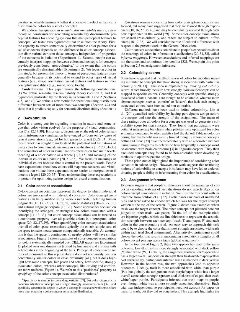
2.3 Assignment inferenceEvidence suggests that people’s inferences about the meanings of col-ors in encoding systems of visualizations do not merely depend oncolor-concept associations in isolation. We illustrate this point with anexample from Schloss et al. [32]. Participants saw pairs of unlabeledbins and were asked to choose which bin was for the target conceptwritten at the top of the screen. Figure 2 shows two examples whentrash was the target concept. The other concept, not pictured here butjudged on other trials, was paper. To the left of the example trialsare bipartite graphs, which use line thickness to represent the associa-tion strength between each concept (trash, T, and paper, P) and eachcolor in the corresponding trial. An easy way to approach this taskwould be to choose the color that is most strongly associated with trashwithin each trial (local assignment). Alternatively, participants couldchoose the color that results in maximizing association strengths of allcolor-concept pairings across trials (global assignment).
In the top row of Figure 2, these two approaches lead to the sameoutcome. Locally, trash is more strongly associated with dark yellow(Y) than white (W). Globally, the assignment trash-yellow/paper-whitehas a larger overall association strength than trash-white/paper-yellow.Not surprisingly, participants inferred trash is mapped to dark yellow.However, in the bottom row, the two approaches lead to oppositeoutcomes. Locally, trash is more associated with white than purple(Pu), but globally the assignment trash-purple/paper-white has a largeroverall association strength (greater total thickness of edges) than trash-white/paper-purple. Participants inferred that trash maps to purple,even though white was a more strongly associated alternative. Eachtrial was independent, so participants need not account for paper ontrials for trash, but they did so nonetheless. This example highlights the
ConsistentInferred mappingStronger associate
ConflictInferred mapping
Stronger associate
Concepts
Colors
T P
Pu W
TRASH
TRASH
T P
Y W
Concepts
Colors
Figure 2: Distinction between color-concept associations and inferredmappings (figure based on [32]). Left: Bipartite graphs show color-concept association strengths for concepts trash (T) and paper (P) withcolors dark yellow (Y), white (W), and purple (Pu) (thicker edgesconnecting concepts and colors indicate stronger associations). Right:example trials where participants infer which color maps to trash.
important distinction between color-concept associations for a singlecolor and concept, and inferred mappings between a color and conceptin the context of an encoding system.
Schloss et al. [32] called this process of inferring mappings betweencolors and concepts assignment inference because it is analogous to anassignment problem in optimization. In assignment problems, everypossible pairing of items in one category (e.g., colors) i and anothercategory (e.g., concepts) j is given a numerical merit score mi j. Here,let’s assume that larger scores indicate a more desirable pairing, butthat is not always true (e.g., to optimize delivery route efficiency, meritmight be delivery time and smaller scores would be better). Solving anassignment problem means finding the pairing of items that maximizes(or minimizes) the sum of the merit scores of all chosen pairs [6,19,23].
Although assignment inference is analogous to assignment prob-lems, they are not the same. Assignment problems have deterministicresults, whereas assignment inference is stochastic—inferred map-pings can vary among individuals and even within individuals overtime. This stochasticity can be explained in terms of noise in people’scolor-concept associations affecting the outcome of assignments inassignment inference, depending on whether assignments are robust orfragile [31]. In robust assignments, adding noise to the system (e.g.,perturbing the color-concept association strengths) has no effect onthe outcome, but in fragile assignments adding noise can change theoutcome of the assignment.
The robustness of an assignment in assignment inference can beunderstood as semantic discriminability—the ability for people to infera unique mapping between colors and concepts [31]. Evidence sug-gests that semantic discriminability predicts people’s ability to interpretcolors in encoding systems, independent of that predicted by perceptualdiscriminability and color-concept associations in isolation [31]. We de-scribe ways of operationalizing semantic discriminability in Section 3.2as they pertain to the present study.
So far, we focused on encoding systems with two concepts andcolors, and implied that merit mi j in assignment inference is color-concept association strength (Figure 2). However, there are otherpossible ways to define merit, especially when there are more thantwo colors and concepts, as in the present study. Schloss et al. [32]sought to understand which merit people use in assignment inferenceto study (1) how humans infer meaning from colors, and (2) how todesign palettes that match people’s expectations, making palettes moreinterpretable. To approach this goal, they created two definitions ofmerit. The isolated merit function simply uses association strengthsbetween items i and j, mi j := ai j. The balanced merit function isdefined as
mi j := ai j−maxk 6= j
aik. (1)
The balanced merit score for a given color-concept pair is the associa-tion strength for that pair, minus the association strength between thatcolor and the next most strongly associated concept. In order for mi jto be large, color i should be strongly associated with concept j andweakly associated with all other concepts. (Note: in the case of twoconcepts and colors these two definitions reduce to the same outcome.)
Next, they generated color palettes using an assignment problemunder each definition, with human color-concept association ratingsas the input. Finally, they presented different participants with thosepalettes in the form of six unlabeled colored bins. Participants inferredwhich bin was for each of six objects: paper, plastic, trash, metal,compost, and glass. Responses were scored as “correct” interpretationsif they matched the encoded mapping. Encoded mappings can beproduced in different ways, including by designers, software defaults,or optimization algorithms [20, 31, 32]. Here, they were determined bythe optimal assignments in assignment problems used to generate thepalettes. The logic was that participants would be better at interpretingpalettes generated using a merit function that more closely matchedmerit in assignment inference. Performance was better for the palettegenerated using the balanced merit function, which suggests that thiswas the function that better captured merit in assignment inference.Thus, we use balanced merit in the present study.
Balanced merit can lead to unexpected assignments. For example,the bin for plastic was assigned a red color, even though red was weaklyassociated with plastic, because that color was more associated withplastic than with any of the other concepts. Thus, the assignment ofplastic–red was interpretable. Given that weakly associated colorscan prove useful when designing encoding systems, approaches thatfocus only on the top associates may be limited [11]. It is important toquantify associations between concepts and a large range of colors, notjust the top few associates, when optimizing palette design [27].
3 SEMANTIC DISCRIMINABILITY THEORY
Semantic discriminability theory characterizes the ability to generatesemantically discriminable perceptual features for encoding a set ofconcepts. We begin with some key definitions.
Concept set: This is the set of all concepts that are represented inan encoding system. These concepts could refer to any information thatis categorical (e.g., food, weather, activities, places, and animals). Welabel concepts in the concept set using the index j ∈ {1,2, . . . ,n}.
Feature source: This is the set of all possible instances of a featuretype. Perceptual color spaces (e.g., CIELAB) are well-defined featuresources for color, as they represent all colors humans can perceive [41].
Feature library: This is a subset of candidate features from thefeature source used in an encoding system. For example, the Tableau 20colors or UW-58 colors [27] are feature libraries if design is constrainedto those groups of colors. We focus on a feature library defined overcolor, but they can be defined over any type of perceptual feature (e.g.,shapes, sizes, textures). We label features in the feature library usingthe index i ∈ {1,2, . . . ,N}.
Feature set: This is a subset of features from the feature library,selected to encode a concept set. Feature sets can be constructed fromany type of perceptual features (e.g., colors, shapes, sizes) [4]. Forcolors, they are called “palettes.” If there are n concepts, then thefeature set should contain n features.
3.1 Feature-concept association distributions
Feature-concept association distributions represent the degree to whicha given concept is associated with each feature in a feature library(see Figure S.5A. in the Supplementary Material). For color, these arecolor-concept association distributions. Feature-concept associationdistributions can be described as raw association values over the featurelibrary (e.g., mean ratings, pixel counts, word counts). In this case, wewrite ai j to denote the association between feature i ∈ {1, . . . ,N} andconcept j ∈ {1, . . . ,n}. For each concept j, we also define normalizedassociations p j(·) as
p j(i) :=ai j
∑Nk=1 ak j
for: i ∈ {1, . . . ,N}. (2)
The list[p j(1) p j(2) · · · p j(N)
]can be interpreted as a discrete
probability distribution over features in the feature library.We now define useful properties and operations related to feature-
concept association distributions.
3.1.1 SpecificitySpecificity is the degree to which a concept has strong, specific associa-tions with features over the feature library. For color, specificity refersto the ‘peakiness’ of a color-concept association distribution. Conceptscan have strong color associations that are concentrated in one partof color space (e.g., reds for concepts like raspberry) or divided overdifferent parts of color space (e.g., reds and greens for watermelon) [27].Thus, we quantify specificity using entropy of the distribution, whichcaptures how ‘flat’ vs. ‘peaky’ a distribution is, regardless of how manypeaks there are.
Entropy for a feature-concept association distribution is defined as:
H j :=−N
∑i=1
p j(i) log p j(i). (3)
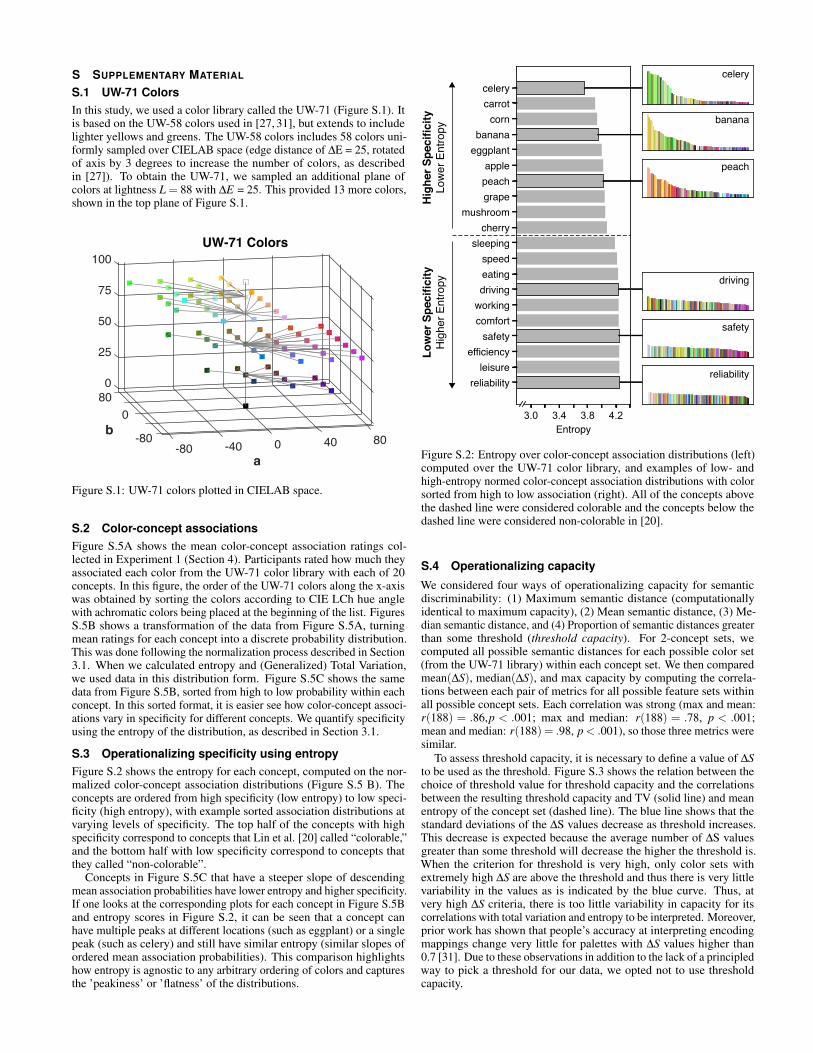
If all features in the feature library are equally associated with con-cept j, the distribution p j will be uniform, entropy will be high, andspecificity will be low. If a concept j is strongly associated with somefeatures and not others, then entropy will be lower and specificity willbe higher. This property of color-concept association distributionsaligns with previous measures of colorability [20, 33] (see Figure S.2in the Supplementary Material).
Mean entropy of a concept set is the mean of the entropy of allconcepts in the set: Hµ := 1
n (H1 + · · ·+Hn).
3.1.2 Distribution differenceWe quantify distribution difference between concepts by comparingtheir normalized feature-concept associations.
Total variation (TV) is what we use when comparing two concepts,say j1 and j2. TV is defined as follows.
TV( j1, j2) :=12
N
∑i=1
∣∣p j1(i)− p j2(i)∣∣ . (4)
TV ranges between 0 and 1, where TV = 0 means the two distributionsare identical, and TV = 1 means they are disjoint (for each feature i,either p j1(i) or p j2(i) must be zero).
Generalized total variation (GTV) is a generalization of TV thatwe defined for cases when more than two concepts must be compared,say j1, . . . , jk. We define GTV as follows.
GTV( j1, . . . , jk) :=−1+N
∑i=1
max(p j1(i), p j2(i), . . . , p jk (i)). (5)
In the case where k = 2, GTV reduces to TV. In other words,GTV( j1, j2) = TV( j1, j2). For details on the motivation behind ourdefinition of GTV, see the Supplementary Material, Section S.6.
3.1.3 Structure-agnostic propertyThe notions of entropy, TV, and GTV are agnostic to intrinsic structureof the feature source. For example, perceptual color spaces are struc-tured according to perceptual similarity, but entropy of a color-conceptdistribution depends on the fraction of the colors that are highly asso-ciated with the concept, regardless of perceptual similarity. We chosestructure-agnostic metrics for specificity and distribution difference sothat semantic discriminability theory could readily generalize to featuresources with less well-defined metric spaces (e.g., shape, texture, odor).
3.2 Semantic discriminabilityAs described in Section 2.3, semantic discriminability of perceptualfeatures is the ability to infer a unique mapping between features andconcepts. It is reflected in the degree to which inferred mappings varyamong individuals or within individuals between trials. We model thisvariability by treating feature-concept associations as random variables.Rather than solving an assignment problem using the mean ai j values,we look at the probability of the likeliest assignment, where probabilityis computed with respect to uncertainty in the ai j. We now make thisnotion more precise.
Semantic distance is a way to operationalize semantic discrim-inability in the case where there are n = 2 features and concepts [31].
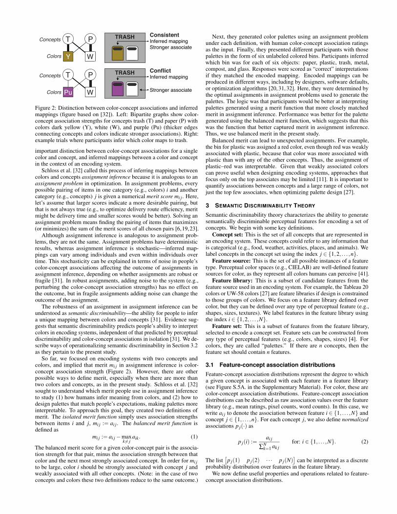
Figure 3 illustrates an example in which we have concepts {M,W} andcolors {1,2}. The color-concept associations between all possible pairsare x1, . . . ,x4, as shown in Figure 3. We assume each xk is normallydistributed with mean xk equal to the corresponding ai j and standarddeviation σk = 1.4 · xk(1− xk), which was found to be a good fit toexperimental data [31]. The outcome of the assignment problem isdetermined by the quantity ∆x := x1− x2 + x3− x4. The optimal as-signment is: (M-1 and W-2 if ∆x > 0) and (M-2 and W-1 if ∆x < 0).Semantic distance is defined by the equation
∆S = |Prob(∆x > 0)−Prob(∆x < 0)|. (6)
Since the xk are assumed to be normally distributed, so is ∆x, and theprobabilities in (6) can be computed analytically:
Prob(∆x > 0) = Φ
(x1 + x4)− (x2 + x3)√σ2
1 +σ22 +σ2
3 +σ24
, (7)
and Prob(∆x < 0) = 1−Prob(∆x > 0), where Φ(·) is the cumulativedistribution function (cdf) of the standard normal distribution. When ∆Sis close to 0, ∆x has a similar probability of being positive or negative,so the assignment is fragile. When ∆S is close to 1, ∆x is almost alwayspositive or almost always negative, so the assignment is robust. Thisnotion of semantic distance can be used even when the features are notcolors, by replacing the color-concept associations with feature-conceptassociations, and adjusting the formula for σk as appropriate.
-2 -1 0 1 2
Distribution of Δx = (x1 + x4) – (x2 + x3)
Association Rating
Pro
b.
Den
sity
Pro
babi
lity
Den
sity
Concept WConcept MConcept M Concept W
x1 x3x2x4+ +–( ) ( )
Color 1 Color 2 Color 2 Color 1
M W
1
x1 x2 x4x3
2
M W
1
x1 x2 x4x3
2Prob(Δx < 0)
Prob(Δx > 0)
Figure 3: Diagram from [31] that shows how association ratings be-tween concepts {M,W} and colors {1,2} produce a distribution for ∆x.Semantic distance is the absolute difference of the area under the curveto the left and right of zero.
Generalized semantic distance is an extension of semantic dis-tance to the case where there are n > 2 features and concepts. In thiscase, there will be n! (n factorial) possible assignments. We definegeneralized semantic distance in a manner analogous to semantic dis-tance; we label the feature-concept associations between all possiblepairs as x1,x2, . . . ,xn2 and assume they are normally distributed randomvariables.2 In this more complicated scenario, the assignment is notdetermined by a simple quantity such as ∆x and no formula analogousto (7) exists to determine the assignment. Instead, we use the followingMonte Carlo approach.
1. Sample x1, . . . ,xn2 from the distribution of merit scores2 and solvean assignment problem using the sampled merit scores.
2. Repeat step 1 a large number of times and count the number oftimes each distinct assignment occurs. Let p be the proportion oftimes that the most frequent assignment occurred. Since there aren! possible assignments, we must have 1
n! ≤ p≤ 1.2Here, we use color-concept association ratings, so we assume the xk are
distributed with the same σk used to define semantic distance [31]. In principle,the distributions of the xk can be changed to suit other cases beyond color.
Asso
c.As
soc.
Asso
c.As
soc.
Asso
c.
Freq. Freq. Freq.
Freq.Color Library
Color Library
Color Library
Color Library
Color Library
Color Library
Freq. Freq.
Hig
her
Cap
acity
Low
er
Cap
acity
ΔS = .99
ΔS ΔS ΔS
ΔSΔSΔS
ΔS = .56
ΔS = .86
ΔS = 0
ΔS = .98
ΔS = 0
A BA B
AB
A
BA B
BA
BA
BA
BA
BA
BA
max ΔS
1
0
max ΔS
Asso
c.
AB
1
0
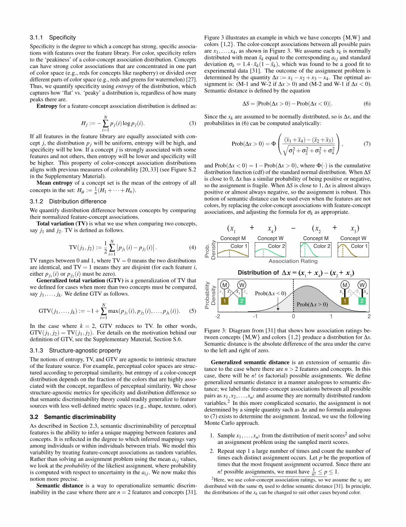
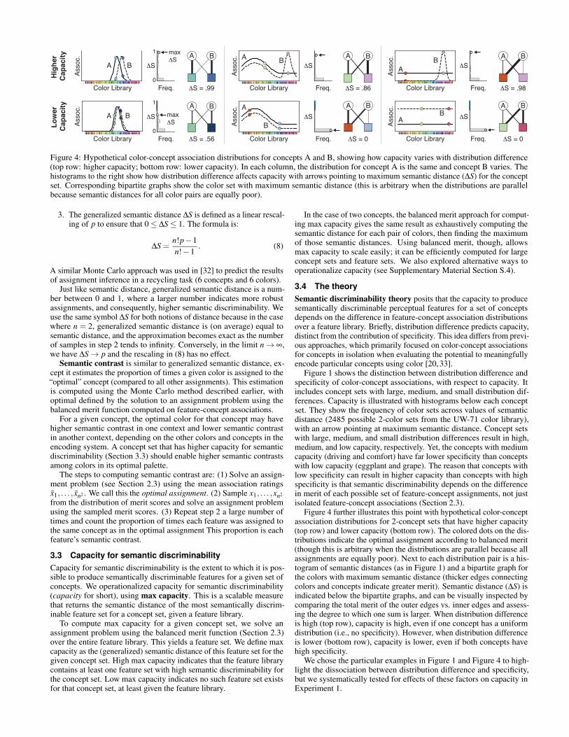
Figure 4: Hypothetical color-concept association distributions for concepts A and B, showing how capacity varies with distribution difference(top row: higher capacity; bottom row: lower capacity). In each column, the distribution for concept A is the same and concept B varies. Thehistograms to the right show how distribution difference affects capacity with arrows pointing to maximum semantic distance (∆S) for the conceptset. Corresponding bipartite graphs show the color set with maximum semantic distance (this is arbitrary when the distributions are parallelbecause semantic distances for all color pairs are equally poor).
3. The generalized semantic distance ∆S is defined as a linear rescal-ing of p to ensure that 0≤ ∆S≤ 1. The formula is:
∆S =n!p−1n!−1
. (8)
A similar Monte Carlo approach was used in [32] to predict the resultsof assignment inference in a recycling task (6 concepts and 6 colors).
Just like semantic distance, generalized semantic distance is a num-ber between 0 and 1, where a larger number indicates more robustassignments, and consequently, higher semantic discriminability. Weuse the same symbol ∆S for both notions of distance because in the casewhere n = 2, generalized semantic distance is (on average) equal tosemantic distance, and the approximation becomes exact as the numberof samples in step 2 tends to infinity. Conversely, in the limit n→ ∞,we have ∆S→ p and the rescaling in (8) has no effect.
Semantic contrast is similar to generalized semantic distance, ex-cept it estimates the proportion of times a given color is assigned to the“optimal” concept (compared to all other assignments). This estimationis computed using the Monte Carlo method described earlier, withoptimal defined by the solution to an assignment problem using thebalanced merit function computed on feature-concept associations.
For a given concept, the optimal color for that concept may havehigher semantic contrast in one context and lower semantic contrastin another context, depending on the other colors and concepts in theencoding system. A concept set that has higher capacity for semanticdiscriminability (Section 3.3) should enable higher semantic contrastsamong colors in its optimal palette.
The steps to computing semantic contrast are: (1) Solve an assign-ment problem (see Section 2.3) using the mean association ratingsx1, . . . , xn2 . We call this the optimal assignment. (2) Sample x1, . . . ,xn2
from the distribution of merit scores and solve an assignment problemusing the sampled merit scores. (3) Repeat step 2 a large number oftimes and count the proportion of times each feature was assigned tothe same concept as in the optimal assignment This proportion is eachfeature’s semantic contrast.
3.3 Capacity for semantic discriminabilityCapacity for semantic discriminability is the extent to which it is pos-sible to produce semantically discriminable features for a given set ofconcepts. We operationalized capacity for semantic discriminability(capacity for short), using max capacity. This is a scalable measurethat returns the semantic distance of the most semantically discrim-inable feature set for a concept set, given a feature library.
To compute max capacity for a given concept set, we solve anassignment problem using the balanced merit function (Section 2.3)over the entire feature library. This yields a feature set. We define maxcapacity as the (generalized) semantic distance of this feature set for thegiven concept set. High max capacity indicates that the feature librarycontains at least one feature set with high semantic discriminability forthe concept set. Low max capacity indicates no such feature set existsfor that concept set, at least given the feature library.
In the case of two concepts, the balanced merit approach for comput-ing max capacity gives the same result as exhaustively computing thesemantic distance for each pair of colors, then finding the maximumof those semantic distances. Using balanced merit, though, allowsmax capacity to scale easily; it can be efficiently computed for largeconcept sets and feature sets. We also explored alternative ways tooperationalize capacity (see Supplementary Material Section S.4).
3.4 The theorySemantic discriminability theory posits that the capacity to producesemantically discriminable perceptual features for a set of conceptsdepends on the difference in feature-concept association distributionsover a feature library. Briefly, distribution difference predicts capacity,distinct from the contribution of specificity. This idea differs from previ-ous approaches, which primarily focused on color-concept associationsfor concepts in isolation when evaluating the potential to meaningfullyencode particular concepts using color [20, 33].
Figure 1 shows the distinction between distribution difference andspecificity of color-concept associations, with respect to capacity. Itincludes concept sets with large, medium, and small distribution dif-ferences. Capacity is illustrated with histograms below each conceptset. They show the frequency of color sets across values of semanticdistance (2485 possible 2-color sets from the UW-71 color library),with an arrow pointing at maximum semantic distance. Concept setswith large, medium, and small distribution differences result in high,medium, and low capacity, respectively. Yet, the concepts with mediumcapacity (driving and comfort) have far lower specificity than conceptswith low capacity (eggplant and grape). The reason that concepts withlow specificity can result in higher capacity than concepts with highspecificity is that semantic discriminability depends on the differencein merit of each possible set of feature-concept assignments, not justisolated feature-concept associations (Section 2.3).
Figure 4 further illustrates this point with hypothetical color-conceptassociation distributions for 2-concept sets that have higher capacity(top row) and lower capacity (bottom row). The colored dots on the dis-tributions indicate the optimal assignment according to balanced merit(though this is arbitrary when the distributions are parallel because allassignments are equally poor). Next to each distribution pair is a his-togram of semantic distances (as in Figure 1) and a bipartite graph forthe colors with maximum semantic distance (thicker edges connectingcolors and concepts indicate greater merit). Semantic distance (∆S) isindicated below the bipartite graphs, and can be visually inspected bycomparing the total merit of the outer edges vs. inner edges and assess-ing the degree to which one sum is larger. When distribution differenceis high (top row), capacity is high, even if one concept has a uniformdistribution (i.e., no specificity). However, when distribution differenceis lower (bottom row), capacity is lower, even if both concepts havehigh specificity.
We chose the particular examples in Figure 1 and Figure 4 to high-light the dissociation between distribution difference and specificity,but we systematically tested for effects of these factors on capacity inExperiment 1.
4 EXPERIMENT 1Experiment 1 tested the hypothesis that capacity for semantic dis-criminability is predicted by distribution difference, independent ofspecificity. We first collected color-concept association data fromhuman participants, and used those data to calculate capacity, dis-tribution difference, and specificity. We then tested our hypothe-sis on 2-concept sets (Section 4.2.1) and 4-concepts sets (Section4.2.2). Semantic discriminability predicts people’s ability to interpretpalettes in visualizations [31], so our modeling approach for under-standing capacity for semantic discriminability should have implica-tions for interpretability. The code and data for all experiments is at:https://github.com/SchlossVRL/sem_disc_theory.
4.1 Methods4.1.1 Participants185 undergraduates participated for credit in Introductory Psychology(mean age =18.66, 99 females, 86 males, gender provided throughfree-response). All gave informed consent and the UW–Madison IRBapproved the protocol. Color vision was assessed by asking participantsif they had difficulty distinguishing between colors relative to the aver-age person and if they considered themselves colorblind. Participantswere excluded if they answered yes to either (5 excluded).
4.1.2 Design, Displays, and ProcedureParticipants judged the association between each of 71 colors and eachof 20 concepts. The colors were the UW-71 color library, an extensionof the UW-58 colors [31], see Supplementary Material for details andTable S.1 for CIELAB coordinates.3 The concepts were from Lin etal. [20], including 5 concepts in each of four concept categories (fruits,vegetables, activities, and properties) (Table 1). Participants wererandomly assigned to one of four categories (fruits n = 46, vegetablesn = 45, activities n = 45, properties n = 44). They judged all colors forall five concepts within their assigned category (71 colors × 5 concepts= 355 trials). Trials were presented in a blocked randomized design—all colors were presented in a random order for a given concept beforestarting the next concept, and concept order was also randomized.
The displays included the concept word centered at the top of thescreen (font-size: 24 pt, font-family: Lato) and colored square centeredbelow (80 px × 80 px). Below the colored square, was a line-markslider scale (400 px long), with the left end labeled “not at all” and theright end labeled “very much” and the center marked with a vertical line(3 px wide and 32 px tall). The background was gray (CIE IlluminantD65, x = .3127, y = .3290, Y = 10 cd/m2), so that very dark colors(e.g., black) and very light colors (e.g., white) could be seen against thebackground. Data were recorded in pixel units, and scaled to range from0-1. Displays were generated using the jsPsych JavaScript library [9],presented on participants’ personal devices.
Participants were told they would see a set of concepts and seriesof colors, one concept and color at a time. Their task was to rate howmuch they associated the color with the concept by moving the slideron the scale from “not at all” to “very much”, and clicking “next” tocontinue. Before beginning, they were shown a list of all conceptsand the UW-71 colors. They were asked to anchor the endpoints ofthe rating scale for each concept [26] by thinking about which colorthey associated the most/least with that concept, and considering thesecolors as representing the ends of the slider scale for that concept.During the experiment, ratings were blocked by concept, and after eachblock participants were told how many blocks remained.
4.2 Results and Discussion4.2.1 2-Concept setsWe began by calculating the mean color-concept association ratingsover participants. Next, for all k = 2 concepts out of the n= 20 concepts
3We converted CIELAB to RGB using MATLAB’s lab2rgb function, whichmakes assumptions about monitor characteristics, so the colors were not exactrenderings of CIELAB coordinates. Without calibration, the colors rendered byRGB coordintes may vary across monitors, but using a fixed correspondencebetween D65 CIELAB and RGB can approximate intended colors online [36].
Table 1: Full set of concepts in Experiment 1 (first four columns ofconcepts were used in Experiment 2).
Category Concepts
Fruits peach cherry grape banana appleVegetables corn carrot eggplant celery mushroomActivities working leisure sleeping driving eatingProperties efficiency speed safety comfort reliability
−4 −3 −2 −1 0
log(normalized TV)
0.0
0.2
0.4
0.6
0.8
1.0
2-C
once
pt S
ets
Cap
acity
max
ΔS
r = .93
−6 −5 −4 −3 −2
log(1 − normalized Hμ)
r = .82
−3 −2 −1
log(normalized GTV)
0.0
0.2
0.4
0.6
0.8
1.0
4-C
once
pt S
ets
Cap
acity
max
ΔS
r = .74
−6 −5 −4 −3 −2
log(1 − normalized Hμ)
r = .61
Distribution Difference Mean Specificity
Distribution Difference Mean Specificity
A
B
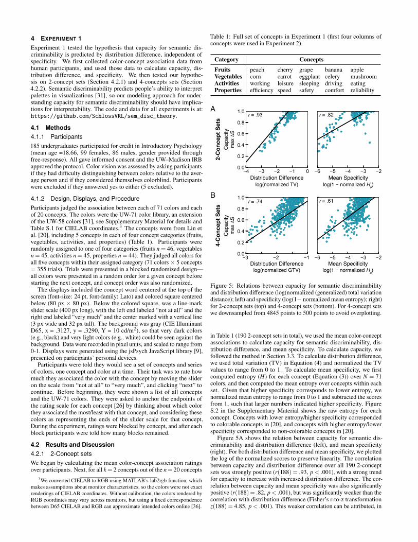
Figure 5: Relations between capacity for semantic discriminabilityand distribution difference (log(normalized (generalized) total variationdistance); left) and specificity (log(1− normalized mean entropy); right)for 2-concept sets (top) and 4-concept sets (bottom). For 4-concept setswe downsampled from 4845 points to 500 points to avoid overplotting.
in Table 1 (190 2-concept sets in total), we used the mean color-conceptassociations to calculate capacity for semantic discriminability, dis-tribution difference, and mean specificity. To calculate capacity, wefollowed the method in Section 3.3. To calculate distribution difference,we used total variation (TV) in Equation (4) and normalized the TVvalues to range from 0 to 1. To calculate mean specificity, we firstcomputed entropy (H) for each concept (Equation (3)) over N = 71colors, and then computed the mean entropy over concepts within eachset. Given that higher specificity corresponds to lower entropy, wenormalized mean entropy to range from 0 to 1 and subtracted the scoresfrom 1, such that larger numbers indicated higher specificity. FigureS.2 in the Supplementary Material shows the raw entropy for eachconcept. Concepts with lower entropy/higher specificity correspondedto colorable concepts in [20], and concepts with higher entropy/lowerspecificity corresponded to non-colorable concepts in [20].
Figure 5A shows the relation between capacity for semantic dis-criminability and distribution difference (left), and mean specificity(right). For both distribution difference and mean specificity, we plottedthe log of the normalized scores to preserve linearity. The correlationbetween capacity and distribution difference over all 190 2-conceptsets was strongly positive (r(188) = .93, p < .001), with a strong trendfor capacity to increase with increased distribution difference. The cor-relation between capacity and mean specificity was also significantlypositive (r(188) = .82, p < .001), but was significantly weaker than thecorrelation with distribution difference (Fisher’s r-to-z transformationz(188) = 4.85, p < .001). This weaker correlation can be attributed, in
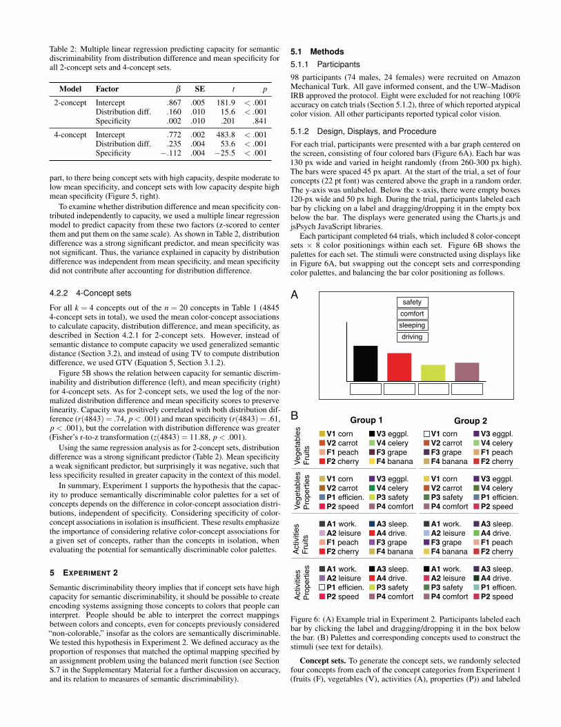
Table 2: Multiple linear regression predicting capacity for semanticdiscriminability from distribution difference and mean specificity forall 2-concept sets and 4-concept sets.
Model Factor β SE t p
2-concept Intercept .867 .005 181.9 < .001Distribution diff. .160 .010 15.6 < .001Specificity .002 .010 .201 .841
4-concept Intercept .772 .002 483.8 < .001Distribution diff. .235 .004 53.6 < .001Specificity −.112 .004 −25.5 < .001
part, to there being concept sets with high capacity, despite moderate tolow mean specificity, and concept sets with low capacity despite highmean specificity (Figure 5, right).
To examine whether distribution difference and mean specificity con-tributed independently to capacity, we used a multiple linear regressionmodel to predict capacity from these two factors (z-scored to centerthem and put them on the same scale). As shown in Table 2, distributiondifference was a strong significant predictor, and mean specificity wasnot significant. Thus, the variance explained in capacity by distributiondifference was independent from mean specificity, and mean specificitydid not contribute after accounting for distribution difference.
4.2.2 4-Concept sets
For all k = 4 concepts out of the n = 20 concepts in Table 1 (48454-concept sets in total), we used the mean color-concept associationsto calculate capacity, distribution difference, and mean specificity, asdescribed in Section 4.2.1 for 2-concept sets. However, instead ofsemantic distance to compute capacity we used generalized semanticdistance (Section 3.2), and instead of using TV to compute distributiondifference, we used GTV (Equation 5, Section 3.1.2).
Figure 5B shows the relation between capacity for semantic discrim-inability and distribution difference (left), and mean specificity (right)for 4-concept sets. As for 2-concept sets, we used the log of the nor-malized distribution difference and mean specificity scores to preservelinearity. Capacity was positively correlated with both distribution dif-ference (r(4843) = .74, p < .001) and mean specificity (r(4843) = .61,p < .001), but the correlation with distribution difference was greater(Fisher’s r-to-z transformation (z(4843) = 11.88, p < .001).
Using the same regression analysis as for 2-concept sets, distributiondifference was a strong significant predictor (Table 2). Mean specificitya weak significant predictor, but surprisingly it was negative, such thatless specificity resulted in greater capacity in the context of this model.
In summary, Experiment 1 supports the hypothesis that the capac-ity to produce semantically discriminable color palettes for a set ofconcepts depends on the difference in color-concept association distri-butions, independent of specificity. Considering specificity of color-concept associations in isolation is insufficient. These results emphasizethe importance of considering relative color-concept associations fora given set of concepts, rather than the concepts in isolation, whenevaluating the potential for semantically discriminable color palettes.
5 EXPERIMENT 2
Semantic discriminability theory implies that if concept sets have highcapacity for semantic discriminability, it should be possible to createencoding systems assigning those concepts to colors that people caninterpret. People should be able to interpret the correct mappingsbetween colors and concepts, even for concepts previously considered“non-colorable,” insofar as the colors are semantically discriminable.We tested this hypothesis in Experiment 2. We defined accuracy as theproportion of responses that matched the optimal mapping specified byan assignment problem using the balanced merit function (see SectionS.7 in the Supplementary Material for a further discussion on accuracy,and its relation to measures of semantic discriminability).
5.1 Methods5.1.1 Participants
98 participants (74 males, 24 females) were recruited on AmazonMechanical Turk. All gave informed consent, and the UW–MadisonIRB approved the protocol. Eight were excluded for not reaching 100%accuracy on catch trials (Section 5.1.2), three of which reported atypicalcolor vision. All other participants reported typical color vision.
5.1.2 Design, Displays, and Procedure
For each trial, participants were presented with a bar graph centered onthe screen, consisting of four colored bars (Figure 6A). Each bar was130 px wide and varied in height randomly (from 260-300 px high).The bars were spaced 45 px apart. At the start of the trial, a set of fourconcepts (22 pt font) was centered above the graph in a random order.The y-axis was unlabeled. Below the x-axis, there were empty boxes120-px wide and 50 px high. During the trial, participants labeled eachbar by clicking on a label and dragging/dropping it in the empty boxbelow the bar. The displays were generated using the Charts.js andjsPsych JavaScript libraries.
Each participant completed 64 trials, which included 8 color-conceptsets × 8 color positionings within each set. Figure 6B shows thepalettes for each set. The stimuli were constructed using displays likein Figure 6A, but swapping out the concept sets and correspondingcolor palettes, and balancing the bar color positioning as follows.
A
V1 cornV2 carrotF1 peachF2 cherry
V1 cornV2 carrotP1 efficien.P2 speed
V3 eggpl.V4 celeryF3 grapeF4 banana
V3 eggpl.V4 celeryP3 safetyP4 comfort
Group 1
Vege
tabl
es
Frui
tsAc
tiviti
esFr
uits
Activ
ities
Pr
oper
ties
Vege
tabl
esPr
oper
ties
B
A1 work.A2 leisureF1 peachF2 cherry
A3 sleep.A4 drive.F3 grapeF4 banana
A1 work.A2 leisureP1 efficien.P2 speed
A3 sleep.A4 drive.P3 safetyP4 comfort
V1 cornV2 carrotF3 grapeF4 banana
V1 cornV2 carrotP3 safetyP4 comfort
V3 eggpl.V4 celeryF1 peachF2 cherry
V3 eggpl.V4 celeryP1 efficien.P2 speed
Group 2
A1 work.A2 leisureF3 grapeF4 banana
A3 sleep.A4 drive.F1 peachF2 cherry
A1 work.A2 leisureP3 safetyP4 comfort
A3 sleep.A4 drive.P1 efficen.P2 speed
sleepingdriving
safetycomfort
Figure 6: (A) Example trial in Experiment 2. Participants labeled eachbar by clicking the label and dragging/dropping it in the box belowthe bar. (B) Palettes and corresponding concepts used to construct thestimuli (see text for details).
Concept sets. To generate the concept sets, we randomly selectedfour concepts from each of the concept categories from Experiment 1(fruits (F), vegetables (V), activities (A), properties (P)) and labeled
them 1-4 (Table 1, Figure 6B). We then tied pairs of concepts withineach category (e.g., V1-V2, V3-V4). We combined pairs of conceptssuch that all participants saw (1) vegetables with fruits, (2) vegetableswith properties, (3) activities with fruits, and (4) activities with proper-ties. Using this design, we created two groups of stimuli, divided overtwo groups of participants to reduce the number of trials for any oneparticipant. Group 1 saw sets of four concepts, with concepts 1 and 2in one category paired with concepts 1 and 2 in the other category (e.g.,V1-V2 with F1-F2), and sets of four concepts with concept 3 and 4 inone category paired with concepts 3 and 4 in the other category (e.g.,V3-V4 with F3-F4). Group 2 saw the opposite pairings (e.g., V1-V2with F3-F4, V3-V4 with F1-F2). Within this design, all participants saweach concept an equal number of times. Participants were randomlyassigned to Group 1 (n = 47) or Group 2 (n = 43).
Color palettes. For each concept set, we generated its color paletteusing the balanced merit function (Equation (1)) in an assignmentproblem. The resulting assignments determined the encoded mappingwe defined as “correct.” We used the balance merit function becauseprevious evidence suggested it aligns with the merit people use inassignment inference (see Section 2.3). Merit was computed overthe color-concept association data reported in Experiment 1 for all 71colors in the UW-71 library 4 The color palettes are shown in Figure 6B.The CIELAB coordinates for the palette colors can be found at https://github.com/SchlossVRL/sem_disc_theory. The graphs werepresented on a gray background approximating CIE Illuminant D65(x = .3127, y = .3290, Y = 10, cd/m2).
Bar color positioning. Each of the eight color-concept sets for agiven group (Figure 6B) was presented eight times in eight bar colorpositionings along the x-axis. This was done using a blocked random-ized design, so all eight color-concept sets appeared once in a randomorder, randomly assigned to a color positioning within a block, beforestarting the next block. The eight possible color positionings were de-fined using a Latin square design (four positionings, left/right reversed).Thus, within a color set, each color appeared in each of four positionstwice, with the colors to its left/right in opposite positions.
Catch trials. We included eight catch trials, one per block, in whichbars were colored a shade of red, yellow, green, and blue, and the labelswere “red”, “yellow”, “green”, and “blue.” We set an a priori exclusioncriterion that participants must be 100% accurate on these catch trials,otherwise their data would be excluded from analysis.
Participants were told they would see a series of colored bar graphs,with four bars and four words at the top of the screen. Their task wasto match each word to its corresponding bar color by clicking anddragging the label to the empty box below the bar. They were told touse their best guess if they were unsure how to match the labels to thebar colors. They then completed a practice trial with four conceptsthat were not in the main experiment (blueberry, mango, strawberry,lemon) and colors chosen by the balanced merit function. Associationsfor these concepts had been collected for a different project. Duringthe trials, all bars had to be labeled before a “continue” button couldbe pressed to go to the next trial. Once placed in a box, a label couldbe dragged to another box and all labels could be reset to the startingposition by pressing a “reset label” button. Trials were separated bya 100 ms. inter-trial interval. Participants received breaks after eachblock, and were told the proportion of completed trials at each break.
5.2 Results and Discussion
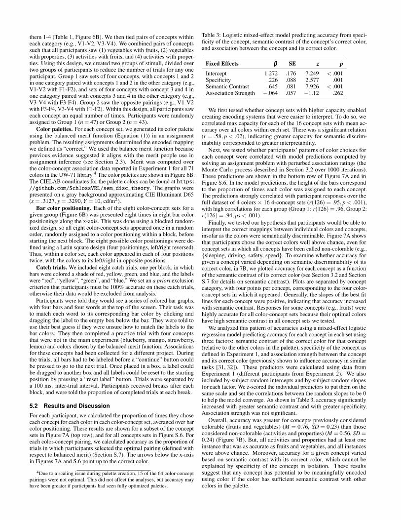
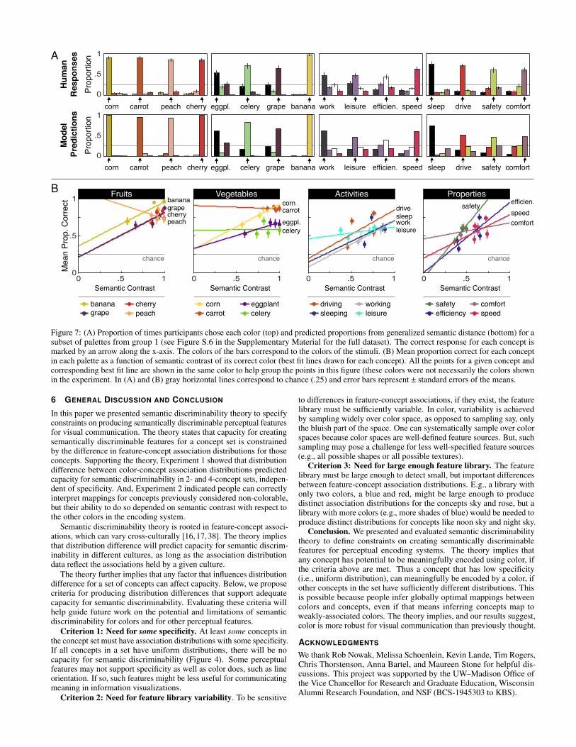
For each participant, we calculated the proportion of times they choseeach concept for each color in each color-concept set, averaged over barcolor positioning. These results are shown for a subset of the conceptsets in Figure 7A (top row), and for all concepts sets in Figure S.6. Foreach color-concept pairing, we calculated accuracy as the proportion oftrials in which participants selected the optimal pairing (defined withrespect to balanced merit) (Section S.7). The arrows below the x-axisin Figures 7A and S.6 point up to the correct color.
4Due to a scaling issue during palette creation, 15 of the 64 color-conceptpairings were not optimal. This did not affect the analyses, but accuracy mayhave been greater if participants had seen fully optimized palettes.
Table 3: Logistic mixed-effect model predicting accuracy from speci-ficity of the concept, semantic contrast of the concept’s correct color,and association between the concept and its correct color.
Fixed Effects βββ SE zzz ppp
Intercept 1.272 .176 7.249 < .001Specificity .226 .088 2.577 .001Semantic Contrast .645 .081 7.926 < .001Association Strength −.064 .057 −1.12 .262
We first tested whether concept sets with higher capacity enabledcreating encoding systems that were easier to interpret. To do so, wecorrelated max capacity for each of the 16 concept sets with mean ac-curacy over all colors within each set. There was a significant relation(r = .58, p < .02), indicating greater capacity for semantic discrim-inability corresponded to greater interpretability.
Next, we tested whether participants’ patterns of color choices foreach concept were correlated with model predictions computed bysolving an assignment problem with perturbed association ratings (theMonte Carlo process described in Section 3.2 over 1000 iterations).These predictions are shown in the bottom row of Figure 7A and inFigure S.6. In the model predictions, the height of the bars correspondto the proportion of times each color was assigned to each concept.The predictions strongly correlated with participant responses over thefull dataset of 4 colors × 16 4-concept sets (r(126) = .95, p < .001),with high correlations for each group (Group 1: r(126) = .96, Group 2:r(126) = .94, ps < .001).
Finally, we tested our hypothesis that participants would be able tointerpret the correct mappings between individual colors and concepts,insofar as the colors were semantically discriminable. Figure 7A showsthat participants chose the correct colors well above chance, even forconcept sets in which all concepts have been called non-colorable (e.g.,{sleeping, driving, safety, speed}. To examine whether accuracy forgiven a concept varied depending on semantic discriminability of itscorrect color, in 7B, we plotted accuracy for each concept as a functionof the semantic contrast of its correct color (see Section 3.2 and SectionS.7 for details on semantic contrast). Plots are separated by conceptcategory, with four points per concept, corresponding to the four color-concept sets in which it appeared. Generally, the slopes of the best fitlines for each concept were positive, indicating that accuracy increasedwith semantic contrast. Responses for some concepts (e.g., fruits) werehighly accurate for all color-concept sets because their optimal colorshave high semantic contrast in all concept sets we tested.
We analyzed this pattern of accuracies using a mixed-effect logisticregression model predicting accuracy for each concept in each set usingthree factors: semantic contrast of the correct color for that concept(relative to the other colors in the palette), specificity of the concept asdefined in Experiment 1, and association strength between the conceptand its correct color (previously shown to influence accuracy in similartasks [31, 32]). These predictors were calculated using data fromExperiment 1 (different participants from Experiment 2). We alsoincluded by-subject random intercepts and by-subject random slopesfor each factor. We z-scored the individual predictors to put them on thesame scale and set the correlations between the random slopes to be 0to help the model converge. As shown in Table 3, accuracy significantlyincreased with greater semantic contrast and with greater specificity.Association strength was not significant.
Overall, accuracy was greater for concepts previously consideredcolorable (fruits and vegetables) (M = 0.76, SD = 0.23) than thoseconsidered non-colorable (activities and properties) (M = 0.56, SD =0.24) (Figure 7B). But, all activities and properties had at least oneinstance that was as accurate as fruits and vegetables, and all instanceswere above chance. Moreover, accuracy for a given concept variedbased on semantic contrast with its correct color, which cannot beexplained by specificity of the concept in isolation. These resultssuggest that any concept has potential to be meaningfully encodedusing color if the color has sufficient semantic contrast with othercolors in the palette.
corn carrot peach cherry0
.5
1
Prop
ortio
n
eggpl. celery grape banana
eggpl. celery grape banana
sleep drive safety comfortwork leisure efficien. speed
work leisure efficien. speed sleep drive safety comfort0
.5
1
Prop
ortio
n
corn carrot peach cherry
Hum
an
Res
pons
esM
odel
Pre
dict
ions
A
0 .5 10
.5
1
Semantic Contrast
Mea
n Pr
op. C
orre
ct
drivingleisuresleepingworking comfort
efficiencysafety
speedcarrot celerycorn eggplantcherry
grape peach
bananagrape
peachcherry carrot
corn
eggpl.celery leisure
worksleepdrive speed
comfort
efficien.safety
B Fruits Vegetables Activities Properties
chance chance chance chance
0 .5 1Semantic Contrast
0 .5 1Semantic Contrast
0 .5 1Semantic Contrast
banana
Figure 7: (A) Proportion of times participants chose each color (top) and predicted proportions from generalized semantic distance (bottom) for asubset of palettes from group 1 (see Figure S.6 in the Supplementary Material for the full dataset). The correct response for each concept ismarked by an arrow along the x-axis. The colors of the bars correspond to the colors of the stimuli. (B) Mean proportion correct for each conceptin each palette as a function of semantic contrast of its correct color (best fit lines drawn for each concept). All the points for a given concept andcorresponding best fit line are shown in the same color to help group the points in this figure (these colors were not necessarily the colors shownin the experiment. In (A) and (B) gray horizontal lines correspond to chance (.25) and error bars represent ± standard errors of the means.
6 GENERAL DISCUSSION AND CONCLUSION
In this paper we presented semantic discriminability theory to specifyconstraints on producing semantically discriminable perceptual featuresfor visual communication. The theory states that capacity for creatingsemantically discriminable features for a concept set is constrainedby the difference in feature-concept association distributions for thoseconcepts. Supporting the theory, Experiment 1 showed that distributiondifference between color-concept association distributions predictedcapacity for semantic discriminability in 2- and 4-concept sets, indepen-dent of specificity. And, Experiment 2 indicated people can correctlyinterpret mappings for concepts previously considered non-colorable,but their ability to do so depended on semantic contrast with respect tothe other colors in the encoding system.
Semantic discriminability theory is rooted in feature-concept associ-ations, which can vary cross-culturally [16, 17, 38]. The theory impliesthat distribution difference will predict capacity for semantic discrim-inability in different cultures, as long as the association distributiondata reflect the associations held by a given culture.
The theory further implies that any factor that influences distributiondifference for a set of concepts can affect capacity. Below, we proposecriteria for producing distribution differences that support adequatecapacity for semantic discriminability. Evaluating these criteria willhelp guide future work on the potential and limitations of semanticdiscriminability for colors and for other perceptual features.
Criterion 1: Need for some specificity. At least some concepts inthe concept set must have association distributions with some specificity.If all concepts in a set have uniform distributions, there will be nocapacity for semantic discriminability (Figure 4). Some perceptualfeatures may not support specificity as well as color does, such as lineorientation. If so, such features might be less useful for communicatingmeaning in information visualizations.
Criterion 2: Need for feature library variability. To be sensitive
to differences in feature-concept associations, if they exist, the featurelibrary must be sufficiently variable. In color, variability is achievedby sampling widely over color space, as opposed to sampling say, onlythe bluish part of the space. One can systematically sample over colorspaces because color spaces are well-defined feature sources. But, suchsampling may pose a challenge for less well-specified feature sources(e.g., all possible shapes or all possible textures).
Criterion 3: Need for large enough feature library. The featurelibrary must be large enough to detect small, but important differencesbetween feature-concept association distributions. E.g., a library withonly two colors, a blue and red, might be large enough to producedistinct association distributions for the concepts sky and rose, but alibrary with more colors (e.g., more shades of blue) would be needed toproduce distinct distributions for concepts like noon sky and night sky.
Conclusion. We presented and evaluated semantic discriminabilitytheory to define constraints on creating semantically discriminablefeatures for perceptual encoding systems. The theory implies thatany concept has potential to be meaningfully encoded using color, ifthe criteria above are met. Thus a concept that has low specificity(i.e., uniform distribution), can meaningfully be encoded by a color, ifother concepts in the set have sufficiently different distributions. Thisis possible because people infer globally optimal mappings betweencolors and concepts, even if that means inferring concepts map toweakly-associated colors. The theory implies, and our results suggest,color is more robust for visual communication than previously thought.
ACKNOWLEDGMENTS
We thank Rob Nowak, Melissa Schoenlein, Kevin Lande, Tim Rogers,Chris Thorstenson, Anna Bartel, and Maureen Stone for helpful dis-cussions. This project was supported by the UW–Madison Office ofthe Vice Chancellor for Research and Graduate Education, WisconsinAlumni Research Foundation, and NSF (BCS-1945303 to KBS).
REFERENCES
[1] C. L. Anderson and A. C. Robinson. Affective congruence in visualizationdesign: Influences on reading categorical maps. IEEE Transactions onVisualization and Computer Graphics, 2021.
[2] L. Bartram, A. Patra, and M. Stone. Affective color in visualization. InProceedings of the 2017 CHI Conference on Human Factors in ComputingSystems, pages 1364–1374. ACM, 2017.
[3] B. Berlin and P. Kay. Basic Color Terms: Their Universality and Evolution.University of California Press, 1969.
[4] J. Bertin. Semiology of graphics: Diagrams, Networks, Maps. Universityof Wisconsin Press, Madison, 1983.
[5] R. J. Brockmann. The unbearable distraction of color. IEEE Transactionson Professional Communication, 34(3):153–159, 1991.
[6] R. Burkard, M. Dell’Amico, and S. Martello. Assignment Problems:revised reprint. SIAM, 2012.
[7] M. A. Changizi, Q. Zhang, and S. Shimojo. Bare skin, blood and theevolution of primate colour vision. Biology Letters, 2(2):217–221, 2006.
[8] B. R. Conway. Color vision, cones, and color-coding in the cortex. TheNeuroscientist, 15(3):274–290, 2009.
[9] J. R. De Leeuw. jspsych: A javascript library for creating behavioralexperiments in a web browser. Behavior Research Methods, 47(1):1–12,2015.
[10] A. J. Elliot, M. A. Maier, A. C. Moller, R. Friedman, and J. Meinhardt.Color and psychological functioning: the effect of red on performanceattainment. Journal of Experimental Psychology: General, 136(1):154,2007.
[11] H. Fang, S. Walton, E. Delahaye, J. Harris, D. Storchak, and M. Chen.Categorical colormap optimization with visualization case studies. IEEETransactions on Visualization and Computer Graphics, 23(1):871–880,2017.
[12] M. Hasantash, R. Lafer-Sousa, A. Afraz, and B. R. Conway. Paradoxicalimpact of memory on color appearance of faces. Nature Communications,10:1–10, 2019.
[13] C. Havasi, R. Speer, and J. Holmgren. Automated color selection usingsemantic knowledge. In 2010 AAAI Fall Symposium Series, 2010.
[14] N. Humphrey. The colour currency of nature. In T. Porter and B. Mikel-lides, editors, Colour for Architecture Today, pages 95–98. Taylor &Francis, 1976.
[15] A. Jahanian, S. Keshvari, S. Vishwanathan, and J. P. Allebach. Colors–messengers of concepts: Visual design mining for learning color semantics.ACM Transactions on Computer-Human Interaction, 24(1):2, 2017.
[16] D. Jonauskaite, A. M. Abdel-Khalek, A. Abu-Akel, A. S. Al-Rasheed,J.-P. Antonietti, A. G. Asgeirsson, K. A. Atitsogbe, M. Barma, D. Barratt,V. Bogushevskaya, et al. The sun is no fun without rain: Physical envi-ronments affect how we feel about yellow across 55 countries. Journal ofEnvironmental Psychology, 66:101350, 2019.
[17] D. Jonauskaite, J. Wicker, C. Mohr, N. Dael, J. Havelka, M. Papadatou-Pastou, M. Zhang, and D. Oberfeld. A machine learning approach toquantify the specificity of colour–emotion associations and their culturaldifferences. Royal Society Open Science, 6(9):190741, 2019.
[18] P. Kay, N. J. Smelser, P. B. Baltes, and B. Comrie. The Linguistics ofColor Terms. Citeseer, 2001.
[19] H. W. Kuhn. The hungarian method for the assignment problem. NavalResearch Logistics Quarterly, 2(1-2):83–97, 1955.
[20] S. Lin, J. Fortuna, C. Kulkarni, M. Stone, and J. Heer. Selectingsemantically-resonant colors for data visualization. In Computer GraphicsForum, volume 32, pages 401–410. Eurographics Conference on Visual-ization, 2013.
[21] A. Lindner, N. Bonnier, and S. Susstrunk. What is the color of chocolate?–extracting color values of semantic expressions. In Conference on Colourin Graphics, Imaging, and Vision, volume 2012, pages 355–361. Societyfor Imaging Science and Technology, 2012.
[22] A. Lindner, B. Z. Li, N. Bonnier, and S. Susstrunk. A large-scale multi-lingual color thesaurus. In Color and Imaging Conference, volume 2012,pages 30–35. Society for Imaging Science and Technology, 2012.
[23] J. Munkres. Algorithms for the assignment and transportation problems.Journal of the Society for Industrial and Applied Mathematics, 5(1):32–38,1957.
[24] F. Nielsen and R. Bhatia. Matrix Information Geometry. Springer BerlinHeidelberg, 2012.
[25] L.-C. Ou, M. R. Luo, A. Woodcock, and A. Wright. A study of colouremotion and colour preference. Part I: Colour emotions for single colours.
Color Research & Application, 29(3):232–240, 2004.[26] S. E. Palmer, K. B. Schloss, and J. Sammartino. Visual aesthetics and
human preference. Annual Review of Psychology, 64:77–107, 2013.[27] R. Rathore, Z. Leggon, L. Lessard, and K. B. Schloss. Estimating color-
concept associations from image statistics. IEEE Transactions on Visual-ization and Computer Graphics, 26(1):1226–1235, 2020.
[28] A. H. Robinson. The Look of Maps. University of Wisconsin Press,Madison, 1952.
[29] K. B. Schloss. A color inference framework. In . G. V. P. L. MacDonald,C. P. Biggam, editor, Progress in Colour Studies: Cognition, Language,and Beyond. John Benjamins, Amsterdam, 2018.
[30] K. B. Schloss, C. C. Gramazio, A. T. Silverman, M. L. Parker, and A. S.Wang. Mapping color to meaning in colormap data visualizations. IEEETransactions on Visualization and Computer Graphics, 25(1):810–819,2019.
[31] K. B. Schloss, Z. Leggon, and L. Lessard. Semantic discriminability forvisual communication. IEEE Transactions on Visualization and ComputerGraphics, 27(2):1022–1031, 2021.
[32] K. B. Schloss, L. Lessard, C. S. Walmsley, and K. Foley. Color inferencein visual communication: the meaning of colors in recycling. CognitiveResearch: Principles and Implications, 3(1):5, 2018.
[33] V. Setlur and M. C. Stone. A linguistic approach to categorical colorassignment for data visualization. IEEE Transactions on Visualization andComputer Graphics, 22(1):698–707, 2016.
[34] P. Shah and J. Hoeffner. Review of graph comprehension research: Im-plications for instruction. Educational Psychology Review, 14(1):47–69,2002.
[35] S. C. Sibrel, R. Rathore, L. Lessard, and K. B. Schloss. The relationbetween color and spatial structure for interpreting colormap data visual-izations. Journal of Vision, 20(12):7–7, 2020.
[36] M. Stone, D. A. Szafir, and V. Setlur. An engineering model for colordifference as a function of size. In Color and Imaging Conference, volume2014, pages 253–258. Society for Imaging Science and Technology, 2014.
[37] J. W. Tanaka and L. M. Presnell. Color diagnosticity in object recognition.Perception & Psychophysics, 61(6):1140–1153, 1999.
[38] D. S. Y. Tham, P. T. Sowden, A. Grandison, A. Franklin, A. K. W. Lee,M. Ng, J. Park, W. Pang, and J. Zhao. A systematic investigation of con-ceptual color associations. Journal of Experimental Psychology: General,149(7):1311–1332, 2020.
[39] C. A. Thorstenson, A. J. Elliot, A. D. Pazda, D. I. Perrett, and D. Xiao.Emotion-color associations in the context of the face. Emotion, 18(7):1032–1042, 2018.
[40] C. Witzel, H. Valkova, T. Hansen, and K. R. Gegenfurtner. Object knowl-edge modulates colour appearance. i-Perception, 2(1):13–49, 2011.
[41] G. Wyszecki and W. S. Stiles. Color Science. Wiley New York, 1982.
S SUPPLEMENTARY MATERIAL
S.1 UW-71 ColorsIn this study, we used a color library called the UW-71 (Figure S.1). Itis based on the UW-58 colors used in [27, 31], but extends to includelighter yellows and greens. The UW-58 colors includes 58 colors uni-formly sampled over CIELAB space (edge distance of ∆E = 25, rotatedof axis by 3 degrees to increase the number of colors, as describedin [27]). To obtain the UW-71, we sampled an additional plane ofcolors at lightness L = 88 with ∆E = 25. This provided 13 more colors,shown in the top plane of Figure S.1.
0
25
50
75
100UW-71 Colors
b
a80400-40-80
-80
800
Figure S.1: UW-71 colors plotted in CIELAB space.
S.2 Color-concept associationsFigure S.5A shows the mean color-concept association ratings col-lected in Experiment 1 (Section 4). Participants rated how much theyassociated each color from the UW-71 color library with each of 20concepts. In this figure, the order of the UW-71 colors along the x-axiswas obtained by sorting the colors according to CIE LCh hue anglewith achromatic colors being placed at the beginning of the list. FiguresS.5B shows a transformation of the data from Figure S.5A, turningmean ratings for each concept into a discrete probability distribution.This was done following the normalization process described in Section3.1. When we calculated entropy and (Generalized) Total Variation,we used data in this distribution form. Figure S.5C shows the samedata from Figure S.5B, sorted from high to low probability within eachconcept. In this sorted format, it is easier see how color-concept associ-ations vary in specificity for different concepts. We quantify specificityusing the entropy of the distribution, as described in Section 3.1.
S.3 Operationalizing specificity using entropyFigure S.2 shows the entropy for each concept, computed on the nor-malized color-concept association distributions (Figure S.5 B). Theconcepts are ordered from high specificity (low entropy) to low speci-ficity (high entropy), with example sorted association distributions atvarying levels of specificity. The top half of the concepts with highspecificity correspond to concepts that Lin et al. [20] called “colorable,”and the bottom half with low specificity correspond to concepts thatthey called “non-colorable”.
Concepts in Figure S.5C that have a steeper slope of descendingmean association probabilities have lower entropy and higher specificity.If one looks at the corresponding plots for each concept in Figure S.5Band entropy scores in Figure S.2, it can be seen that a concept canhave multiple peaks at different locations (such as eggplant) or a singlepeak (such as celery) and still have similar entropy (similar slopes ofordered mean association probabilities). This comparison highlightshow entropy is agnostic to any arbitrary ordering of colors and capturesthe ’peakiness’ or ’flatness’ of the distributions.
Hig
her S
peci
ficity
Low
er E
ntro
pyLo
wer
Spe
cific
ityH
ighe
r Ent
ropy
3.0 3.4 3.8 4.2Entropy
celerycelery
banana
peach
driving
safety
reliability
carrotcorn
bananaeggplant
applepeachgrape
mushroomcherry
sleepingspeedeatingdriving
workingcomfort
safetyefficiency
leisurereliability
Figure S.2: Entropy over color-concept association distributions (left)computed over the UW-71 color library, and examples of low- andhigh-entropy normed color-concept association distributions with colorsorted from high to low association (right). All of the concepts abovethe dashed line were considered colorable and the concepts below thedashed line were considered non-colorable in [20].
S.4 Operationalizing capacity
We considered four ways of operationalizing capacity for semanticdiscriminability: (1) Maximum semantic distance (computationallyidentical to maximum capacity), (2) Mean semantic distance, (3) Me-dian semantic distance, and (4) Proportion of semantic distances greaterthan some threshold (threshold capacity). For 2-concept sets, wecomputed all possible semantic distances for each possible color set(from the UW-71 library) within each concept set. We then comparedmean(∆S), median(∆S), and max capacity by computing the correla-tions between each pair of metrics for all possible feature sets withinall possible concept sets. Each correlation was strong (max and mean:r(188) = .86,p < .001; max and median: r(188) = .78, p < .001;mean and median: r(188) = .98, p < .001), so those three metrics weresimilar.
To assess threshold capacity, it is necessary to define a value of ∆Sto be used as the threshold. Figure S.3 shows the relation between thechoice of threshold value for threshold capacity and the correlationsbetween the resulting threshold capacity and TV (solid line) and meanentropy of the concept set (dashed line). The blue line shows that thestandard deviations of the ∆S values decrease as threshold increases.This decrease is expected because the average number of ∆S valuesgreater than some threshold will decrease the higher the threshold is.When the criterion for threshold is very high, only color sets withextremely high ∆S are above the threshold and thus there is very littlevariability in the values as is indicated by the blue curve. Thus, atvery high ∆S criteria, there is too little variability in capacity for itscorrelations with total variation and entropy to be interpreted. Moreover,prior work has shown that people’s accuracy at interpreting encodingmappings change very little for palettes with ∆S values higher than0.7 [31]. Due to these observations in addition to the lack of a principledway to pick a threshold for our data, we opted not to use thresholdcapacity.
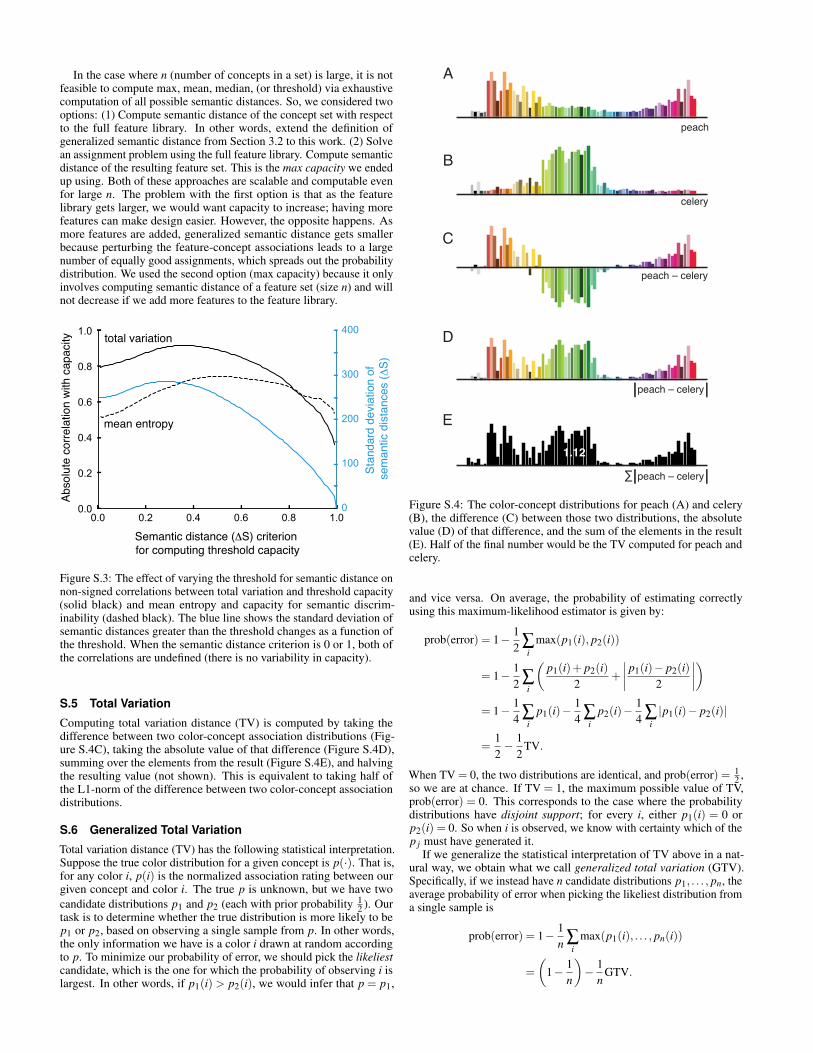
In the case where n (number of concepts in a set) is large, it is notfeasible to compute max, mean, median, (or threshold) via exhaustivecomputation of all possible semantic distances. So, we considered twooptions: (1) Compute semantic distance of the concept set with respectto the full feature library. In other words, extend the definition ofgeneralized semantic distance from Section 3.2 to this work. (2) Solvean assignment problem using the full feature library. Compute semanticdistance of the resulting feature set. This is the max capacity we endedup using. Both of these approaches are scalable and computable evenfor large n. The problem with the first option is that as the featurelibrary gets larger, we would want capacity to increase; having morefeatures can make design easier. However, the opposite happens. Asmore features are added, generalized semantic distance gets smallerbecause perturbing the feature-concept associations leads to a largenumber of equally good assignments, which spreads out the probabilitydistribution. We used the second option (max capacity) because it onlyinvolves computing semantic distance of a feature set (size n) and willnot decrease if we add more features to the feature library.
0.0 0.2 0.4 0.6 0.8 1.0
Semantic distance (ΔS) criterion for computing threshold capacity
0.0
0.2
0.4
0.6
0.8
1.0
Abso
lute
cor
rela
tion
with
cap
acity
0
100
200
300
400
Stan
dard
dev
iatio
n of
se
man
tic d
ista
nces
(ΔS)
total variation
mean entropy
Figure S.3: The effect of varying the threshold for semantic distance onnon-signed correlations between total variation and threshold capacity(solid black) and mean entropy and capacity for semantic discrim-inability (dashed black). The blue line shows the standard deviation ofsemantic distances greater than the threshold changes as a function ofthe threshold. When the semantic distance criterion is 0 or 1, both ofthe correlations are undefined (there is no variability in capacity).
S.5 Total Variation
Computing total variation distance (TV) is computed by taking thedifference between two color-concept association distributions (Fig-ure S.4C), taking the absolute value of that difference (Figure S.4D),summing over the elements from the result (Figure S.4E), and halvingthe resulting value (not shown). This is equivalent to taking half ofthe L1-norm of the difference between two color-concept associationdistributions.
S.6 Generalized Total Variation
Total variation distance (TV) has the following statistical interpretation.Suppose the true color distribution for a given concept is p(·). That is,for any color i, p(i) is the normalized association rating between ourgiven concept and color i. The true p is unknown, but we have twocandidate distributions p1 and p2 (each with prior probability 1
2 ). Ourtask is to determine whether the true distribution is more likely to bep1 or p2, based on observing a single sample from p. In other words,the only information we have is a color i drawn at random accordingto p. To minimize our probability of error, we should pick the likeliestcandidate, which is the one for which the probability of observing i islargest. In other words, if p1(i) > p2(i), we would infer that p = p1,
peach
celery
peach – celery
peach – celery
peach – celery�
A
B
C
D
E
1.12
Figure S.4: The color-concept distributions for peach (A) and celery(B), the difference (C) between those two distributions, the absolutevalue (D) of that difference, and the sum of the elements in the result(E). Half of the final number would be the TV computed for peach andcelery.
and vice versa. On average, the probability of estimating correctlyusing this maximum-likelihood estimator is given by:
prob(error) = 1− 12 ∑
imax(p1(i), p2(i))
= 1− 12 ∑
i
(p1(i)+ p2(i)
2+
∣∣∣∣ p1(i)− p2(i)2
∣∣∣∣)= 1− 1
4 ∑i
p1(i)−14 ∑
ip2(i)−
14 ∑
i|p1(i)− p2(i)|
=12− 1
2TV.
When TV = 0, the two distributions are identical, and prob(error) = 12 ,
so we are at chance. If TV = 1, the maximum possible value of TV,prob(error) = 0. This corresponds to the case where the probabilitydistributions have disjoint support; for every i, either p1(i) = 0 orp2(i) = 0. So when i is observed, we know with certainty which of thep j must have generated it.
If we generalize the statistical interpretation of TV above in a nat-ural way, we obtain what we call generalized total variation (GTV).Specifically, if we instead have n candidate distributions p1, . . . , pn, theaverage probability of error when picking the likeliest distribution froma single sample is
prob(error) = 1− 1n ∑
imax(p1(i), . . . , pn(i))
=
(1− 1
n
)− 1
nGTV.
In other words, we define GTV as:
GTV =−1+∑i
max(p1(i), . . . , pn(i))
When GTV = 0, again the distributions are all identical, and our prob-ability of error is 1− 1
n because we are at chance (we only have a1n chance of choosing correctly). When GTV = n− 1, its maximumpossible value, the n distributions have mutually disjoint support, so forevery i, at most one of the p j(i) is nonzero, which allows us to knowwith certainty which p j generated the sample, and the probability oferror is zero.
When n = 2, we get GTV = TV, which generalizes the standarddefinition of total variation distance. The trivial case n = 1 also makessense, because here GTV = 0 and the probability of error is also zero.
Although there are many notions of statistical distance for com-paring pairs of distributions, TV being among the simplest, there arevery few published techniques for comparing several distributions. Oneexample is the Frechet mean [24, p. 136]. To the best of our knowledge,our definition of generalized total variation is new.
S.7 Distinctions between Semantic Distance, SemanticContrast, and Accuracy in Experiment 2
Generalized semantic distance is an operationalization of semanticdiscriminability with respect to an entire color palette. It estimatesthe probability of inferring the most-likely unique mapping betweencolors and concepts, compared with all other possible mappings in anencoding system (Section 3.2).
For example, imagine a visualization depicting three concepts—apple, banana, and blueberry—with three colors—red, yellow, and blue.If we were to solve an assignment problem using the balanced meritfunction and raw association scores between all three colors and allthree concepts the most likely unique mapping would be: apple-red,banana-yellow, and blueberry-blue. If we repeatedly added randomnoise to the associations used as input and solved the assignment prob-lem (using a Monte Carlo process), we can compute the probabilityof this most likely assignment compared to all other assignments (e.g.,apple-yellow, banana-blue, blueberry-red, etc.).
Generalized semantic distance estimates people’s expectations aboutwhich colors map to which concepts, regardless of the “correct” assign-ment specified by the designer of an encoded system.
Semantic contrast is also an operationalization of semantic dis-tance, with respect to a single color relative to all other colors in apalette. It estimates the probability of inferring the optimal color-concept assignment for that color, where optimal is determined by anassignment problem using the balanced merit function. In the apple,banana, blueberry example above, the semantic contrast for, say, applewould be the proportion of times red was assigned to apple, comparedto all other concepts.
Like semantic distance, semantic contrast estimates which colormaps to which concept, regardless of the “correct” assignment specifiedby the designer of an encoding system.
Accuracy is the degree to which people’s interpretations of an cod-ing system of a visualization match the encoded mapping—the “correct”assignment between colors and concepts specified by the designer. Insome cases, the encoded mapping is explicitly specified by legends,labels, or other verbal descriptions, but encoded mappings can stillexist in the absence of such explicit specifications.
In Experiment 2 of the present study, we (designers) specified that theencoded mapping was the optimal mapping, generated by an assignmentproblem using the balanced merit function. Thus, accuracy for a givenconcept in a given concept set was the proportion of times participantschose the optimal color for that concept. We chose this definition ofaccuracy because previous work suggested assignments according tothe balanced merit function match people’s expectations (or inferredmappings). By matching people’s expectations, these palettes shouldhelp people be as accurate as possible. We aimed to create conditions inwhich participants could be as accurate as possible to test the hypothesisthat encoded mappings exist in which people can correctly interpretmappings for “non-colorable” concepts.
The conditions of Experiment 2 present a special case in whichsemantic contrast can be thought of as a model for accuracy. Thisis because both semantic contrast and accuracy are defined with re-spect to assignments using the balanced merit function. However, thiscorrespondence between accuracy and semantic contrast is not neces-sary. If the encoded mapping is defined in a different way that did notalign with the optimal assignment (e.g., a default palette order fromstandard software), then semantic contrast would no longer estimateaccuracy. For example, one could define the encoded mapping in theearlier example as follows: apple-yellow, banana-blue, blueberry-red.In this case, the semantic contrasts remain unchanged however people’saccuracies would be close to 0 for all colors (in the absence of a legend)because the encoded mapping heavily conflicts with people’s inferredmappings. Thus, semantic contrast is always an operationalization ofsemantic discriminability, but not necessarily an operationalization ofinterpretability.
If one wanted a general operationalization of interpretability, theycould adapt the method used to compute semantic contrast so thatinstead of estimating the probability of the optimal solution, it esti-mates the probability of the correct solution, according to the encodedmapping in an encoding system.
Additionally, if it were the case that there was a way of definingmerit scores used in the assignment problem that estimated people’sinferred mappings better than the balanced merit function, then ourmetrics including generalized semantic distance and semantic contrastcould be defined with respect to this merit function to better capturehuman behavior.
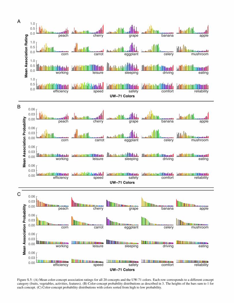
efficiency speed safety comfort reliability
working leisure sleeping driving eating
corn carrot eggplant celery mushroom
peach cherry grape banana apple0.000.030.06
0.000.030.06
0.000.030.06
0.000.030.06
UW−71 Colors
Mea
n A
ssoc
iatio
n Pr
obab
ility
efficiency speed safety comfort reliability
working leisure sleeping driving eating
corn carrot eggplant celery mushroom
peach cherry grape banana apple0.000.030.06
0.000.030.06
0.000.030.06
0.000.030.06
UW−71 Colors
Mea
n A
ssoc
iatio
n Pr
obab
ility
efficiency speed safety comfort reliability
working leisure sleeping driving eating
corn carrot eggplant celery mushroom
peach cherry grape banana apple0.00.51.0
0.00.51.0
0.00.51.0
0.00.51.0
UW−71 Colors
Mea
n A
ssoc
iatio
n R
atin
gA
B
C
Figure S.5: (A) Mean color-concept association ratings for all 20 concepts and the UW-71 colors. Each row corresponds to a different conceptcategory (fruits, vegetables, activities, features). (B) Color-concept probability distributions as described in 3. The heights of the bars sum to 1 foreach concept. (C) Color-concept probability distributions with colors sorted from high to low probability.
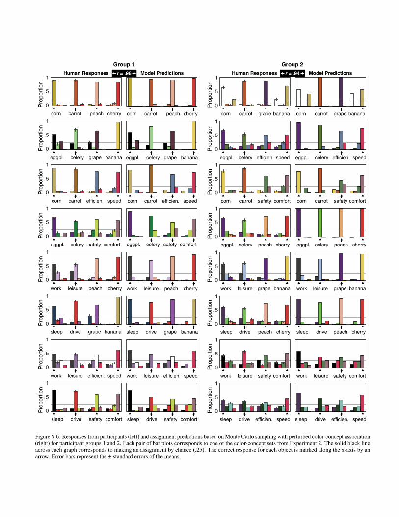
corn carrot grape banana
sleep drive peach cherry
work leisure safety comfort
eggpl. celery efficien. speed
work leisure grape banana
eggpl. celery peach cherry
corn carrot safety comfort
sleep drive efficien. speed
corn carrot peach cherry
sleep drive grape banana
work leisure efficien. speed
eggpl. celery safety comfort
work leisure peach cherry
eggpl. celery grape banana
corn carrot efficien. speed
sleep drive safety comfort
0
.5
1
Prop
ortio
n
0
.5
1
Prop
ortio
n
0
.5
1
Prop
ortio
n
0
.5
1
Prop
ortio
n
0
.5
1
Prop
ortio
n
0
.5
1
Prop
ortio
n
0
.5
1
Prop
ortio
n
0
.5
1
Prop
ortio
n
0
.5
1
Prop
ortio
n
0
.5
1
Prop
ortio
n
0
.5
1
Prop
ortio
n
0
.5
1
Prop
ortio
n
0
.5
1Pr
opor
tion
0
.5
1
Prop
ortio
n
0
.5
1
Prop
ortio
n
0
.5
1
Prop
ortio
n
Group 1Human Responses Model Predictionsr = .96 Human Responses Model Predictionsr = .94
Group 2
Figure S.6: Responses from participants (left) and assignment predictions based on Monte Carlo sampling with perturbed color-concept association(right) for participant groups 1 and 2. Each pair of bar plots corresponds to one of the color-concept sets from Experiment 2. The solid black lineacross each graph corresponds to making an assignment by chance (.25). The correct response for each object is marked along the x-axis by anarrow. Error bars represent the ± standard errors of the means.
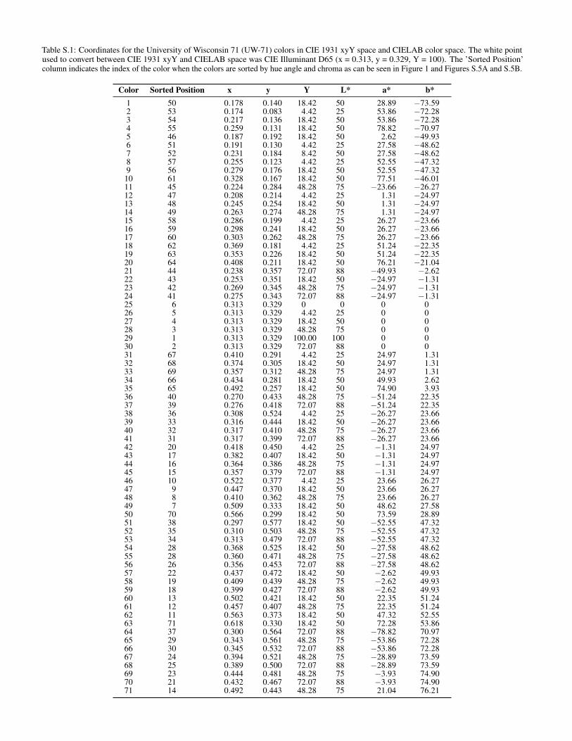
Table S.1: Coordinates for the University of Wisconsin 71 (UW-71) colors in CIE 1931 xyY space and CIELAB color space. The white pointused to convert between CIE 1931 xyY and CIELAB space was CIE Illuminant D65 (x = 0.313, y = 0.329, Y = 100). The ’Sorted Position’column indicates the index of the color when the colors are sorted by hue angle and chroma as can be seen in Figure 1 and Figures S.5A and S.5B.
Color Sorted Position x y Y L* a* b*1 50 0.178 0.140 18.42 50 28.89 −73.592 53 0.174 0.083 4.42 25 53.86 −72.283 54 0.217 0.136 18.42 50 53.86 −72.284 55 0.259 0.131 18.42 50 78.82 −70.975 46 0.187 0.192 18.42 50 2.62 −49.936 51 0.191 0.130 4.42 25 27.58 −48.627 52 0.231 0.184 8.42 50 27.58 −48.628 57 0.255 0.123 4.42 25 52.55 −47.329 56 0.279 0.176 18.42 50 52.55 −47.32
10 61 0.328 0.167 18.42 50 77.51 −46.0111 45 0.224 0.284 48.28 75 −23.66 −26.2712 47 0.208 0.214 4.42 25 1.31 −24.9713 48 0.245 0.254 18.42 50 1.31 −24.9714 49 0.263 0.274 48.28 75 1.31 −24.9715 58 0.286 0.199 4.42 25 26.27 −23.6616 59 0.298 0.241 18.42 50 26.27 −23.6617 60 0.303 0.262 48.28 75 26.27 −23.6618 62 0.369 0.181 4.42 25 51.24 −22.3519 63 0.353 0.226 18.42 50 51.24 −22.3520 64 0.408 0.211 18.42 50 76.21 −21.0421 44 0.238 0.357 72.07 88 −49.93 −2.6222 43 0.253 0.351 18.42 50 −24.97 −1.3123 42 0.269 0.345 48.28 75 −24.97 −1.3124 41 0.275 0.343 72.07 88 −24.97 −1.3125 6 0.313 0.329 0 0 0 026 5 0.313 0.329 4.42 25 0 027 4 0.313 0.329 18.42 50 0 028 3 0.313 0.329 48.28 75 0 029 1 0.313 0.329 100.00 100 0 030 2 0.313 0.329 72.07 88 0 031 67 0.410 0.291 4.42 25 24.97 1.3132 68 0.374 0.305 18.42 50 24.97 1.3133 69 0.357 0.312 48.28 75 24.97 1.3134 66 0.434 0.281 18.42 50 49.93 2.6235 65 0.492 0.257 18.42 50 74.90 3.9336 40 0.270 0.433 48.28 75 −51.24 22.3537 39 0.276 0.418 72.07 88 −51.24 22.3538 36 0.308 0.524 4.42 25 −26.27 23.6639 33 0.316 0.444 18.42 50 −26.27 23.6640 32 0.317 0.410 48.28 75 −26.27 23.6641 31 0.317 0.399 72.07 88 −26.27 23.6642 20 0.418 0.450 4.42 25 −1.31 24.9743 17 0.382 0.407 18.42 50 −1.31 24.9744 16 0.364 0.386 48.28 75 −1.31 24.9745 15 0.357 0.379 72.07 88 −1.31 24.9746 10 0.522 0.377 4.42 25 23.66 26.2747 9 0.447 0.370 18.42 50 23.66 26.2748 8 0.410 0.362 48.28 75 23.66 26.2749 7 0.509 0.333 18.42 50 48.62 27.5850 70 0.566 0.299 18.42 50 73.59 28.8951 38 0.297 0.577 18.42 50 −52.55 47.3252 35 0.310 0.503 48.28 75 −52.55 47.3253 34 0.313 0.479 72.07 88 −52.55 47.3254 28 0.368 0.525 18.42 50 −27.58 48.6255 28 0.360 0.471 48.28 75 −27.58 48.6256 26 0.356 0.453 72.07 88 −27.58 48.6257 22 0.437 0.472 18.42 50 −2.62 49.9358 19 0.409 0.439 48.28 75 −2.62 49.9359 18 0.399 0.427 72.07 88 −2.62 49.9360 13 0.502 0.421 18.42 50 22.35 51.2461 12 0.457 0.407 48.28 75 22.35 51.2462 11 0.563 0.373 18.42 50 47.32 52.5563 71 0.618 0.330 18.42 50 72.28 53.8664 37 0.300 0.564 72.07 88 −78.82 70.9765 29 0.343 0.561 48.28 75 −53.86 72.2866 30 0.345 0.532 72.07 88 −53.86 72.2867 24 0.394 0.521 48.28 75 −28.89 73.5968 25 0.389 0.500 72.07 88 −28.89 73.5969 23 0.444 0.481 48.28 75 −3.93 74.9070 21 0.432 0.467 72.07 88 −3.93 74.9071 14 0.492 0.443 48.28 75 21.04 76.21

![CDM [1ex]Context-Free Grammars](https://static.fdocument.org/doc/165x107/6267462bca88a44c0b14cdb5/cdm-1excontext-free-grammars.jpg)


![FLAC [1ex]Context-Sensitive Grammarsflac/pdf/lect-20.pdf · FLAC Context-Sensitive Grammars Klaus Sutner Carnegie Mellon Universality Fall 2017](https://static.fdocument.org/doc/165x107/5af8735b7f8b9aff288bd145/flac-1excontext-sensitive-flacpdflect-20pdfflac-context-sensitive-grammars.jpg)