Contents Introduction - Purdue Universitypatel471/locepsilon.pdf2 TOMOYUKI ABE AND DEEPAM PATEL When...
24
ON A LOCALIZATION FORMULA OF EPSILON FACTORS VIA MICROLOCAL GEOMETRY TOMOYUKI ABE AND DEEPAM PATEL Abstract. Given a lisse l-adic sheaf G on a smooth proper variety X and a lisse sheaf F on an open dense U in X, Kato and Saito conjectured a localization formula for the global l-adic epsilon factor ε l (X, F⊗G) in terms of the global epsilon factor of F and a certain intersection number associated to det(G) and the Swan class of F . In this article, we prove an analog of this conjecture for global de Rham epsilon factors in the classical setting of DX-modules on smooth projective varieties over a field of characteristic zero. Contents 1. Introduction 1 2. Background 3 3. Comparison of traces for various pairings of Picard groupoids 11 4. Localization formula for holonomic D X -modules 20 References 24 1. Introduction Let X denote a smooth proper variety of dimension d over a finite field F of characteristic p, and let G be a smooth ´ etale Q l (resp. F l ) sheaf. Then, one has the usual global l-adic epsilon factor ε l (X, F ) := 2d Y q=0 det(-σ :H q c (U ¯ F , F )) (-1) q , where σ ∈ Gal( ¯ F /F ) is the geometric Frobenius. In this setting, Kato and Saito conjectured the following ‘localization’ formula for the epsilon factor of the tensor product: Conjecture. ([3], 4.3.11) Let F be a constructible sheaf on X , and G be a smooth sheaf on X . Then one has ε l (X, F⊗G )= ε l (X, F ) rk(G) ·hdet(G ), CC(F )i. Here r G denotes the rank of G , and h-, -i denotes a pairing defined using the class field theory which we do not recall here. T.A. is supported by Grant-in-Aid for Young Scientists (A) 16H05993. D.P. would like to acknowledge support from the National Science Foundation award DMS-1502296. 1
Transcript of Contents Introduction - Purdue Universitypatel471/locepsilon.pdf2 TOMOYUKI ABE AND DEEPAM PATEL When...
ON A LOCALIZATION FORMULA OF EPSILON FACTORS VIA
MICROLOCAL GEOMETRY
TOMOYUKI ABE AND DEEPAM PATEL
Abstract. Given a lisse l-adic sheaf G on a smooth proper variety X and a lisse sheaf F onan open dense U in X, Kato and Saito conjectured a localization formula for the global l-adicepsilon factor εl(X,F ⊗ G) in terms of the global epsilon factor of F and a certain intersectionnumber associated to det(G) and the Swan class of F . In this article, we prove an analog of thisconjecture for global de Rham epsilon factors in the classical setting of DX -modules on smoothprojective varieties over a field of characteristic zero.
Contents
1. Introduction 12. Background 33. Comparison of traces for various pairings of Picard groupoids 114. Localization formula for holonomic DX -modules 20References 24
1. Introduction
Let X denote a smooth proper variety of dimension d over a finite field F of characteristicp, and let G be a smooth etale Ql (resp. Fl) sheaf. Then, one has the usual global l-adic epsilonfactor
εl(X,F) :=2d∏q=0
det(−σ : Hqc(UF ,F))(−1)q ,
where σ ∈ Gal(F /F ) is the geometric Frobenius. In this setting, Kato and Saito conjecturedthe following ‘localization’ formula for the epsilon factor of the tensor product:
Conjecture. ([3], 4.3.11) Let F be a constructible sheaf on X, and G be a smooth sheaf on X.Then one has
εl(X,F ⊗ G) = εl(X,F)rk(G) · 〈det(G),CC(F)〉.Here rG denotes the rank of G, and 〈−,−〉 denotes a pairing defined using the class field theorywhich we do not recall here.
T.A. is supported by Grant-in-Aid for Young Scientists (A) 16H05993. D.P. would like to acknowledge supportfrom the National Science Foundation award DMS-1502296.
1
2 TOMOYUKI ABE AND DEEPAM PATEL
When X is a proper smooth variety over a field k of characteristic 0, the second authorconstructed the de Rham epsilon factor formalism in ([8]). More precisely, let K(DX) denotethe K-theory spectrum of coherent DX -modules, and K(T ∗X) denote the K-theory spectrum ofcoherent sheaves. Then he constructed a map of spectra
ε : K(DX)→ K(T ∗X).
At the level of Grothendieck groups, given a holonomic module F , [ε(F)] ∈ K0(T ∗X) is the class[grF (F)] where F is a good filtration of F . It is well-known that the class is independent of thechoice of good filtration. The composition of ε with pullback by certain twist of the zero-sectionfollowed by the push-forward RΓ: K(X)→ K(k) is homotopic to the de Rham cohomology mapRΓdR (cf. Lemma 2.7.4). In particular, passing to Grothendieck groups, we may proceed viaε in order to compute the Euler-Poincare characteristic. Moreover, an automorphism f of Fdetermines an element in π1K(DX) whose image under the morphism RΓdR gives an elementof π1K(k) ∼= k×. The latter is precisely the determinant of the induced automorphism on thede Rham cohomology of F . In ([8]), a ‘microlocalized’ version of ε was also constructed, whichallows one to pass to the K-theory of holonomic DX -modules and construct a morphism ofspectra
CC : Khol(DX)→ K(d)(X,−).
Here Khol(DX) is the K-theory spectrum of holonomic DX -modules, and K(d)(X,−) is part ofLevine’s homotopy coniveau tower. We do not recall the definition here, but only note thatπ0(K(d)(X,−)) = CH0(X) and, at the level of π0, CC associates to the class of a holonomicDX -modules to the zero cycle given by pulling back it’s characteristic cycle by the zero section.Our main result is the following analog of the Kato-Saito localization formula in the de Rhamand K-theoretic setting:
Theorem (cf. 4.1.1). Let d be the dimension of X. The following diagram commutes up tohomotopy:
KX(DX) ∧Khol(DX)⊗ //
for∇∧CC��
Khol(DX)
RΓdR
��K(X) ∧K(d)(X,−)
〈−,−〉K(d,−)
// K(k).
The pairing 〈−,−〉K(d,−) is an analog in our setting of the pairing appearing in the conjecture
above. The usual dictionary between connective spectra and Picard groupoids allows one to getformulas for determinants of endomorphisms, and, in particular, by taking π1 of the commutativediagram above we get an equality of actual numbers analogous that in the conjecture above.We refer the reader to Theorem 4.3.1 for a precise statement. We note that this particularconsequence can be shown with a much simpler argument as described in loc. cit.. On the otherhand, by the same method, we also obtain similar formulas in the setting of correspondences (andnot just endomorphisms). In particular, suppose we are given an automorphism ϕ of X. Thena correspondence of a DX -module F is an isomorphism F → ϕ∗F . Given a correspondence,it induces an automorphism on the cohomology RΓdR(X,F), and we may again consider thedeterminant of this automorphism. We also obtain a localization formula in this setting.
ON A LOCALIZATION FORMULA OF EPSILON FACTORS VIA MICROLOCAL GEOMETRY 3
We note that, after most of this paper is written, the original conjecture of Kato and Saitohas been proven, with some modification of the definition of characteristic cycles and followingrecent developments in ramification theory for l-adic sheaves, in ([11]). However, followingthe philosophy of Beilinson (cf. [1]), we believe that the K-theoretic method gives a differentperspective on localization formulas for epsilon factors. In principal, proving the formula at thelevel of K-theory spectra should also give formulas in higher K-theory. At the level of K0 (resp.K1) one gets formulas for the Euler characteristic (resp. determinants). It would be interestingto see the consequences at the level of K2 (or higher K-groups).
Let us explain the structure of the paper. The paper begins with collecting some materialsfrom K-theory used in this paper. In particular, we recall some basic properties of Levine’shomotopy coniveau tower. In §3, we define the pairing 〈−,−〉K(d,−), and prove a key vanishing
lemma 3.7.1. This allows us to compute the pairing in the setting of correspondences. Weformulate and prove the localization formula in the last section. The localization formula as anequality of values is especially easy to prove when we are given actual automorphism of modules.We conclude the paper by providing an elementary proof of this simple case.
2. Background
In this article, we shall make use of K-theory spectra and their associated Picard groupoids.However, our applications will mostly use these constructions in a formal manner. We brieflyrecall the required concepts and constructions for ease of exposition.
2.1. (Spectra) In the following, we fix a symmetric monoidal category of spectra and denoteit by S. For example, one could take for S Lurie’s (∞, 1)-category of spectra or the categoryof symmetric spectra. We shall only make use of this category in a formal manner. Moreover,our results on traces only depend on the associated homotopy category (which are all known tobe equivalent for the various models for spectra). Recall that S is a proper simiplicial modelcategory. In particular, one has functorial fibrant-cofibrant replacements. In the following, weshall assume all our spectra are fibrant-cofibrant. We shall denote by ∧ the monoidal structurein S.
The homotopy category of S is denoted by Ho(S). By definition, this is the localization of Swith respect to the weak equivalences. A weak equivalence of spectra P → Q can be inverted asa morphism in the homotopy category. However, in general such a morphism cannot be invertedas a morphism of spectra. To remedy this situation, one must use the more general notion ofa homotopy morphism of spectra. A homotopy morphism P → Q consists of a contractiblesimplicial set K and a genuine morphism of spectra f : K ∧ P → Q. We refer to K as the baseof the homotopy morphism, and by abuse of notation we shall denote the homotopy morphismsimply by f : P → Q. Given two homotopy morphisms f, g with bases Kf ,Kg, an identificationof f and g is a homotopy morphism h with base Kh together with morphisms Kf → Kh ← Kg
such that f, g are the respective pullbacks of h. One can define the composition of two homotopymorphisms f : P → Q and g : Q → R as the composition Kg ∧ Kf ∧ P → Kg ∧ Q → R. Ahomotopy morphism from a sphere spectrum to a given spectrum P will be referred to as ahomotopy point of P . If f and g are identified, then they induce the same maps on homotopygroups. A weak equivalence between fibrant-cofibrant spectra can be canonically inverted as ahomotopy morphism. We refer to ([8], 2.1) or ([1], 1.4(ii)) for the details. We note that in thefollowing the language of homotopy morphisms is not necessary, since, for our purposes, we could
4 TOMOYUKI ABE AND DEEPAM PATEL
work directly in the homotopy category. However, it is a convenient notion for constructions atthe level of actual spectra (rather than the homotopy category).
2.2. (K-theory Spectra) Let E be a small exact category. Then Quillen’s K-theory construc-tion gives a functor from the category of small exact categories to the category of spectra. IfF1 : E1 → E2 and F2 : E2 → E3 are exact functors, then one has K(F2) ◦ K(F1) = K(F2 ◦ F1).More generally, a natural isomorphism of functors induces a homotopy equivalence of the corre-sponding morphisms of K-theory spectra. By taking a large enough Grothendieck universe, wemay assume all our categories are small.
More generally, Waldhausen associates to any category with cofibrations and weak equiva-lences a corresponding K-theory spectrum. Furthermore, an exact functor between Waldhausencategories induces a morphism between the corresponding spectra. In this article, we shallmostly be interested in complicial bi-Waldhausen categories and complicial exact functors; werefer the reader to ([10]) for details. If E is an exact category, then Cb(E) is a complicial bi-Waldhausen category with weak equivalences. A fundamental result of Thomason–Trobaugh–Waldhausen–Gillet ([10]) shows that the inclusion of E into Cb(E) as degree zero morphismsinduces a canonical weak equivalence of spectra K(E) → K(Cb(E)). Here the right side is theWaldhausen K-theory spectrum associated to Cb(E). This allows us to canonically identify var-ious Quillen and Waldhausen K-theory spectra. In the following, we shall always assume all ourspectra to be fibrant-cofibrant. In particular, the machinery from the previous section will allowus to invert various weak equivalences canonically as homotopy morphisms.
Given a Waldhausen category A, we denote by Atri the associated homotopy category givenby inverting the weak equivalences; note that this is a triangulated category. If F : A → Bis a complicial exact functor between two complicial bi-Waldhausen categories such that theinduced map on homotopy categories is an equivalence of categories, then the induced map onK-theory spectra is a weak equivalence. We will often consider derived functors which are apriori only defined on Atri. Usually, these can be lifted to functors on certain full complicialbi-Waldhausen subcategories C ⊂ A such that the inclusion induces an equivalence on theassociated triangulated categories. Using the formalism of homotopy morphisms, we can lift thederived functor to a morphism of K-theory spectra. A typical application is the following: LetX be a proper scheme over k, and let K(X) be the K-theory spectrum of perfect complexes onX. Since X is proper, we can define RΓ : Db
perf(X)→ Dbperf(k). The above approach allows us to
lift this to a homotopy morphism RΓ : K(X)→ K(k), where K(X) is the K-theory spectrum ofthe category of perfect complexes on X and similarly for K(k). First, we may consider the (full)complicial bi-Waldhausen sub-category of flasque perfect complexes. On this subcategory, RΓ isrepresented by Γ. Furthermore, the properness assumption implies that Γ preserves perfectness.We refer to the article by Thomason–Trobaugh ([10]) for more details.
Remark 2.2.1. Let X be a smooth projective variety over a field k, and DX the sheaf ofdifferential operators on X. Let K(DX) denote the K-theory spectrum of complexes of coherent-DX -modules. Then, via the above procedure, the DX -module pushforward induces a homotopymorphism RΓdR : K(DX) → K(k). For example, one can take the usual locally free resolutionby the de-Rham complex and restrict to flasque complexes.
2.3. (Picard groupoids, determinants, and traces) We recall some basic facts about Picardgroupoids and determinants which will be useful in the following. We refer to the beautifularticle ([2]) for the basic theory of Picard groupoids and determinants.
ON A LOCALIZATION FORMULA OF EPSILON FACTORS VIA MICROLOCAL GEOMETRY 5
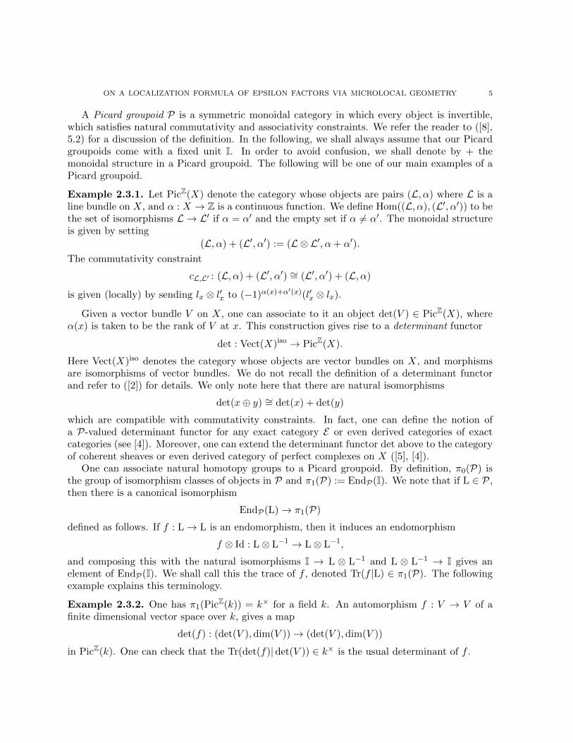
A Picard groupoid P is a symmetric monoidal category in which every object is invertible,which satisfies natural commutativity and associativity constraints. We refer the reader to ([8],5.2) for a discussion of the definition. In the following, we shall always assume that our Picardgroupoids come with a fixed unit I. In order to avoid confusion, we shall denote by + themonoidal structure in a Picard groupoid. The following will be one of our main examples of aPicard groupoid.
Example 2.3.1. Let PicZ(X) denote the category whose objects are pairs (L, α) where L is aline bundle on X, and α : X → Z is a continuous function. We define Hom((L, α), (L′, α′)) to bethe set of isomorphisms L → L′ if α = α′ and the empty set if α 6= α′. The monoidal structureis given by setting
(L, α) + (L′, α′) := (L ⊗ L′, α+ α′).
The commutativity constraint
cL,L′ : (L, α) + (L′, α′) ∼= (L′, α′) + (L, α)
is given (locally) by sending lx ⊗ l′x to (−1)α(x)+α′(x)(l′x ⊗ lx).
Given a vector bundle V on X, one can associate to it an object det(V ) ∈ PicZ(X), whereα(x) is taken to be the rank of V at x. This construction gives rise to a determinant functor
det : Vect(X)iso → PicZ(X).
Here Vect(X)iso denotes the category whose objects are vector bundles on X, and morphismsare isomorphisms of vector bundles. We do not recall the definition of a determinant functorand refer to ([2]) for details. We only note here that there are natural isomorphisms
det(x⊕ y) ∼= det(x) + det(y)
which are compatible with commutativity constraints. In fact, one can define the notion ofa P-valued determinant functor for any exact category E or even derived categories of exactcategories (see [4]). Moreover, one can extend the determinant functor det above to the categoryof coherent sheaves or even derived category of perfect complexes on X ([5], [4]).
One can associate natural homotopy groups to a Picard groupoid. By definition, π0(P) isthe group of isomorphism classes of objects in P and π1(P) := EndP(I). We note that if L ∈ P,then there is a canonical isomorphism
EndP(L)→ π1(P)
defined as follows. If f : L→ L is an endomorphism, then it induces an endomorphism
f ⊗ Id : L⊗ L−1 → L⊗ L−1,
and composing this with the natural isomorphisms I → L ⊗ L−1 and L ⊗ L−1 → I gives anelement of EndP(I). We shall call this the trace of f , denoted Tr(f |L) ∈ π1(P). The followingexample explains this terminology.
Example 2.3.2. One has π1(PicZ(k)) = k× for a field k. An automorphism f : V → V of afinite dimensional vector space over k, gives a map
det(f) : (det(V ), dim(V ))→ (det(V ), dim(V ))
in PicZ(k). One can check that the Tr(det(f)| det(V )) ∈ k× is the usual determinant of f .
6 TOMOYUKI ABE AND DEEPAM PATEL
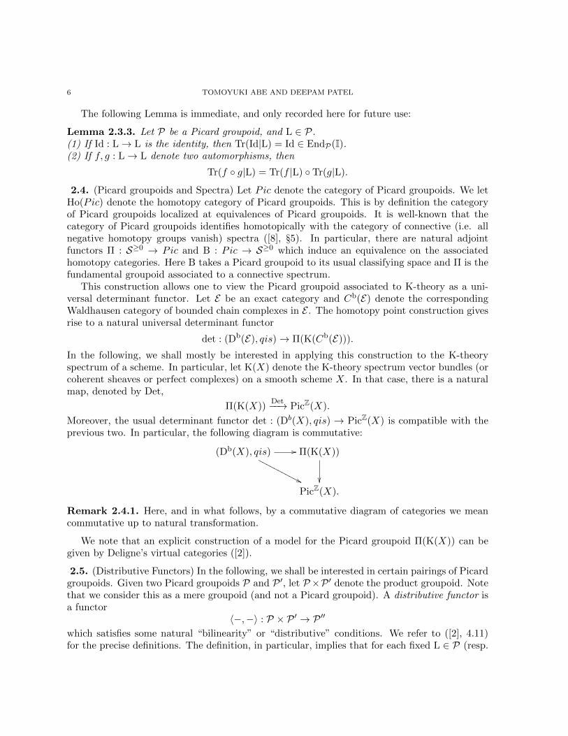
The following Lemma is immediate, and only recorded here for future use:
Lemma 2.3.3. Let P be a Picard groupoid, and L ∈ P.(1) If Id : L→ L is the identity, then Tr(Id|L) = Id ∈ EndP(I).(2) If f, g : L→ L denote two automorphisms, then
Tr(f ◦ g|L) = Tr(f |L) ◦ Tr(g|L).
2.4. (Picard groupoids and Spectra) Let Pic denote the category of Picard groupoids. We letHo(Pic) denote the homotopy category of Picard groupoids. This is by definition the categoryof Picard groupoids localized at equivalences of Picard groupoids. It is well-known that thecategory of Picard groupoids identifies homotopically with the category of connective (i.e. allnegative homotopy groups vanish) spectra ([8], §5). In particular, there are natural adjointfunctors Π : S≥0 → Pic and B : Pic → S≥0 which induce an equivalence on the associatedhomotopy categories. Here B takes a Picard groupoid to its usual classifying space and Π is thefundamental groupoid associated to a connective spectrum.
This construction allows one to view the Picard groupoid associated to K-theory as a uni-versal determinant functor. Let E be an exact category and Cb(E) denote the correspondingWaldhausen category of bounded chain complexes in E . The homotopy point construction givesrise to a natural universal determinant functor
det : (Db(E), qis)→ Π(K(Cb(E))).
In the following, we shall mostly be interested in applying this construction to the K-theoryspectrum of a scheme. In particular, let K(X) denote the K-theory spectrum vector bundles (orcoherent sheaves or perfect complexes) on a smooth scheme X. In that case, there is a naturalmap, denoted by Det,
Π(K(X))Det−−→ PicZ(X).
Moreover, the usual determinant functor det : (Db(X), qis) → PicZ(X) is compatible with theprevious two. In particular, the following diagram is commutative:
(Db(X), qis) //
''NNNNN
NNNNNN
Π(K(X))
��PicZ(X).
Remark 2.4.1. Here, and in what follows, by a commutative diagram of categories we meancommutative up to natural transformation.
We note that an explicit construction of a model for the Picard groupoid Π(K(X)) can begiven by Deligne’s virtual categories ([2]).
2.5. (Distributive Functors) In the following, we shall be interested in certain pairings of Picardgroupoids. Given two Picard groupoids P and P ′, let P×P ′ denote the product groupoid. Notethat we consider this as a mere groupoid (and not a Picard groupoid). A distributive functor isa functor
〈−,−〉 : P × P ′ → P ′′
which satisfies some natural “bilinearity” or “distributive” conditions. We refer to ([2], 4.11)for the precise definitions. The definition, in particular, implies that for each fixed L ∈ P (resp.
ON A LOCALIZATION FORMULA OF EPSILON FACTORS VIA MICROLOCAL GEOMETRY 7
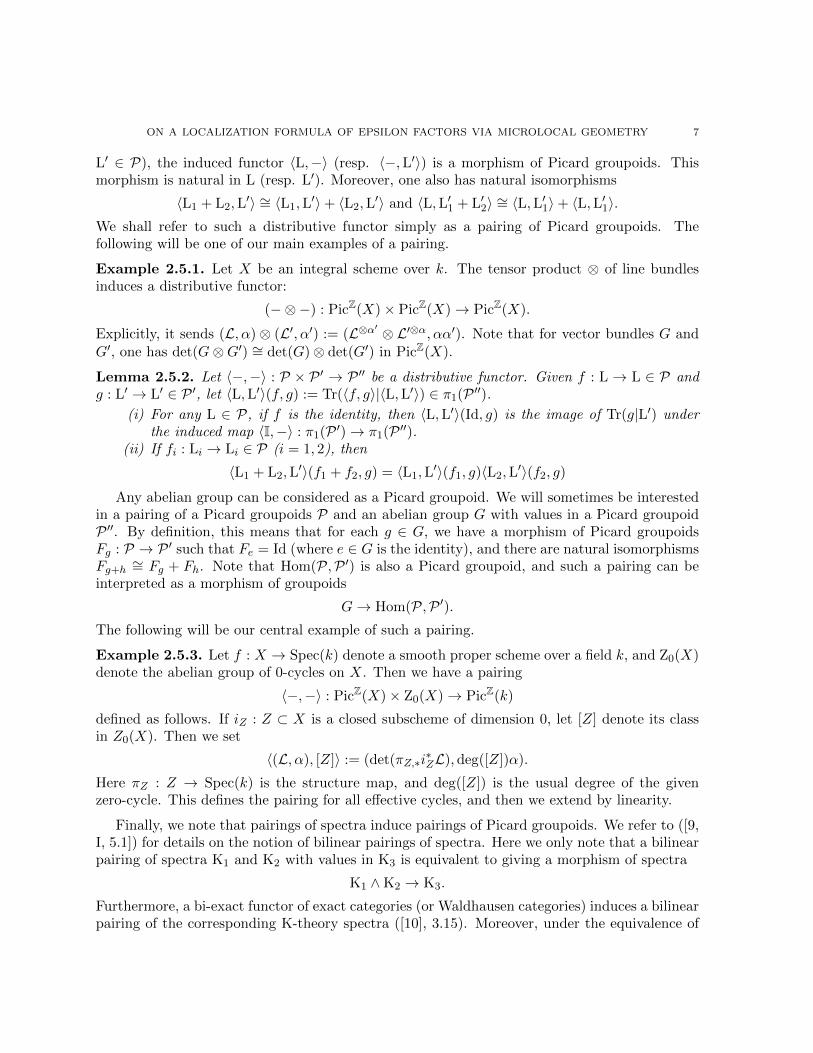
L′ ∈ P), the induced functor 〈L,−〉 (resp. 〈−,L′〉) is a morphism of Picard groupoids. Thismorphism is natural in L (resp. L′). Moreover, one also has natural isomorphisms
〈L1 + L2,L′〉 ∼= 〈L1,L
′〉+ 〈L2,L′〉 and 〈L,L′1 + L′2〉 ∼= 〈L,L′1〉+ 〈L,L′1〉.
We shall refer to such a distributive functor simply as a pairing of Picard groupoids. Thefollowing will be one of our main examples of a pairing.
Example 2.5.1. Let X be an integral scheme over k. The tensor product ⊗ of line bundlesinduces a distributive functor:
(−⊗−) : PicZ(X)× PicZ(X)→ PicZ(X).
Explicitly, it sends (L, α) ⊗ (L′, α′) := (L⊗α′ ⊗ L′⊗α, αα′). Note that for vector bundles G andG′, one has det(G⊗G′) ∼= det(G)⊗ det(G′) in PicZ(X).
Lemma 2.5.2. Let 〈−,−〉 : P × P ′ → P ′′ be a distributive functor. Given f : L → L ∈ P andg : L′ → L′ ∈ P ′, let 〈L,L′〉(f, g) := Tr(〈f, g〉|〈L,L′〉) ∈ π1(P ′′).
(i) For any L ∈ P, if f is the identity, then 〈L,L′〉(Id, g) is the image of Tr(g|L′) underthe induced map 〈I,−〉 : π1(P ′)→ π1(P ′′).
(ii) If fi : Li → Li ∈ P (i = 1, 2), then
〈L1 + L2,L′〉(f1 + f2, g) = 〈L1,L
′〉(f1, g)〈L2,L′〉(f2, g)
Any abelian group can be considered as a Picard groupoid. We will sometimes be interestedin a pairing of a Picard groupoids P and an abelian group G with values in a Picard groupoidP ′′. By definition, this means that for each g ∈ G, we have a morphism of Picard groupoidsFg : P → P ′ such that Fe = Id (where e ∈ G is the identity), and there are natural isomorphismsFg+h ∼= Fg + Fh. Note that Hom(P,P ′) is also a Picard groupoid, and such a pairing can beinterpreted as a morphism of groupoids
G→ Hom(P,P ′).The following will be our central example of such a pairing.
Example 2.5.3. Let f : X → Spec(k) denote a smooth proper scheme over a field k, and Z0(X)denote the abelian group of 0-cycles on X. Then we have a pairing
〈−,−〉 : PicZ(X)× Z0(X)→ PicZ(k)
defined as follows. If iZ : Z ⊂ X is a closed subscheme of dimension 0, let [Z] denote its classin Z0(X). Then we set
〈(L, α), [Z]〉 := (det(πZ,∗i∗ZL),deg([Z])α).
Here πZ : Z → Spec(k) is the structure map, and deg([Z]) is the usual degree of the givenzero-cycle. This defines the pairing for all effective cycles, and then we extend by linearity.
Finally, we note that pairings of spectra induce pairings of Picard groupoids. We refer to ([9,I, 5.1]) for details on the notion of bilinear pairings of spectra. Here we only note that a bilinearpairing of spectra K1 and K2 with values in K3 is equivalent to giving a morphism of spectra
K1 ∧K2 → K3.
Furthermore, a bi-exact functor of exact categories (or Waldhausen categories) induces a bilinearpairing of the corresponding K-theory spectra ([10], 3.15). Moreover, under the equivalence of
8 TOMOYUKI ABE AND DEEPAM PATEL
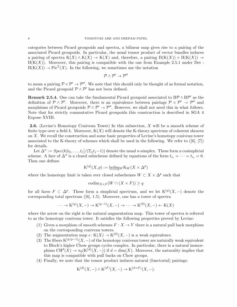
categories between Picard groupoids and spectra, a bilinear map gives rise to a pairing of theassociated Picard groupoids. In particular, the usual tensor product of vector bundles inducesa pairing of spectra K(X) ∧ K(X) → K(X) and, therefore, a pairing Π(K(X)) × Π(K(X)) →Π(K(X)). Moreover, this pairing is compatible with the one from Example 2.5.1 under Det :Π(K(X))→ PicZ(X). In the following, we sometimes use the notation
P ∧ P ′ → P ′′
to mean a pairing P×P ′ → P ′′. We note that this should only be thought of as formal notation,and the Picard groupoid P ∧ P ′ has not been defined.
Remark 2.5.4. One can take the fundamental Picard groupoid associated to BP ∧BP ′ as thedefinition of P ∧ P ′. Moreover, there is an equivalence between pairings P × P ′ → P ′′ andmorphisms of Picard groupoids P ∧ P ′ → P ′′. However, we shall not need this in what follows.Note that for strictly commutative Picard groupoids this construction is described in SGA 4Expose XVIII.
2.6. (Levine’s Homotopy Coniveau Tower) In this subsection, X will be a smooth scheme offinite type over a field k. Moreover, K(X) will denote the K-theory spectrum of coherent sheaveson X. We recall the construction and some basic properties of Levine’s homotopy coniveau towerassociated to the K-theory of schemes which shall be used in the following. We refer to ([6], [7])for details.
Let ∆n := Spec(k[t0, . . . , tr]/(Σjtj−1)) denote the usual n-simplex. These form a cosimplicialscheme. A face of ∆n is a closed subscheme defined by equations of the form ti1 = · · · = tis = 0.Then one defines
K(q)(X, p) := holim−−−→WKW (X ×∆p)
where the homotopy limit is taken over closed subschemes W ⊂ X ×∆p such that
codimX×F (W ∩ (X × F )) ≥ q
for all faces F ⊂ ∆p. These form a simplicial spectrum, and we let K(q)(X,−) denote thecorresponding total spectrum ([6], 1.5). Moreover, one has a tower of spectra
· · · → K(q)(X,−)→ K(q−1)(X,−)→ · · · → K(0)(X,−)← K(X)
where the arrow on the right is the natural augmentation map. This tower of spectra is referredto as the homotopy coniveau tower. It satisfies the following properties proved by Levine:
(1) Given a morphism of smooth schemes F : X → Y there is a natural pull back morphismon the corresponding coniveau towers.
(2) The augmentation map ε : K(X)→ K(0)(X,−) is a weak equivalence.
(3) The fibers K(p/p−1)(X,−) of the homotopy coniveau tower are naturally weak equivalentto Bloch’s higher Chow groups cycles complex. In particular, there is a natural isomor-phism CHd(X)→ π0(K(d)(X,−)) if d = dim(X). Moreover, the naturality implies thatthis map is compatible with pull backs on Chow groups.
(4) Finally, we note that the tensor product induces natural (functorial) pairings:
K(d)(X,−) ∧K(d′)(X,−)→ K(d+d′)(X,−).
ON A LOCALIZATION FORMULA OF EPSILON FACTORS VIA MICROLOCAL GEOMETRY 9
Remark 2.6.1. The existence of pairing as in (4) is a deep theorem and relies on Levine’smoving lemma for the homotopy coniveau tower. However, we shall only use the result in thecase where d′ = 0. In that case, K(0)(X,−) ∼= K(X), and the pairing is simply given by tensorproduct. In particular, no ‘moving’ is required.
2.7. (Microlocalization map of K-theory of DX -modules) In this paragraph, X will denote asmooth projective variety over a field k of characteristic zero. Below we recall the constructionof a microlocalization map for K-theory spectra of DX -modules. We refer to ([8]) for details.
Let K(DX) denote the K-theory spectrum of the abelian category of coherent DX -modules,and similarly let KS(DX) denote the K-theory spectrum of the abelian category of coherentDX -modules with singular support contained in S ⊂ T ∗X. Recall, any DX module M hasa good filtration F · such that the associated graded gives rise to a coherent OT ∗X -module.This construction gives rise to a well-defined (i.e. independent of the choice of filtration) mapK0(DX)→ K0(T ∗X). One has an analogous statement in the setting of supports. The followingtheorem extends this construction to the setting of higher K-theory.
Theorem 2.7.1. ([8]) Let X be as above. There is a natural microlocalization morphism ofK-theory spectra:
grS : KS(DX)→ KS(T ∗X).
Moreover, these are compatible with respect to the inclusions S ⊂ S′.
Let KF(DX) denote the K-theory spectrum of the exact category whose objects are pairs(M,F) where (M,F) is a coherent DX -module and F is a good filtration. We can similarlydefine KFS(DX). There is a natural map grF
S : KFS(DX) → KS(T ∗X) induced by sending apair (M,F) to grF (M). One also has a natural map ff : KFS(DX)→ KS(DX) given by simplyforgetting the filtration. By construction, grS ◦ ff is homotopic to grF
S .Let Khol(DX) denote the K-theory spectrum of the abelian category of holonomic DX -
modules. The preceding theorem immediately gives the following corollary by passing to homo-topy colimits.
Corollary 2.7.2. With notation as above, one has a morphism of spectra:
ε : Khol(DX)→ K(d)(T ∗X).
Proof. By definition, we may view the category of holonomic DX -modules as a direct limit of thecategories of the full sub-categories of DX -modules with singular support in a fixed codimensiond subset S ⊂ T ∗X. Since K-theory commutes with direct limits, we may write Khol(DX) as thecolimit of the corresponding spectra KS(DX). The result now follows from the previous theoremby taking limits. �
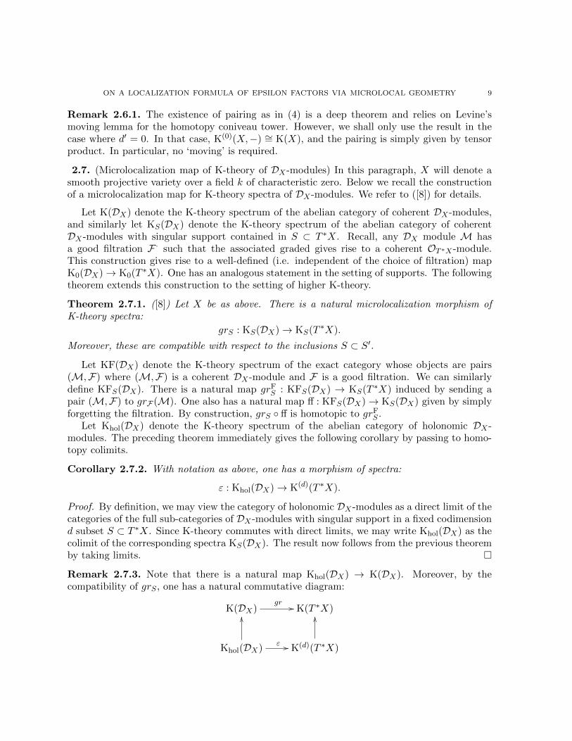
Remark 2.7.3. Note that there is a natural map Khol(DX) → K(DX). Moreover, by thecompatibility of grS , one has a natural commutative diagram:
K(DX)gr // K(T ∗X)
Khol(DX)ε //
OO
K(d)(T ∗X)
OO
10 TOMOYUKI ABE AND DEEPAM PATEL
Let f : X → Spec(k) denote the structure map, π : T ∗X → X the projection map, andσ : X → T ∗X the zero section. Then f and σ induce morphisms of K-theory spectra (2.2)
K(X)f∗−→ K(k) and K(T ∗X)
σ∗−→ K(X).
The canonical bundle ωX induces a natural morphism:
K(X)(−⊗ωX)−−−−−→ K(X).
We define the twisted pull-back σ+ as the composition:
K(T ∗X)σ∗−→ K(X)
(−⊗ωX)−−−−−→ K(X).
These give rise to a morphism f∗ ◦σ+ ◦ gr : K(DX)→ K(k). On the other hand, the DX -modulepushforward induces a morphism of K-theory spectra (2.2.1):
RΓdR : K(DX)→ K(k).
We have the following Lemma.
Lemma 2.7.4. The morphisms RΓdR and f∗ ◦ σ+ ◦ gr are homotopic.
Proof. For the first part, first note that the composition
K(X)→ K(DX)→ K(T ∗X)→ K(X)
is homotopic to the identity. Here the first map is the natural map induced by DX ⊗ (−), whichis a weak equivalence by a theorem of Quillen ([8]). Then one is reduced to showing that thecomposition
K(X)(−⊗ωX)−−−−−→ K(X)
f∗−→ K(k)
is homotopic to the composition
K(X)(DX⊗−)−−−−−→ K(DX)
RΓdR−−−→ K(k).
The latter follows from the fact that the corresponding functors are naturally isomorphic on thecorresponding derived categories. �
Remark 2.7.5. We think of RΓdR as the global de Rham epsilon factor. Recall, at the level ofDX -modules, up to a shift, the DX -module push-forward computes de Rham cohomology of thecorresponding DX -modules.
2.8. (Global epsilon factors and tensor products) We record an elementary lemma computingthe global epsilon factor of a tensor product.
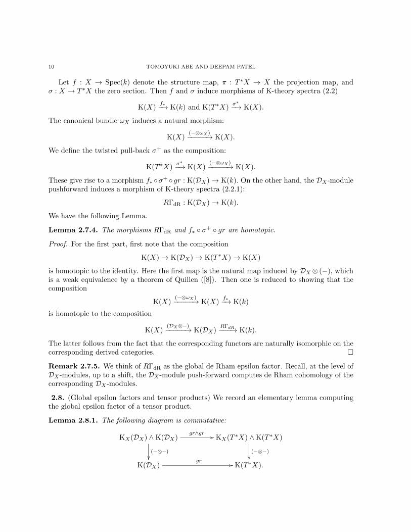
Lemma 2.8.1. The following diagram is commutative:
KX(DX) ∧K(DX)gr∧gr //
(−⊗−)��
KX(T ∗X) ∧K(T ∗X)
(−⊗−)��
K(DX)gr // K(T ∗X).
ON A LOCALIZATION FORMULA OF EPSILON FACTORS VIA MICROLOCAL GEOMETRY 11
Proof. The commutativity follows from the fact that gr commutes with tensor product if one ofthe sheaves is a bundle with connection. To be precise, we note that it is enough to show thatthe following diagram is homotopy commutative:
KX(DX) ∧K(X) //
(−⊗−)��
KX(T ∗X) ∧K(T ∗X)
(−⊗−)��
K(DX)gr // K(T ∗X)
Here the top horizontal is given by (gr∧gr)◦ (Id∧ (DX ⊗−). Since K(X)→ K(DX)→ K(T ∗X)is homotopic to π∗, the composition of the top horizontal and right vertical is homotopic toπ∗ ◦ (−⊗OX
−). On the other hand, there is a natural map KX(DX)→ KF(DX), and similarlyK(X)→ KF(DX), and the left vertical factors through KF(DX)∧KF(DX). The first map herejust gives a bundle with connection the trivial filtration. It’s now clear that the composition ofthis with lower horizontal with the left vertical is also homotopic to π∗ ◦ (−⊗OX
−). �
3. Comparison of traces for various pairings of Picard groupoids
In this subsection, we recall the construction of some pairings on K-theory spectra at thelevel of Levine’s homotopy coniveau tower, and make some computations of traces of tensorproducts in this setting.
3.1. (Pairings on K-theory with supports) Given a closed subset Z ⊂ X, there is a naturalpairing of K-theory spectra
K(X) ∧KZ(X)⊗−→ KZ(X)
induced by the tensor product ([10], 3.15). Since X is smooth, Quillen’s localization theorem im-plies that the natural map K(Z)→ KZ(X), induced by the push-forward, is a weak-equivalence.If iZ : Z ↪→ X is a reduced closed subscheme of dimension 0, and hence regular, then we mayidentify K(Z) with the K-theory spectrum of locally free sheaves. Moreover, one also has anatural pairing
K(X) ∧K(Z)→ K(Z) ∧K(Z)→ K(Z)
where the first map is induced by i∗Z ∧ Id. We record the following standard lemma for futureuse.
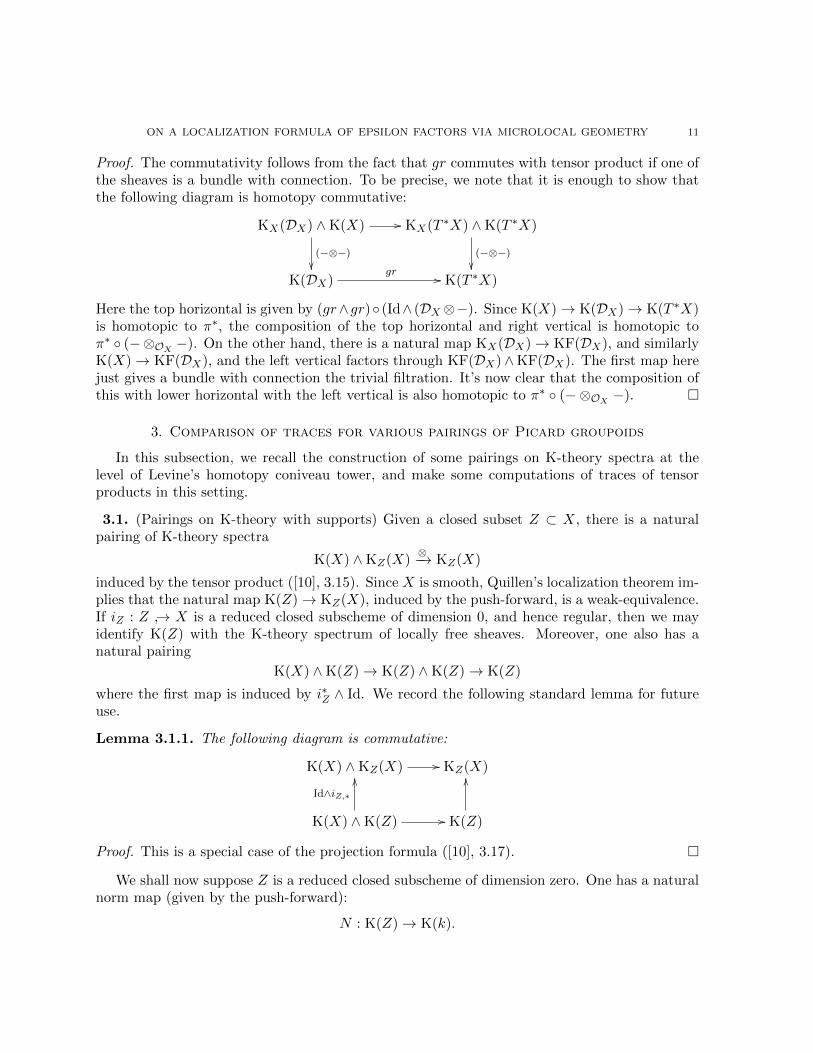
Lemma 3.1.1. The following diagram is commutative:
K(X) ∧KZ(X) // KZ(X)
K(X) ∧K(Z) //
Id∧iZ,∗
OO
K(Z)
OO
Proof. This is a special case of the projection formula ([10], 3.17). �
We shall now suppose Z is a reduced closed subscheme of dimension zero. One has a naturalnorm map (given by the push-forward):
N : K(Z)→ K(k).
12 TOMOYUKI ABE AND DEEPAM PATEL
Similarly, one has the usual push forward π∗ : KZ(X) → K(k). Composing the pairings abovewith these push-forward maps give rise to pairings:
〈−,−〉K : K(X) ∧KZ(X)→ K(k)
and
〈−,−〉K : K(X) ∧K(Z)→ K(k).
By the previous lemma these two pairings are identified via the natural weak equivalence iZ,∗ :K(Z) → KZ(X). Therefore, in the following we shall use the two interchangeably and use thesame notation to denote the two pairings.
Since the pairings above are compatible with respect to inclusions Z ′ ⊂ Z, we may pass tohomotopy limits and deduce a pairing:
〈−,−〉K(d) : K(X) ∧K(d)(X)→ K(k).
Note this pairing is simply the composition
K(X) ∧K(d)(X)(−⊗−)−−−−→ K(d)(X)
π∗−→ K(k).
Here we define π∗ as the one induced by taking homotopy limits of the maps π∗ : KZ(X)→ K(k).
Remark 3.1.2. We may also define π∗ by taking homotopy limits of the compositions KZ(X)→K(Z)
N−→ K(k). The two constructions are homotopic.
3.2. (Pairings on the homotopy coniveau tower) We now explain how the constructions of theprevious paragraph lift to Levine’s homotopy coniveau tower. Recall that we have a naturalaugmentation morphism
ε : K(d)(X)→ K(d)(X,−).
Moreover, there are natural pairings
K(r)(X,−) ∧K(s)(X,−)→ K(r+s)(X,−).
In particular, we may consider the composition
K(X) ∧K(d)(X)→ K(0)(X,−) ∧K(d)(X,−)→ K(d)(X,−).
Moreover, composing with π(d)∗ : K(d)(X,−) → K(0)(X,−) → K(X)
f∗−→ K(k) gives rise to apairing:
〈−,−〉K(d,−) : K(X) ∧K(d)(X,−)→ K(k).
Here we have inverted the augmentation map K(X) → K(0)(X,−). This pairing is compatiblewith the pairing constructed in the previous paragraph. Namely, we have the following lemma.
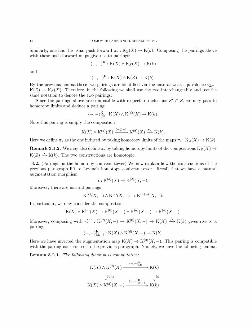
Lemma 3.2.1. The following diagram is commutative:
K(X) ∧K(d)(X)〈−,−〉K
(d) //
Id∧ε��
K(k)
Id
��K(X) ∧K(d)(X,−)
〈−,−〉K(d,−) // K(k)
ON A LOCALIZATION FORMULA OF EPSILON FACTORS VIA MICROLOCAL GEOMETRY 13
Proof. First, recall that the tensor product is compatible with the augmentation. Therefore, one
is reduced to showing that K(d)(X)ε−→ K(d)(X,−)
π(d)∗−−→ K(k) is homotopic to K(d)(X)
π∗−→ K(k).
The latter is evident from the construction of π(d)∗ . �
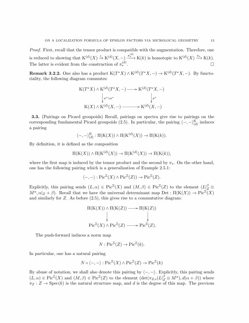
Remark 3.2.2. One also has a product K(T ∗X) ∧K(d)(T ∗X,−) → K(d)(T ∗X,−). By functo-riality, the following diagram commutes:
K(T ∗X) ∧K(d)(T ∗X,−) //
σ∗∧σ∗��
K(d)(T ∗X,−)
σ∗
��K(X) ∧K(d)(X,−) // K(d)(X,−)
3.3. (Pairings on Picard groupoids) Recall, pairings on spectra give rise to pairings on thecorresponding fundamental Picard groupoids (2.5). In particular, the pairing 〈−,−〉K(d) induces
a pairing
〈−,−〉Π(d) : Π(K(X)) ∧Π(K(d)(X))→ Π(K(k)).
By definition, it is defined as the composition
Π(K(X)) ∧Π(K(d)(X))→ Π(K(d)(X))→ Π(K(k)),
where the first map is induced by the tensor product and the second by π∗. On the other hand,one has the following pairing which is a generalization of Example 2.5.1:
〈−,−〉 : PicZ(X) ∧ PicZ(Z))→ PicZ(Z).
Explicitly, this pairing sends (L,α) ∈ PicZ(X) and (M,β) ∈ PicZ(Z) to the element (L|βZ ⊗Mα, α|Z + β). Recall that we have the universal determinant map Det : Π(K(X)) → PicZ(X)and similarly for Z. As before (2.5), this gives rise to a commutative diagram:
Π(K(X)) ∧Π(K(Z)) //
��
Π(K(Z))
��PicZ(X) ∧ PicZ(Z) // PicZ(Z).
The push-forward induces a norm map
N : PicZ(Z)→ PicZ(k).
In particular, one has a natural pairing
N ◦ 〈−,−〉 : PicZ(X) ∧ PicZ(Z)→ PicZ(k)
By abuse of notation, we shall also denote this pairing by 〈−,−〉. Explicitly, this pairing sends
(L,α) ∈ PicZ(X) and (M,β) ∈ PicZ(Z) to the element (det(πZ,∗(L|βZ ⊗Mα), d(α + β)) whereπZ : Z → Spec(k) is the natural structure map, and d is the degree of this map. The previous
14 TOMOYUKI ABE AND DEEPAM PATEL
remarks show that the following diagram commutes:
Π(K(X)) ∧Π(K(Z))〈−,−〉Π //
��
Π(K(k))
��PicZ(X) ∧ PicZ(Z)
〈−,−〉 // PicZ(k).
Remark 3.3.1. Recall that the map Det: Π(K(k)) → PicZ(k) is an isomorphism of Picardgroupoids. In the following, we shall make this identification in our resulting pairings.
3.4. (Picard groupoid pairings coming from coniveau tower) We now descend the pairings〈−,−〉K(d,−) to the level of Picard groupoids. In particular, taking fundamental groupoids gives
a pairing:
〈−,−〉Π(d,−) : Π(K(X)) ∧Π(K(d)(X,−))→ PicZ(k).
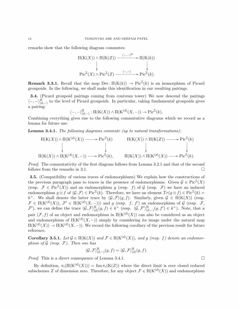
Combining everything gives rise to the following commutative diagrams which we record as alemma for future use:
Lemma 3.4.1. The following diagrams commute (up to natural transformations):
Π(K(X)) ∧Π(K(d)(X))
��
// PicZ(k)
��Π(K(X)) ∧Π(K(d)(X,−)) // PicZ(k),
Π(K(X)) ∧Π(K(Z))
��
// PicZ(k)
��Π(K(X)) ∧Π(K(d)(X)) // PicZ(k).
Proof. The commutativity of the first diagram follows from Lemma 3.2.1 and that of the secondfollows from the remarks in 3.1. �
3.5. (Compatibility of various traces of endomorphisms) We explain how the constructions ofthe previous paragraph pass to traces in the presence of endomorphisms. Given G ∈ PicZ(X)(resp. F ∈ PicZ(X)) and an endomorphism g (resp. f) of G (resp. F) we have an inducedendomorphism g⊗ f of 〈G,F〉 ∈ PicZ(k). Therefore, we have an element Tr(g⊗ f) ∈ PicZ(k) =k×. We shall denote the latter trace by 〈G,F〉(g, f). Similarly, given G ∈ Π(K(X)) (resp.
F ∈ Π(K(d)(X)), F ′ ∈ Π(K(d)(X,−))) and g (resp. f , f ′) an endomorphism of G (resp. F ,F ′), we can define the trace 〈G,F〉Π(d)(g, f) ∈ k× (resp. 〈G,F ′〉Π(d,−)(g, f
′) ∈ k×). Note, that a
pair (F , f) of an object and endomorphism in Π(K(d)(X)) can also be considered as an object
and endomorphism of Π(K(d)(X,−)) simply by considering its image under the natural map
Π(K(d)(X))→ Π(K(d)(X,−)). We record the following corollary of the previous result for futurereference.
Corollary 3.5.1. Let G ∈ Π(K(X)) and F ∈ Π(K(d)(X)), and g (resp. f) denote an endomor-phism of G (resp. F). Then one has
〈G,F〉Π(d,−)(g, f) = 〈G,F〉Π(d)(g, f).
Proof. This is a direct consequence of Lemma 3.4.1. �
By definition, πi(Π(K(d)(X))) = limπi(K(Z)) where the direct limit is over closed reduced
subschemes Z of dimension zero. Therefore, for any object F ∈ Π(K(d)(X)) and endomorphism
ON A LOCALIZATION FORMULA OF EPSILON FACTORS VIA MICROLOCAL GEOMETRY 15
f : F → F , we can choose a Z such that the pair (F , f) lifts to Π(K(Z)). In particular, there isa pair (FZ , fZ) consisting of an object and an endomorphism in Π(K(Z)), and an isomorphism
h of the image of this pair in Π(K(d)(X)) (under the natural map Π(K(Z))→ Π(K(d)(X))) withthe pair (F , f). In this setting, we have the following lemma;
Lemma 3.5.2. With notation as above, 〈G,F〉Π(d)(g, f) = 〈G,FZ〉Π(g, fZ). Moreover, we have
an equality 〈G,FZ〉Π(g, fZ) = 〈Det(G),Det(FZ)〉(g, fZ).
Proof. The first statement follows from the second commutative diagram in 3.4.1 after passingto Picard groupoids and traces. The second similarly follows from the remarks in 3.3. �
3.6. (Formula for traces of tensor products of endomorphisms) In this paragraph, we provean elementary formula for traces of tensor products of endomorphisms. In 3.9, shall prove asimilar formula in the more general the setting of correspondences. The formula presented inthis paragraph will be an easy corollary of that more general formula. However, we present thesimpler version here since the proof has some features of the more general situation and mightbe useful in understanding the more complicated version presented later.
Suppose we are given G ∈ Π(K(X)) (resp. F ∈ Π(K(d)(X))) with an endomorphism f : F →F and g : G → G as before. For any element of G ∈ Π(K(X)), we let rG (the rank of G) denoteits image in π0(PicZ(X)) = Z. In this setting, one has the following standard formula at thelevel of traces.
Proposition 3.6.1. With notation as above:
〈G,F〉Π(d)(g, f) = Tr(π∗(f)|π∗(F))rG 〈G,F〉Π(d)(g, Id).
Here, π∗(f) and π∗(F) are the images under the natural map Π(K(d)(X))π∗−→ PicZ(k).
Proof. By corollary 3.5.2, we are reduced to showing that
〈G,F〉(g, f) = Tr(det(πZ,∗(f))| det(πZ,∗(F)))rG 〈G,F〉(g, Id),
where G ∈ PicZ(X) and F ∈ PicZ(Z). Here iZ : Z ↪→ X is a closed integral subscheme ofdimension zero and πZ : Z → Spec(k) is the structure map. Since (by 2.3.3)
〈G,F〉(g, f) = 〈G,F〉(g, Id)〈G,F〉(Id, f),
we are reduced to showing that
〈G,F〉(Id, f) = Tr(det(πZ,∗(f)|det(πZ,∗(F)))rG .
We may further assume Z is irreducible. Then by definition (ignoring the grading)
〈G,F〉 = det(iZ,∗(G|Z ⊗F)) = det(iZ,∗(G|Z))rF ⊗ det(iZ,∗(F))rG .
The first equality here is consequence of the fact that iZ,∗ commutes with tensor products andsends locally free sheaves to locally free sheaves (since iZ is finite and flat). The second is theusual formula for determinant of a tensor product (i.e. the fact that det is a distributive functor).Moreover, we are computing the trace of the morphism induced by Id⊗ f on this object. Sincethe trace of the determinant of Id is one, we have
〈G,F〉(Id, f) = Tr(det(iZ,∗(f)|det(iZ,∗(F)))rG ,
which concludes the proof �
16 TOMOYUKI ABE AND DEEPAM PATEL
3.7. (A key vanishing Lemma) We would like a formula similar to that of the last paragraph for
〈G,F〉Π(d,−)(g, f) where F ∈ Π(K(d)(X)). If the pair (F , f) can be lifted to Π(K(d)(X)), then we
would get such a formula as a consequence of the previous proposition. Unfortunately, while wemay lift any such object F to Π(K(d)(X)), it is not always possible to lift the endomorphism f .However, we shall see that the desired formula (in the more general setting of correspondences)will be an easy consequence of the following lemma.
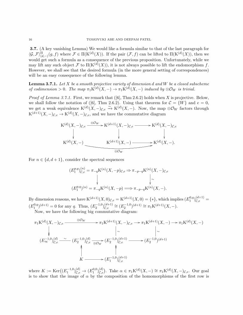
Lemma 3.7.1. Let X be a smooth projective variety of dimension d and W be a closed subschemeof codimension > 0. The map π1K(d)(X,−)→ π1K(d)(X,−) induced by ⊗OW is trivial.
Proof of Lemma 3.7.1. First, we remark that ([6], Thm 2.6.2) holds whenX is projective. Below,we shall follow the notation of ([6], Thm 2.6.2). Using that theorem for C = {W} and e = 0,
we get a weak equivalence K(d)(X,−)C,e∼−→ K(d)(X,−). Now, the map ⊗OW factors through
K(d+1)(X,−)C,e → K(d)(X,−)C,e, and we have the commutative diagram
K(d)(X,−)C,e⊗OW //
��
K(d+1)(X,−)C,e //
��
K(d)(X,−)C,e
��K(d)(X,−)
⊗OW
22K(d+1)(X,−) // K(d)(X,−).
For n ∈ {d, d+ 1}, consider the spectral sequences
(Ep,q1 )(n)C,e = π−qK
(n)(X,−p)C,e +3
��
π−p−qK(n)(X,−)C,e
∼��
(Ep,q1 )(n) = π−qK(n)(X,−p) +3 π−p−qK
(n)(X,−).
By dimension reasons, we have K(d+1)(X, 0)C,e = K(d+1)(X, 0) = {∗}, which implies (E0,q1 )
(d+1)C,e =
(E0,q1 )(d+1) = 0 for any q. Thus, (E−1,0
2 )(d+1)C,e
∼= (E−1,02 )(d+1) ∼= π1K(d+1)(X,−).
Now, we have the following big commutative diagram:
π1K(d)(X,−)C,e⊗OW //
����
π1K(d+1)(X,−)C,e
∼
// π1K(d+1)(X,−)
∼
// π1K(d)(X,−)
(E−1,0∞ )
(d)C,e
∼(E−1,0
2 )(d)C,e ⊗OW
// (E−1,02 )
(d+1)C,e
// (E−1,02 )(d+1)
K
OOOO
// (E−1,01 )
(d+1)C,e
OOOO
where K := Ker((E−1,0
1 )(d)C,e → (E0,0
1 )(d)C,e). Take α ∈ π1K(d)(X,−) ∼= π1K(d)(X,−)C,e. Our goal
is to show that the image of α by the composition of the homomorphisms of the first row is
ON A LOCALIZATION FORMULA OF EPSILON FACTORS VIA MICROLOCAL GEOMETRY 17
trivial. By the diagram above, there exists
α ∈ K ⊂ (E−1,01 )
(d)C,e = π0K(d)(X, 1)C,e
such that α ⊗ OW coincides with α ⊗ OW in π1K(d+1)(X,−)C,e. It suffices to show that the
image of α⊗OW in (E−1,02 )(d+1) is 0.
There exists a closed subscheme Z ⊂ X × ∆1 belonging to S(d)X,C,e(1) (in particular, dimen-
sion 1) such that α can be lifted to KZ(X, 1), which we denote by α′. We have α′ ⊗ OW ∈π0KZ∩pr−1(W )(X × ∆1) (where pr : X × ∆1 → X is the projection). Since Z ∈ S(d)
X,C,e(1), the
intersection Z ∩ pr−1(W ) is 0-dimensional. By definition of S(d)X,C,e(1), note that Z ∩ pr−1(W ) ⊂
X × (∆1 \ {0, 1}). The canonical coordinates of ∆2 is denoted by t1, t2. Take a closed point(w, s) ∈ X × (∆1 \ {0, 1}). Let
H(w,s) := {w} ×{t1 + st2 − s = 0
}⊂ X ×∆2,
namely the closed subscheme in {w}×∆2 which is the line connecting (s, 0) and (0, 1). We havethe morphism ρ(w,s) : H(w,s) → {(w, s)} ↪→ X ×∆1. Now, put
β :=⊕
(w,s)∈Z∩pr−1(W )
ρ∗(w,s)(α′ ⊗OW ) ∈ π0KH(X ×∆2) (H :=
⋃(w,s)∈Z∩pr−1(W )
H(w,s))
By construction, this will give a homotopy between α′ ⊗OW and 0. Indeed, let f1 : X ×∆1 ↪→X×∆2 be the map defined by t2 = 1, f3 by t1 = 0, f2 by t1 + t2 = 1 sending 0, 1 to (0, 1), (1, 0)respectively. The homotopy β defines
f∗1 (β) + f∗2 (β) ∼ f∗3 (β).
On the other hand, f∗1 (β) = α′ ⊗OW and f∗2 (β) = f∗3 (β), thus α′ ⊗OW is homotopic to 0. �
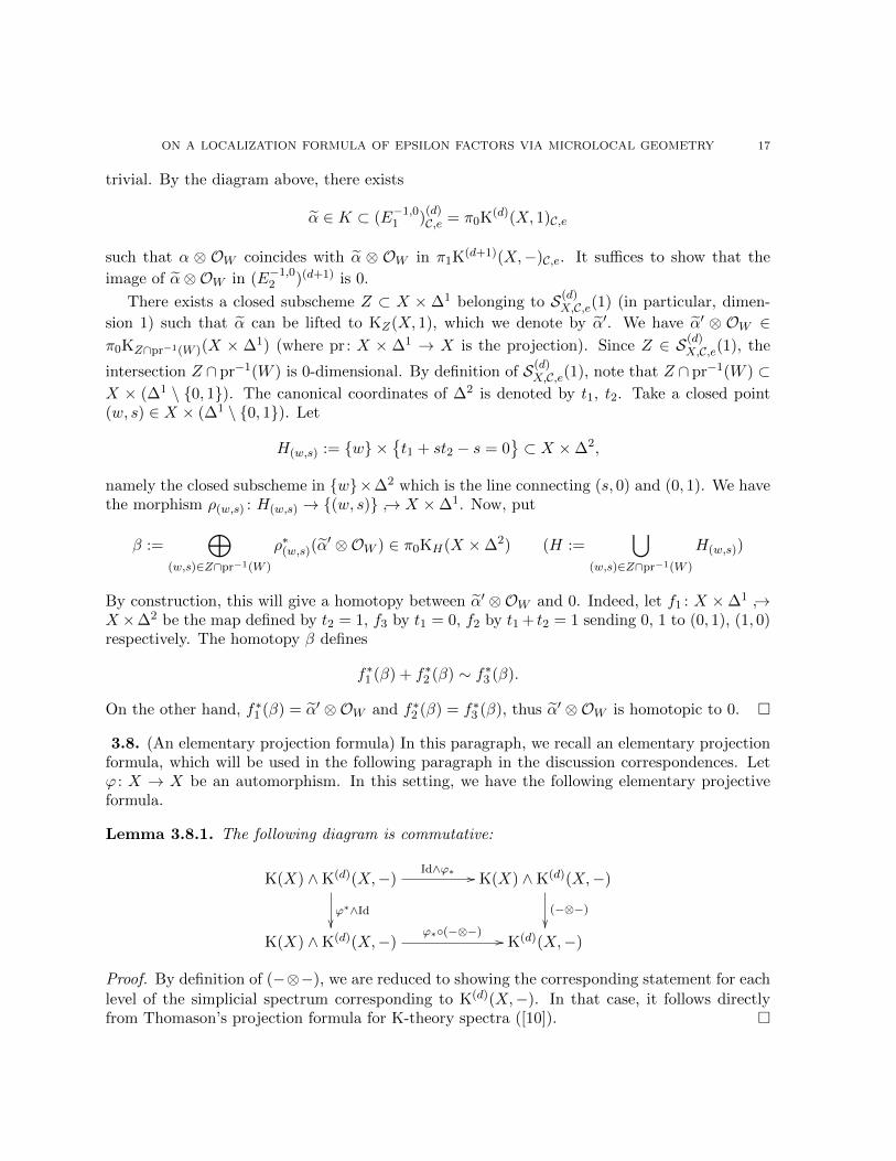
3.8. (An elementary projection formula) In this paragraph, we recall an elementary projectionformula, which will be used in the following paragraph in the discussion correspondences. Letϕ : X → X be an automorphism. In this setting, we have the following elementary projectiveformula.
Lemma 3.8.1. The following diagram is commutative:
K(X) ∧K(d)(X,−)Id∧ϕ∗ //
ϕ∗∧Id��
K(X) ∧K(d)(X,−)
(−⊗−)��
K(X) ∧K(d)(X,−)ϕ∗◦(−⊗−) // K(d)(X,−)
Proof. By definition of (−⊗−), we are reduced to showing the corresponding statement for each
level of the simplicial spectrum corresponding to K(d)(X,−). In that case, it follows directlyfrom Thomason’s projection formula for K-theory spectra ([10]). �
18 TOMOYUKI ABE AND DEEPAM PATEL
It follows that we have a commutative diagram at the level of Picard groupoids:
Π(K(X)) ∧Π(K(d)(X,−))Id∧ϕ∗ //
ϕ∗∧Id��
Π(K(X)) ∧Π(K(d)(X,−))
(−⊗−)��
Π(K(X)) ∧Π(K(d)(X,−))ϕ∗◦(−⊗−) // Π(K(d)(X,−))
In particular, for G ∈ Π(K(d)(X,−)) and F ∈ Π(K(d)(X,−)) we have natural isomorphisms
projG,F : ϕ∗(ϕ∗(G)⊗F)→ G ⊗ ϕ∗F .
3.9. (Formula for traces of tensor products of correspondences) We shall now prove a formulafor the traces of tensor products of correspondences. Let ϕ : X → X be an endomorphism. Thenone has an induced map ϕ∗ : K(d)(X,−)→ K(d)(X,−). Moreover, we also have the pushforwardmap
π(d)∗ : K(d)(X,−)→ K(k).
Note that π(d)∗ ◦ϕ∗ is homotopic to (π
(d)∗ ◦ϕ)∗ = π
(d)∗ . Below, we use the same notation to denote
the corresponding induced morphisms on the associated Picard groupoids.
Definition 3.9.1. Let F ∈ ΠK(d)(X,−). A correspondence ΦF on F is a morphism ΦF : F →ϕ∗F in ΠK(d)(X,−).
Let (F ,ΦF ) be an object in ΠK(d)(X,−) endowed with a correspondence. Then we havemorphisms
π(d)∗ (ΦF ) : π
(d)∗ (F)→ π
(d)∗ (ϕ∗F) ∼= π
(d)∗ (F)
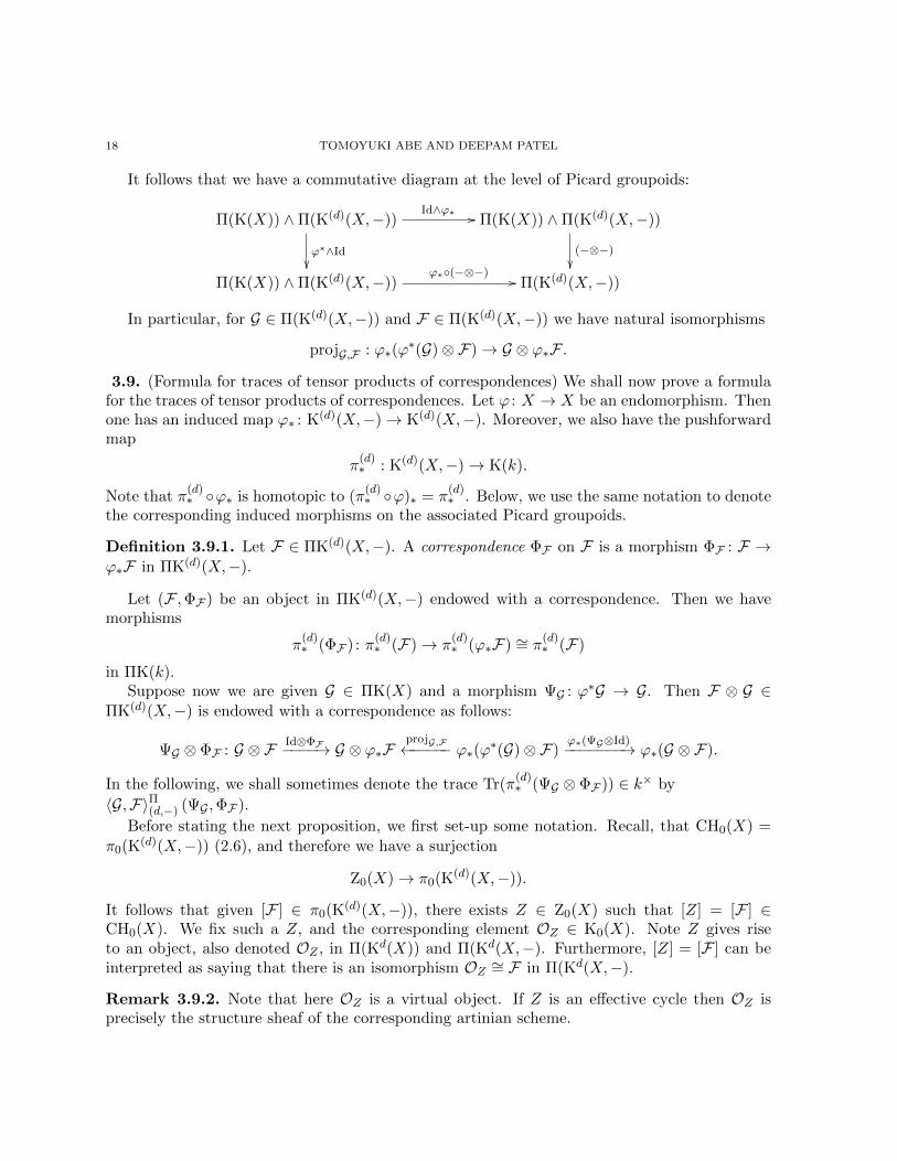
in ΠK(k).Suppose now we are given G ∈ ΠK(X) and a morphism ΨG : ϕ∗G → G. Then F ⊗ G ∈
ΠK(d)(X,−) is endowed with a correspondence as follows:
ΨG ⊗ ΦF : G ⊗ F Id⊗ΦF−−−−→ G ⊗ ϕ∗FprojG,F←−−−−− ϕ∗(ϕ∗(G)⊗F)
ϕ∗(ΨG⊗Id)−−−−−−−→ ϕ∗(G ⊗ F).
In the following, we shall sometimes denote the trace Tr(π(d)∗ (ΨG ⊗ ΦF )) ∈ k× by
〈G,F〉Π(d,−) (ΨG ,ΦF ).
Before stating the next proposition, we first set-up some notation. Recall, that CH0(X) =
π0(K(d)(X,−)) (2.6), and therefore we have a surjection
Z0(X)→ π0(K(d)(X,−)).
It follows that given [F ] ∈ π0(K(d)(X,−)), there exists Z ∈ Z0(X) such that [Z] = [F ] ∈CH0(X). We fix such a Z, and the corresponding element OZ ∈ K0(X). Note Z gives riseto an object, also denoted OZ , in Π(Kd(X)) and Π(Kd(X,−). Furthermore, [Z] = [F ] can beinterpreted as saying that there is an isomorphism OZ ∼= F in Π(Kd(X,−).
Remark 3.9.2. Note that here OZ is a virtual object. If Z is an effective cycle then OZ isprecisely the structure sheaf of the corresponding artinian scheme.
ON A LOCALIZATION FORMULA OF EPSILON FACTORS VIA MICROLOCAL GEOMETRY 19
Recall that for an object G ∈ Π(K(X)) we can consider its generic rank rG (i.e. the imageof G in π0(PicZ(X)) = Z), and that there is an object G0 ∈ Π(K(X)) of generic rank 0 suchthat G ∼= det(OrGX ) + G0 ∈ Π(K(X)). For the latter statement, note that by a Lemma ofSerre, any object [G] ∈ K0(X) can be written as [G0] + [OrGX ] ∈ K0(X). It follows that one hasan isomorphism between G and det(G0) + det(OrGX ) in Π(K(X)). In the following, we denotedet(OrGX ) simply by OrGX and det(G0) by G0. Note that OX comes equipped with a canonicalcorrespondence can : π∗OX → OX , and therefore OrGX also comes equipped with a canonicalcorrespondence (also denoted can). As a result, G0 = G + (OrGX )−1 also comes equipped with acorrespondence. We shall denote the it by ΨG0 .
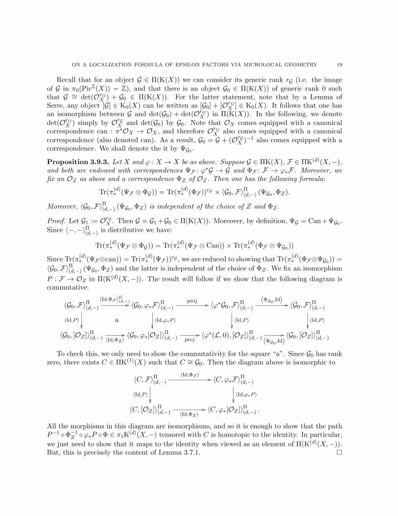
Proposition 3.9.3. Let X and ϕ : X → X be as above. Suppose G ∈ ΠK(X), F ∈ ΠK(d)(X,−),and both are endowed with correspondences ΨF : ϕ∗G → G and ΦF : F → ϕ∗F . Moreover, wefix an OZ as above and a correspondence ΦZ of OZ . Then one has the following formula:
Tr(π(d)∗ (ΨF ⊗ ΦG)) = Tr(π
(d)∗ (ΦF ))rG × 〈G0,F〉Π(d,−) (ΨG0 ,ΦZ).
Moreover, 〈G0,F〉Π(d,−) (ΨG0 ,ΦZ) is independent of the choice of Z and ΦZ .
Proof. Let G1 := OrGX . Then G = G1 +G0 ∈ Π(K(X)). Moreover, by definition, ΨG = Can+ΨG0 .
Since 〈−,−〉Π(d,−) is distributive we have:
Tr(π(d)∗ (ΨF ⊗ ΦG)) = Tr(π
(d)∗ (ΨF ⊗ Can))× Tr(π
(d)∗ (ΦF ⊗ΨG0))
Since Tr(π(d)∗ (ΨF⊗can)) = Tr(π
(d)∗ (ΨF ))rG , we are reduced to showing that Tr(π
(d)∗ (ΦF⊗ΨG0)) =
〈G0,F〉Π(d,−) (ΨG0 ,ΦZ) and the latter is independent of the choice of ΦZ . We fix an isomorphism
P : F → OZ in Π(K(d)(X,−)). The result will follow if we show that the following diagram iscommutative:
〈G0,F〉Π(d,−)
〈Id,ΦF 〉Π(d,−)//
〈Id,P 〉��
a
〈G0, ϕ∗F〉Π(d,−)
〈Id,ϕ∗P 〉��
proj // 〈ϕ∗G0,F〉Π(d,−)
〈ΨG0,Id〉
//
〈Id,P 〉��
〈G0,F〉Π(d,−)
〈Id,P 〉��
〈G0, [OZ ]〉Π(d,−) 〈Id,ΦZ〉// 〈G0, ϕ∗[OZ ]〉Π(d,−) proj
// 〈ϕ∗(L, 0), [OZ ]〉Π(d,−) 〈ΨG0,Id〉// 〈G0, [OZ ]〉Π(d,−)
To check this, we only need to show the commutativity for the square “a”. Since G0 has rankzero, there exists C ∈ ΠK(1)(X) such that C ∼= G0. Then the diagram above is isomorphic to
〈C,F〉Π(d,−)
〈Id,ΦF 〉 //
〈Id,P 〉��
〈C,ϕ∗F〉Π(d,−)
〈Id,ϕ∗P 〉��
〈C, [OZ ]〉Π(d,−) 〈Id,ΦZ〉// 〈C,ϕ∗[OZ ]〉Π(d,−) .
All the morphisms in this diagram are isomorphisms, and so it is enough to show that the pathP−1 ◦Φ−1
Z ◦ϕ∗P ◦Φ ∈ π1K(d)(X,−) tensored with C is homotopic to the identity. In particular,
we just need to show that it maps to the identity when viewed as an element of Π(K(d)(X,−)).But, this is precisely the content of Lemma 3.7.1. �
20 TOMOYUKI ABE AND DEEPAM PATEL
Corollary 3.9.4. Suppose f : F → F ∈ Π(K(d)(X,−)) and g : G → G ∈ Π(K(X)). Then
〈G,F〉Π(d,−)(g, f) = Tr(π(d)∗ (f)|π(d)
∗ (F))rG 〈G,F〉Π(d,−)(g, Id).
Here, π(d)∗ (f) and π
(d)∗ (F) are the images under the natural map Π(K(d)(X,−))
π∗−→ PicZ(k).
Proof. Note that if ϕ = Id : X → X, then a correspondence on F (resp. G) just amounts togiving an endomorphism of F (resp. G). The result is then a direct consequence of the previousproposition. �
4. Localization formula for holonomic DX-modules
In this section, we prove our main results on the global epsilon factors of tensor products ofholonomic DX -modules and flat connections. In the following, π : X → Spec(k) is a smoothprojective variety over a field of characteristic zero.
4.1. (The main theorem) Let F be a holonomic DX -module. We set
εdR(X,F) := det(RΓdR(X,F)
)∈ PicZ(k).
Below, we consider the following variant of the microlocalization map of Corollary 2.7.2:
CCK : Khol(DX)ε−→ K(d)(T ∗X)→ K(d)(T ∗X,−)
where the second map is the natural augmentation map. Recall that we have defined a twistedpull-back map:
σ+ : K(T ∗X)→ K(X).
In a completely analogous manner we can define the twisted pull-backs:
σ+ : K(d)(T ∗X)σ∗−→ K(d)(X)
⊗ωX−−−→ K(d)(X),
and
σ+ : K(d)(T ∗X,−)σ∗−→ K(d)(X,−)
⊗ωX−−−→ K(d)(X,−).
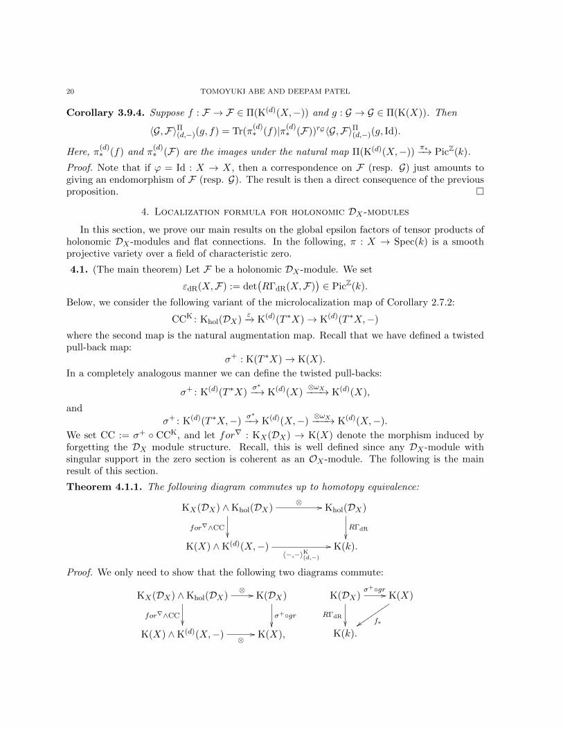
We set CC := σ+ ◦ CCK, and let for∇ : KX(DX) → K(X) denote the morphism induced byforgetting the DX module structure. Recall, this is well defined since any DX -module withsingular support in the zero section is coherent as an OX -module. The following is the mainresult of this section.
Theorem 4.1.1. The following diagram commutes up to homotopy equivalence:
KX(DX) ∧Khol(DX)⊗ //
for∇∧CC��
Khol(DX)
RΓdR
��K(X) ∧K(d)(X,−)
〈−,−〉K(d,−)
// K(k).
Proof. We only need to show that the following two diagrams commute:
KX(DX) ∧Khol(DX)⊗ //
for∇∧CC��
K(DX)
σ+◦gr��
K(X) ∧K(d)(X,−) ⊗// K(X),
K(DX)σ+◦gr //
RΓdR
��
K(X)
f∗zzuuuuuuuuu
K(k).
ON A LOCALIZATION FORMULA OF EPSILON FACTORS VIA MICROLOCAL GEOMETRY 21
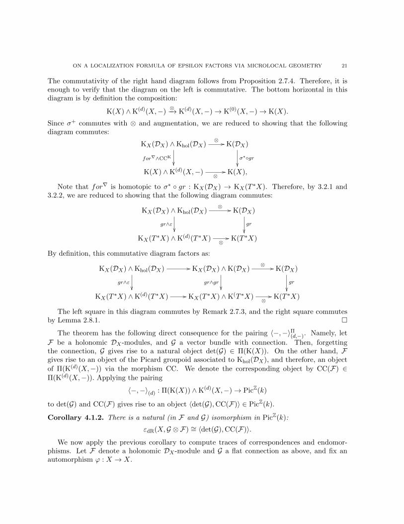
The commutativity of the right hand diagram follows from Proposition 2.7.4. Therefore, it isenough to verify that the diagram on the left is commutative. The bottom horizontal in thisdiagram is by definition the composition:
K(X) ∧K(d)(X,−)⊗−→ K(d)(X,−)→ K(0)(X,−)→ K(X).
Since σ+ commutes with ⊗ and augmentation, we are reduced to showing that the followingdiagram commutes:
KX(DX) ∧Khol(DX)⊗ //
for∇∧CCK
��
K(DX)
σ∗◦gr��
K(X) ∧K(d)(X,−) ⊗// K(X),
Note that for∇ is homotopic to σ∗ ◦ gr : KX(DX) → KX(T ∗X). Therefore, by 3.2.1 and3.2.2, we are reduced to showing that the following diagram commutes:
KX(DX) ∧Khol(DX)⊗ //
gr∧ε��
K(DX)
gr
��KX(T ∗X) ∧K(d)(T ∗X) ⊗
// K(T ∗X)
By definition, this commutative diagram factors as:
KX(DX) ∧Khol(DX) //
gr∧ε��
KX(DX) ∧K(DX)⊗ //
gr∧gr��
K(DX)
gr
��KX(T ∗X) ∧K(d)(T ∗X) // KX(T ∗X) ∧K(T ∗X) ⊗
// K(T ∗X)
The left square in this diagram commutes by Remark 2.7.3, and the right square commutesby Lemma 2.8.1. �
The theorem has the following direct consequence for the pairing 〈−,−〉Π(d,−). Namely, let
F be a holonomic DX -modules, and G a vector bundle with connection. Then, forgettingthe connection, G gives rise to a natural object det(G) ∈ Π(K(X)). On the other hand, Fgives rise to an object of the Picard groupoid associated to Khol(DX), and therefore, an object
of Π(K(d)(X,−)) via the morphism CC. We denote the corresponding object by CC(F) ∈Π(K(d)(X,−)). Applying the pairing
〈−,−〉(d) : Π(K(X)) ∧K(d)(X,−)→ PicZ(k)
to det(G) and CC(F) gives rise to an object 〈det(G),CC(F)〉 ∈ PicZ(k).
Corollary 4.1.2. There is a natural (in F and G) isomorphism in PicZ(k):
εdR(X,G ⊗ F) ∼= 〈det(G),CC(F)〉.
We now apply the previous corollary to compute traces of correspondences and endomor-phisms. Let F denote a holonomic DX -module and G a flat connection as above, and fix anautomorphism ϕ : X → X.
22 TOMOYUKI ABE AND DEEPAM PATEL
Definition 4.1.3. A correspondence ΦF on F is an isomorphism ΦF : F → ϕ∗F of DX -modules. Since ϕ is assumed to be an automorphism, this is equivalent to giving an isomorphismΨF : ϕ∗F → F .
We fix correspondences ΦF and ΨG on F and G. Note that if ϕ = id is the identity, thena correspondence is simply an automorphism. Moreover, just as in 3.9, one has an inducedcorrespondence
ΦF ⊗ΨG : F ⊗ G → ϕ∗(F ⊗ G).
It follows that one has an induced quasi-isomorphism:
RΓ(ΦF ⊗ΨG) : RΓdR(X,F ⊗ G)→ RΓdR(X,F ⊗ G).
We let εdR(X,F⊗G; ΦF⊗ΨG) := Tr(ΦF⊗ΨG : det(RΓdR(X,F⊗G)) ∈ k×. If ϕ is the identity, wehave simply automorphisms f : F → F and g : G → G (as DX -modules). In this case we denotethe corresponding epsilon factor by εdR(X,F⊗G; f⊗g) := Tr(f⊗g : det(RΓdR(X,F⊗G)) ∈ k×.In the following, we fix a lift SS(F) ∈ Z0(X) of [CC(F)] ∈ CH0(X). Moreover, we fix an object
(as in 3.9), also denote by SS(F), of Π(K(d)(X)) whose image in Π(K(d)(X,−)) is isomorphic toCC(F) and finally G0 as in 3.9.3 (corresponding to det(G) ∈ Π(K(X))). By Proposition 3.9.3,this data allows us to define 〈G0,SS(F)〉(ΨG)Π
(d,−) ∈ k×.
Theorem 4.1.4. With notation as above:
(i) One has
εdR(X,F ⊗ G; ΦF ⊗ΨG) = εdR(X,F ; ΦF )rG × 〈G0, SS(F)〉(ΨG)Π(d,−)
(ii) In the setting of endomorphisms (i.e. ϕ = id), we have
εdR(X,F ⊗ G; f ⊗ g) = εdR(X,F ; f)rG × 〈det(G), SS(F)〉(g)
Proof. The first equality follows directly from the theorem and Proposition 3.9.3. For the secondstatement, we note that in the setting of endomorphisms one has by Proposition 3.9.4:
εdR(X,F ⊗ G; f ⊗ g) = εdR(X,F ; f)rG × 〈det(G),SS(F)〉Π(d,−)(g, Id)
On the other hand, the latter is
〈det(G),SS(F)〉Π(d,−)(g, Id) = 〈det(G), SS(F)〉Π(d)(g, Id) = 〈det(G),SS(F)〉(g)
by Corollary 3.5.1. �
Remark 4.1.5. We note that CC(F) ∈ CHd(X) is precisely the pull back of the characteristiccycle of F under the zero section σ∗ : CHd(T ∗X)→ CHd(X).
4.2. (A formula for the local pairing) Let G ∈ ΠK(X), and ΨG : ϕ∗G → G be a correspondencein ΠK(X). As before, we shall let G0 denote the associated rank 0 object and ΨG0 the inducedcorrespondence. Recall, the choice of such G0 is unique up to isomorphism. Assume given acycle z ∈ CHd(X) such that z = ϕ∗(z). We take an object OZ ∈ ΠK(d)(X,−) which corresponds
to z via the isomorphism π0K(d)(X,−) ∼= CH0(X), and take a correspondence P : OZ → ϕ∗OZas well. Since z = ϕ∗(z), such a correspondence must exist (though it may not be unique).
In this setting, we have seen that in the proof of Proposition 3.9.3 that
〈G0,OZ〉Π(d,−) (ΨG0 , P ) ∈ k×
ON A LOCALIZATION FORMULA OF EPSILON FACTORS VIA MICROLOCAL GEOMETRY 23
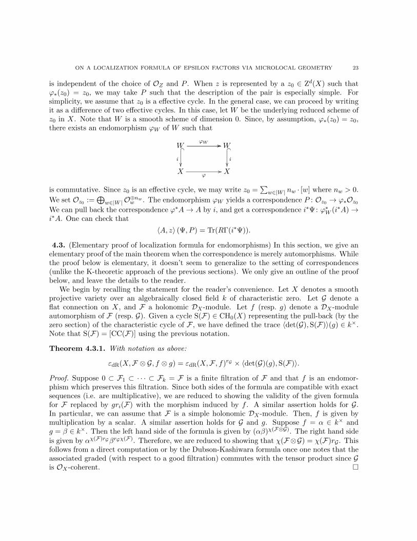
is independent of the choice of OZ and P . When z is represented by a z0 ∈ Zd(X) such thatϕ∗(z0) = z0, we may take P such that the description of the pair is especially simple. Forsimplicity, we assume that z0 is a effective cycle. In the general case, we can proceed by writingit as a difference of two effective cycles. In this case, let W be the underlying reduced scheme ofz0 in X. Note that W is a smooth scheme of dimension 0. Since, by assumption, ϕ∗(z0) = z0,there exists an endomorphism ϕW of W such that
W //� _
i��
ϕW // W� _
i��
X ϕ// X
is commutative. Since z0 is an effective cycle, we may write z0 =∑
w∈|W | nw · [w] where nw > 0.
We set Oz0 :=⊕
w∈|W |O⊕nww . The endomorphism ϕW yields a correspondence P : Oz0 → ϕ∗Oz0
We can pull back the correspondence ϕ∗A→ A by i, and get a correspondence i∗Ψ: ϕ∗W (i∗A)→i∗A. One can check that
〈A, z〉 (Ψ, P ) = Tr(RΓ(i∗Ψ)).
4.3. (Elementary proof of localization formula for endomorphisms) In this section, we give anelementary proof of the main theorem when the correspondence is merely automorphisms. Whilethe proof below is elementary, it doesn’t seem to generalize to the setting of correspondences(unlike the K-theoretic approach of the previous sections). We only give an outline of the proofbelow, and leave the details to the reader.
We begin by recalling the statement for the reader’s convenience. Let X denotes a smoothprojective variety over an algebraically closed field k of characteristic zero. Let G denote aflat connection on X, and F a holonomic DX -module. Let f (resp. g) denote a DX -moduleautomorphism of F (resp. G). Given a cycle S(F) ∈ CH0(X) representing the pull-back (by thezero section) of the characteristic cycle of F , we have defined the trace 〈det(G), S(F)〉(g) ∈ k×.Note that S(F) = [CC(F)] using the previous notation.
Theorem 4.3.1. With notation as above:
εdR(X,F ⊗ G, f ⊗ g) = εdR(X,F , f)rG × 〈det(G)(g),S(F)〉.
Proof. Suppose 0 ⊂ F1 ⊂ · · · ⊂ Fk = F is a finite filtration of F and that f is an endomor-phism which preserves this filtration. Since both sides of the formula are compatible with exactsequences (i.e. are multiplicative), we are reduced to showing the validity of the given formulafor F replaced by gri(F) with the morphism induced by f . A similar assertion holds for G.In particular, we can assume that F is a simple holonomic DX -module. Then, f is given bymultiplication by a scalar. A similar assertion holds for G and g. Suppose f = α ∈ k× andg = β ∈ k×. Then the left hand side of the formula is given by (αβ)χ(F⊗G). The right hand side
is given by αχ(F)rGβrGχ(F). Therefore, we are reduced to showing that χ(F⊗G) = χ(F)rG . Thisfollows from a direct computation or by the Dubson-Kashiwara formula once one notes that theassociated graded (with respect to a good filtration) commutes with the tensor product since Gis OX -coherent. �
24 TOMOYUKI ABE AND DEEPAM PATEL
References
[1] A. Beilinson. Topological e-factors. Pure Appl. Math. Q., 3(1, part 3):357–391, 2007.[2] P. Deligne. Le determinant de la cohomologie. In Current trends in arithmetical algebraic geometry (Arcata,
Calif., 1985), volume 67 of Contemp. Math., pages 93–177. Amer. Math. Soc., Providence, RI, 1987.[3] K. Kato and T. Saito. Ramification theory for varieties over a perfect field. Ann. of Math. (2), 168(1):33–96,
2008.[4] F.F. Knudsen. Determinant functors on exact categories and their extensions to categories of bounded com-
plexes. Michigan Math. J., 50(2):407–444, 2002.[5] F.F Knudsen and D. Mumford. The projectivity of the moduli space of stable curves. I. Preliminaries on
“det” and “Div”. Math. Scand., 39(1):19–55, 1976.[6] M. Levine. Chow’s moving lemma and the homotopy coniveau tower. K-Theory, 37(1-2):129–209, 2006.[7] M. Levine. The homotopy coniveau tower. J. Topol., 1(1):217–267, 2008.[8] D. Patel. de Rham D-factors. Invent. Math., 190(2):299–355, 2012.[9] S. Schwede. Symmetric spectra. preprint.
[10] R.W. Thomason and T. Trobaugh. Higher algebraic K-theory of schemes and of derived categories. In TheGrothendieck Festschrift, Vol. III, volume 88 of Progr. Math., pages 247–435. Birkhauser Boston, Boston,MA, 1990.
[11] N. Umezaki, E. Yang, and Y. Zhao. Characteristic class and the ε-factor of an etale sheaf. preprint.
Kavli IPMU (WPI), UTIAS, The University of Tokyo, Kashiwa, Chiba 277-8583, JapanE-mail address: [email protected]
Department of Mathematics, Purdue University, 150 N. University Street, West Lafayette, IN47907, U.S.A.
E-mail address: [email protected]