Numerical methods and arbitrary-precision computation of ...
Constructive Computation Theory
Gerard Huet
An executable computability theory course
based on λ-calculus
August 2011

Version 11-08-2011
c©G. Huet 1992–2011
Contents
1 λ-calculus: Syntax and Computation strategies 71.1 Abstract syntax . . . . . . . . . . . . . . . . . . . . . . . . . . . . . . . . . . . . . . 71.2 Concrete syntax: pure λ-expressions . . . . . . . . . . . . . . . . . . . . . . . . . . 9
1.2.1 λ-expressions . . . . . . . . . . . . . . . . . . . . . . . . . . . . . . . . . . . 91.2.2 Parsing . . . . . . . . . . . . . . . . . . . . . . . . . . . . . . . . . . . . . . 91.2.3 Unparsing . . . . . . . . . . . . . . . . . . . . . . . . . . . . . . . . . . . . . 101.2.4 Grammar . . . . . . . . . . . . . . . . . . . . . . . . . . . . . . . . . . . . . 101.2.5 Printer . . . . . . . . . . . . . . . . . . . . . . . . . . . . . . . . . . . . . . . 12
1.3 Substitution . . . . . . . . . . . . . . . . . . . . . . . . . . . . . . . . . . . . . . . . 131.4 A theory of substitution . . . . . . . . . . . . . . . . . . . . . . . . . . . . . . . . . 15
1.4.1 Contextual induction . . . . . . . . . . . . . . . . . . . . . . . . . . . . . . . 151.4.2 A more explicit formulation of subst. . . . . . . . . . . . . . . . . . . . . . . 151.4.3 Formal properties of substitution . . . . . . . . . . . . . . . . . . . . . . . . 15
1.5 Computation strategies . . . . . . . . . . . . . . . . . . . . . . . . . . . . . . . . . 161.5.1 Normal order . . . . . . . . . . . . . . . . . . . . . . . . . . . . . . . . . . . 161.5.2 Applicative order . . . . . . . . . . . . . . . . . . . . . . . . . . . . . . . . . 18
1.6 Conversion . . . . . . . . . . . . . . . . . . . . . . . . . . . . . . . . . . . . . . . . 19
2 Computability theory based on λ-calculus 212.1 Church’s encoding of arithmetic . . . . . . . . . . . . . . . . . . . . . . . . . . . . . 21
2.1.1 Booleans . . . . . . . . . . . . . . . . . . . . . . . . . . . . . . . . . . . . . 212.1.2 Naturals . . . . . . . . . . . . . . . . . . . . . . . . . . . . . . . . . . . . . . 212.1.3 Arithmetic operations . . . . . . . . . . . . . . . . . . . . . . . . . . . . . . 222.1.4 Primitive recursion . . . . . . . . . . . . . . . . . . . . . . . . . . . . . . . . 232.1.5 Functional iteration . . . . . . . . . . . . . . . . . . . . . . . . . . . . . . . 242.1.6 General recursion . . . . . . . . . . . . . . . . . . . . . . . . . . . . . . . . . 252.1.7 Turing completeness . . . . . . . . . . . . . . . . . . . . . . . . . . . . . . . 25
2.2 λ-calculus as a general programming language . . . . . . . . . . . . . . . . . . . . . 252.2.1 Lists . . . . . . . . . . . . . . . . . . . . . . . . . . . . . . . . . . . . . . . . 262.2.2 Complexity considerations . . . . . . . . . . . . . . . . . . . . . . . . . . . . 282.2.3 Recursive naturals . . . . . . . . . . . . . . . . . . . . . . . . . . . . . . . . 282.2.4 Other representations . . . . . . . . . . . . . . . . . . . . . . . . . . . . . . 30
2.3 Rudiments of recursion theory . . . . . . . . . . . . . . . . . . . . . . . . . . . . . . 312.3.1 Godel’s numberings . . . . . . . . . . . . . . . . . . . . . . . . . . . . . . . 312.3.2 The Rice-Scott theorem . . . . . . . . . . . . . . . . . . . . . . . . . . . . . 32
3 Confluence of reduction 333.1 Positions, subterms . . . . . . . . . . . . . . . . . . . . . . . . . . . . . . . . . . . . 33
3.1.1 Positions . . . . . . . . . . . . . . . . . . . . . . . . . . . . . . . . . . . . . 333.1.2 Subterms . . . . . . . . . . . . . . . . . . . . . . . . . . . . . . . . . . . . . 35
3.2 Reduction . . . . . . . . . . . . . . . . . . . . . . . . . . . . . . . . . . . . . . . . . 363.2.1 Redexes . . . . . . . . . . . . . . . . . . . . . . . . . . . . . . . . . . . . . . 36
3
4 CONTENTS
3.2.2 β-reduction and conversion . . . . . . . . . . . . . . . . . . . . . . . . . . . 363.2.3 Leftmost-outermost strategy . . . . . . . . . . . . . . . . . . . . . . . . . . 383.2.4 Residuals . . . . . . . . . . . . . . . . . . . . . . . . . . . . . . . . . . . . . 39
3.3 Sets of redexes as marked λ-terms . . . . . . . . . . . . . . . . . . . . . . . . . . . 413.3.1 Redexes as terms with extra structure . . . . . . . . . . . . . . . . . . . . . 413.3.2 The Boolean algebra of mutually compatible redexes . . . . . . . . . . . . . 443.3.3 Glueing together reduction and residuals . . . . . . . . . . . . . . . . . . . . 443.3.4 The Prism Theorem and the Cube Lemma . . . . . . . . . . . . . . . . . . 45
3.4 Parallel derivations . . . . . . . . . . . . . . . . . . . . . . . . . . . . . . . . . . . . 463.5 Residual algebra . . . . . . . . . . . . . . . . . . . . . . . . . . . . . . . . . . . . . 473.6 The derivations lattice . . . . . . . . . . . . . . . . . . . . . . . . . . . . . . . . . . 483.7 Single derivations . . . . . . . . . . . . . . . . . . . . . . . . . . . . . . . . . . . . . 50
4 Derivation induction and standardisation 514.1 Residual derivations . . . . . . . . . . . . . . . . . . . . . . . . . . . . . . . . . . . 514.2 Developments . . . . . . . . . . . . . . . . . . . . . . . . . . . . . . . . . . . . . . . 524.3 Proof of the finite development theorem . . . . . . . . . . . . . . . . . . . . . . . . 53
4.3.1 Weighted terms . . . . . . . . . . . . . . . . . . . . . . . . . . . . . . . . . . 534.3.2 Decreasing weighted terms . . . . . . . . . . . . . . . . . . . . . . . . . . . 55
4.4 Induction on derivations . . . . . . . . . . . . . . . . . . . . . . . . . . . . . . . . . 564.4.1 Redexes contributing fully to a derivation . . . . . . . . . . . . . . . . . . . 564.4.2 Derivations contraction . . . . . . . . . . . . . . . . . . . . . . . . . . . . . 57
4.5 Standardisation . . . . . . . . . . . . . . . . . . . . . . . . . . . . . . . . . . . . . . 584.5.1 Residuals of outer redexes . . . . . . . . . . . . . . . . . . . . . . . . . . . . 584.5.2 Standard derivations . . . . . . . . . . . . . . . . . . . . . . . . . . . . . . . 594.5.3 Standardisation . . . . . . . . . . . . . . . . . . . . . . . . . . . . . . . . . . 604.5.4 Correctness of the normal strategy . . . . . . . . . . . . . . . . . . . . . . . 61
5 Separability 635.1 Extensionality: η-conversion . . . . . . . . . . . . . . . . . . . . . . . . . . . . . . . 635.2 Head normal forms and solvability . . . . . . . . . . . . . . . . . . . . . . . . . . . 64
5.2.1 Head normal forms . . . . . . . . . . . . . . . . . . . . . . . . . . . . . . . . 645.2.2 Solvability . . . . . . . . . . . . . . . . . . . . . . . . . . . . . . . . . . . . . 645.2.3 A normal interpreter . . . . . . . . . . . . . . . . . . . . . . . . . . . . . . . 65
5.3 Bohm trees . . . . . . . . . . . . . . . . . . . . . . . . . . . . . . . . . . . . . . . . 655.4 Bohm’s Theorem . . . . . . . . . . . . . . . . . . . . . . . . . . . . . . . . . . . . . 67
5.4.1 Separability . . . . . . . . . . . . . . . . . . . . . . . . . . . . . . . . . . . . 675.4.2 Accessibility in Bohm trees . . . . . . . . . . . . . . . . . . . . . . . . . . . 675.4.3 A Bohm-out toolkit . . . . . . . . . . . . . . . . . . . . . . . . . . . . . . . 695.4.4 Semi-separability . . . . . . . . . . . . . . . . . . . . . . . . . . . . . . . . . 715.4.5 Separating non-similar approximations . . . . . . . . . . . . . . . . . . . . . 715.4.6 The Bohm-out algorithm . . . . . . . . . . . . . . . . . . . . . . . . . . . . 725.4.7 The separability theorem . . . . . . . . . . . . . . . . . . . . . . . . . . . . 745.4.8 Searching for a separating path . . . . . . . . . . . . . . . . . . . . . . . . . 755.4.9 Left Bohm separator . . . . . . . . . . . . . . . . . . . . . . . . . . . . . . . 76
5.5 To know more . . . . . . . . . . . . . . . . . . . . . . . . . . . . . . . . . . . . . . . 77
Introduction
We give in these notes an overview of computation theory, presented in the paradigm of λ-calculus. The descriptive formalism used is not the usual meta-language of Mathematics, butan actual programming language, Pidgin ML, a variant of Objective Caml, developed at theParis-Rocquencourt INRIA center. This has the double advantage of being more rigorous, moreconstructive, and of allowing better understanding by the reader who may interactively executeall definitions and examples of the course. The corresponding programs may be downloaded fromthe site http://yquem.inria.fr/~huet/CCT/. The programs may be executed with ObjectiveCaml, version 3.12 (See http://caml.inria.fr/ocaml/index.html).
A previous version of these notes in French was circulated between 1988 and 1991 underthe name: “Initiation au λ-calcul.” It formed the notes of a graduate course for the “DEAd’Informatique Fondamentale” at Universite Paris VII. The next version formed the λ-calculusportion of a course on Functional Programming given by the author at the Computer ScienceDivision of AIT, Bangkok (Thailand), from January to March 1992. The support of AIT isgratefully acknowledged. An update was prepared for the “Ecole Jeunes Chercheurs du Greco deProgrammation”, Bordeaux, April 1992, and revised as notes for a course on λ-calculus for theDEA Informatique, Mathematiques et Applications, taught at ENS in Paris during Fall 1992 and1993, for the DEA Fonctionnalite et Theorie des Types, Universite Paris 7 in 1994. This coursewas taught again in the DEA d’Informatique de l’Universite Bordeaux I in 2002. This course waslast taught at the MPRI (Master Parisien de Recherche en Informatique) in Paris in 2004. TheML code was revised in 2011 in order to adapt to Ocaml 3.12.
The author is grateful for any comment/criticism of this work, which may be communicatedby electronic mail at [email protected].
5

6 CONTENTS
Chapter 1
λ-calculus: Syntax andComputation strategies
We consider in this chapter pure λ-calculus. It is the basic formalism to describe functions, ormore precisely algorithms, and to discuss their computations.
First we consider λ-expressions. There are three constructors of such functional expressions:variables such as x, applications of an expression e1 to an expression e2, written (e1 e2), andfinally functional abstraction of an expression ex over a variable x considered as its formal param-eter, traditionally written λx · ex, but for which we shall use the notation [x]ex. This notationstands for the algorithm which computes the value of expression ex, given an input argument x.
Abstraction is a binding operation: its formal parameter x is bound in [x]ex. Such boundvariables are dummies, in that their name does not matter, and thus [x]ex is the same as say[y]ey, where ey is ex, in which every free occurrence of x is replaced by y. Here we have twodifficulties in explaining this renaming operation as an expression morphism. First, there is the“free” restriction above, due to the fact that we may rebind the same x in its own scope. Secondly,the choice of y is constrained by possible bindings in an outer scope. Thus, [y][x](x y) isdefinitely not the same as [y][y](y y): in the latter, the free occurrence of y has been “captured”by the inner abstraction, an undesirable effect. The traditional presentation spends a considerableeffort in explaining the legal conditions under which renaming is permitted (the so-called α-conversion rule), and this explanation is left at the level of the meta-language, which prevents atthe outset formal proof methods such as structural induction.
It may be useful to remark here that it is definitely not enough to assume that the initialterm of some computation has distinct names for all its bound variables, since this property isnot preserved by reduction, as the reader may easily convince himself by contemplating the term([z](z z) [y][x](y x)).
We shall deal immediately with this difficulty, by defining a proper abstract syntax wherevariables are not represented as actual identifier strings, but rather as reference indexes identifyingcanonically their binding abstractor. We shall use consistently the name term for an abstractsyntax construction, and expression for a concrete syntax construction.
1.1 Abstract syntax
The abstract syntax of λ-terms is defined as an ML inductive type term as follows:
# type term =
[ Ref of int (* variables as reference depth *)
| Abs of term (* abstraction [x]t *)
| App of term and term (* application (t u) *)
];
7
8 CHAPTER 1. λ-CALCULUS: SYNTAX AND COMPUTATION STRATEGIES
type term = [ Ref of int | Abs of term | App of term and term ]
Such definitions have two parts. The first part, starting with the sharp symbol # (the MLprompt symbol), and ending with a semicolon, is the definition proper. Such definitions areanalysed by the ML compiler, typed-checked, and the result of this analysis is given in the secondpart. In the case of the declaration of a value, computation takes place, and the value producedis printed by ML with its type. When the value is too big, we write ... to abbreviate it. Thesymbol <fun> is ML’s own way to abbreviate a closure (functional value), which has no concreterepresentation.
Let us comment on the three constructors of type term. (App f x) represents the application offunction f to argument x. If f is an expression containing a free variable u, then the function whichassociates f to its formal argument x, noted [u]f in concrete syntax, is represented abstractly as(Abs f). Finally, a (Ref n) node designates the variable declared in the nth Abs binder aboveit, in the de Bruijn index tradition [3]. This corresponds to variables designating indexes in thestatic environment.
A λ-term is valid in any context deep enough to represent its free variables. More precisely,a term t is valid in a context of n free variables iff (valid_at_depth n t) as defined below.
Note. What we exactly mean by this statement is the following. The ML sentence below definesan algorithm valid_at_depth of type int -> term -> bool. For every integer value n, andevery well-formed term t, the computation of (valid_at_depth n t) terminates with a booleanvalue b, since the recursive definition is well-founded (it uses structural induction on t). Thus weexplain that t is valid in a context of n free variables iff (valid_at_depth n t) evaluates to theML boolean value True. Actually in all that follows we shall use non-negative integers for referenceindexes, and thus (Ref n) will be well-formed only when n ≥ 0. Similarly, the first argument offunction valid_at_depth should be non-negative. This is typical of the approach taken here: thetype discipline of ML insures that the functions defined as ML algorithms compute functions ofthe appropriate type, but the totality of such functions on a domain which may be a subset ofthe values of the corresponding type, as well as other correctness assertions, must be argued ininformal mathematics. We thus consider that these notes represent a pre-formal development ofthe subject matter. We leave it as a promising challenge for formalists to extract these algorithmsfrom mechanically verified formal proofs of consistency of their specifications. Actually, some partsof the current notes have already been formalised in the Coq proof assistant [6].
# value rec valid_at_depth n = fun
[ Ref m -> m < n
| Abs t -> valid_at_depth (n+1) t
| App t u -> valid_at_depth n t && valid_at_depth n u
];
value valid_at_depth : int -> term -> bool = <fun>
A closed λ-term is valid in an empty context, i.e. it does not contain free variables. We shall alsocall combinator a closed term.
# value closed_term = valid_at_depth 0;
value closed_term : term -> bool = <fun>
Note that (valid_at_depth n t) implies (closed_term (abstract n t)), where abstract
iterates the wrapping of its argument with the Abs constructor (an easy programming exercise leftto the reader). Every term has a minimum context depth:
# value min_context_depth = min_rec 0
where rec min_rec n = fun
[ Ref m -> m-n+1
| Abs t -> min_rec (n+1) t
1.2. CONCRETE SYNTAX: PURE λ-EXPRESSIONS 9
| App t u -> max (min_rec n t) (min_rec n u)
];
value min_context_depth : Term.term -> int = <fun>
# value abs t = Abs t
and app f x = App f x;
value abs : Term.term -> Term.term = <fun>
value app : Term.term -> Term.term -> Term.term = <fun>
# value rec iter f n x = if n=0 then x else iter f (n-1) (f x);
value iter : (’a -> ’a) -> int -> ’a -> ’a = <fun>
# value abstract n = iter abs n;
value abstract : int -> Term.term -> Term.term = <fun>
# value closure t = abstract (min_context_depth t) t;
value closure : Term.term -> Term.term = <fun>
Fact. The closure of a λ-term is a closed_term.
1.2 Concrete syntax: pure λ-expressions
We shall now define a concrete syntax for λ-expressions, in order to read and write λ-terms usingvariable names as usual.
1.2.1 λ-expressions
We shall now define concrete λ-expressions, where variables are named by identifier strings. Suchexpressions with free variables are given abstract meaning with the help of an environment:
# type environment = list string;
We assume an error routine which raises a qualified exception.
# value error message = raise (Failure message)
and fail () = raise (Failure "");
value error : string -> ’a = <fun>
value fail : unit -> ’a = <fun>
Here is now the type of concrete λ-expressions.
# type expression =
[ Var of string
| Lambda of string and expression
| Apply of expression and expression
];
1.2.2 Parsing
The next function computes a reference index in an environment.
value index_of (id:string) = search 0
where rec search n = fun
[ [ name :: names ] -> if name=id then n
else search (n+1) names
| [] -> error "Unbound identifier"
];
value index_of : string -> list string -> int = <fun>
10 CHAPTER 1. λ-CALCULUS: SYNTAX AND COMPUTATION STRATEGIES
We parse λ-terms in an environment lvars with function parse_env:
# value rec parse_env env = abstract
where rec abstract = fun
[ Var name -> try Ref (index_of name env)
with [ (Failure _) -> error "Expression not closed" ]
| Lambda id conc -> Abs (parse_env [ id :: env ] conc)
| Apply conc1 conc2 -> App (abstract conc1) (abstract conc2)
];
value parse_env : list string -> expression -> Term.term = <fun>
The parser parses closed λ-expressions.
# value parse = parse_env [];
value parse : expression -> Term.term = <fun>
1.2.3 Unparsing
As unparsing convention, we print bound variables as x0, x1, etc., and free variables as u0, u1,etc.
# value bound_var n = "x" ^ string_of_int n
and free_var n = "u" ^ string_of_int n;
value bound_var : int -> string = <fun>
value free_var : int -> string = <fun>
We now obtain a term from an expression in an environment:
# value expression free_vars = expr free_vars (List.length free_vars)
where rec expr env depth = fun
[ Ref n -> Var (if n>=depth then free_var(n-depth)
else List.nth env n)
| App u v -> Apply (expr env depth u) (expr env depth v)
| Abs t -> let x = bound_var depth
in Lambda x (expr [x::env] (depth+1) t)
];
value expression : list string -> Term.term -> expression = <fun>
We get an unparser from closed λ-terms to concrete λ-expressions as:
# value unparse = expression [];
value unparse : Term.term -> expression = <fun>
1.2.4 Grammar
We now give the grammar for concrete λ-expressions. For readers not familiar with the Ocam-l/Camlp4 convention for describing grammars, just read the rules names as non-terminals, theirleft-hand side as BNF rules, and their right-hand sides as semantic actions computing synthesisedattributes.
module Gram = MakeGram Lexer;
value term_exp_eoi = Gram.Entry.mk "term"
and expr_exp_eoi = Gram.Entry.mk "lambda";
EXTEND Gram
GLOBAL: term_exp_eoi expr_exp_eoi;
1.2. CONCRETE SYNTAX: PURE λ-EXPRESSIONS 11
term_exp_eoi:
[ [ e = expr_exp_eoi -> <:expr< Expression.parse $e$ >> ] ];
expr_exp_eoi:
[ [ e = expr_exp; ‘EOI -> e ] ];
expr_exp:
[ [ "["; b = binder; "]"; e = expr_exp
-> let func v e = <:expr< Lambda $str:v$ $e$ >> in
List.fold_right func b <:expr<$e$>>
| "("; appl = lexpr_exp; ")" -> appl
| x = LIDENT -> <:expr< Var $str:x$ >>
| "let"; x = LIDENT; "="; e1 = expr_exp; "in"; e2 = expr_exp
-> <:expr< Apply (Lambda $str:x$ $e2$) $e1$ >>
| "!"; x = exp_antiquot -> <:expr< Expression.unparse $x$ >>
] ];
lexpr_exp:
[ [ e = expr_exp -> e
| l = lexpr_exp; e = expr_exp -> <:expr< Apply $l$ $e$ >>
] ];
binder:
[ [ x = LIDENT -> [ x ]
| x = LIDENT; ","; b = binder -> [ x :: b ]
] ];
exp_antiquot:
[ [ x = UIDENT ->
<:expr< $lid: "_" ^ x $ >>
] ];
END;
value expr_exp = Gram.parse_string expr_exp_eoi
and term_exp = Gram.parse_string term_exp_eoi;
value expand_expr loc _ s = expr_exp loc s
and expand_term loc _ s = term_exp loc s
and expand_str_item_expr loc _ s = <:str_item@loc< $exp:expr_exp loc s$ >>
and expand_str_item_term loc _ s = <:str_item@loc< $exp:term_exp loc s$ >>
;
Quotation.add "expr" Quotation.DynAst.expr_tag expand_expr;
Quotation.add "term" Quotation.DynAst.expr_tag expand_term;
Quotation.add "expr" Quotation.DynAst.str_item_tag expand_str_item_expr;
Quotation.add "term" Quotation.DynAst.str_item_tag expand_str_item_term;
Quotation.default.val := "term";
For instance :
#<:expr<[x](x [y](x y))>>;
- : Expression.expression =
Lambda "x" (Apply (Var "x") (Lambda "y" (Apply (Var "x") (Var "y"))))
#<:term<[x](x [y](x y))>>;
- : Term.term =
Abs (App (Ref 0) (Abs (App (Ref 1) (Ref 0))))
We invite the reader to examine carefully the value returned by this expression in order tounderstand de Bruijn’s notation. (Ref 1) refers to the variable which is bound in the 2nd Abs
node above it in the λ-term. Thus the two occurrences of variable x get assigned different indexes,since the second one has to cross y’s binder in order to point to its own. Conversely, the two sub-
12 CHAPTER 1. λ-CALCULUS: SYNTAX AND COMPUTATION STRATEGIES
terms (Ref 0) refer to distinct variables. Abstract syntax is the adequate structure for reasoningstructurally about λ-terms, but it is not convenient as notation for humans.
This grammar allows only the parsing of closed terms. In order to parse a concrete expressionexpr containing free variables x and y, encapsulate it with an appropriate context, like in:
# match <<[x,y](x y)>> with [ Abs(Abs(t)) -> t | _ -> fail() ];
- : Term.term = App (Ref 1) (Ref 0)
Remark that applications associate to the left, whereas abstractions associate to the right.Thus [x,y,z](x y z) abbreviates [x][y][z]((x y) z). Note that the ML “let” notation isintroduced as a macro generator for terms of the form App (Abs t s). Such terms, called redexes,(redex being an abbreviation for reducible expression), are subterms where some computation maytake place, as we shall see later.
The grammar rules above allow anti-quotations with the exclamation mark as follows. If _Xis an ML variable bound to a term value, the concrete expression << ... !X ... >> will insertthis value as the corresponding subterm in the parse of the expression. This facility will be usedextensively in the examples below in order to name usual combinators (closed λ-terms).
Let us now give as examples the standard combinators:
# value _I = <<[x]x>> (* Identity *)
and _K = <<[x,y]x>> (* Constant generator (Kestrel) *)
and _S = <<[x,y,z](x z (y z))>> (* Shonfinkel’s composition (Stirling) *)
and _A = <<[f,x](f x)>> (* Application *)
and _B = <<[f,g,x](f (g x))>> (* Composition *)
and _C = <<[f,x,y](f y x)>>; (* Transposition *)
value _I : Term.term = Abs (Ref 0)
value _K : Term.term = Abs (Abs (Ref 1))
...
Exercice. Other conventions for naming variables unambiguously may be devised. For instance,a variable occurrence may be represented by the position of its binder indexed from the top ofthe term, rather than relatively to the occurrence. This “dual de Bruijn’s scheme” is closer to theconcrete notation, but presents other difficulties. Compare the two schemes from the algorithmicpoint of view, in particular for the substitution operation defined in the next section.
1.2.5 Printer
We now give a simple pretty-printer of λ-terms:
value rec print_term t = print_rec [] 0 t
where rec print_rec env depth = printer True
where rec printer flag = fun
[ Ref n -> printf "%s" (if n>=depth then free_var (n-depth)
else List.nth env n)
| App u v ->
let pr_app u v = do { printer False u; printf " "; printer True v } in
if flag then do { printf "@[<1>("; pr_app u v; printf ")@]" }
else pr_app u v
| abs -> let (names,body) = peel depth [] abs in
do { print_binder (List.rev names)
; print_rec (names @ env) (depth+List.length names) body
}
]
and peel depth names = fun
[ Abs t -> let name = bound_var depth
1.3. SUBSTITUTION 13
in peel (depth+1) [ name :: names ] t
| other -> (names,other)
]
and print_binder = fun
[ [] -> ()
| [x::rest] -> do
{ printf "@[<1>[%s" x
; List.iter (fun x -> printf ",%s" x) rest
; printf "]@]"
}
];
Now ML knows how to print terms consistently with the input grammar. Thus:
#print_term <<([x,y](x (y [x]x)) [u](u u) [v,w]v)>>;
([x0,x1](x0 (x1 [x2]x2)) [x0](x0 x0) [x0,x1]x0)- : unit = ()
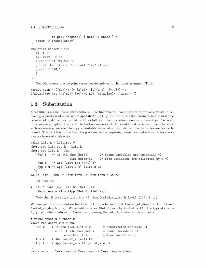
1.3 Substitution
λ-calculus is a calculus of substitutions. The fundamental computation primitive consists in re-placing a position of some redex App(Abs(t),s) by the result of substituting s to the first freevariable of t, defined as (subst s t) as follows. This operation consists in two steps. We needto recursively explore t in order to find occurrences of the substituted variable. Then, for eachsuch occurrence, we need to copy s, suitably adjusted so that its own free variables are correctlybound. The next function solves this problem, by recomputing references of global variables acrossn extra levels of abstraction.
value lift n = lift_rec 0
where rec lift_rec k = lift_k
where rec lift_k = fun
[ Ref i -> if i<k then Ref(i) (* bound variables are invariant *)
else Ref(n+i) (* free variables are relocated by n *)
| Abs t -> Abs (lift_rec (k+1) t)
| App t u -> App (lift_k t) (lift_k u)
];
value lift : int -> Term.term -> Term.term = <fun>
For instance:
# lift 1 (Abs (App (Ref 0) (Ref 1)));
- : Term.term = (Abs (App (Ref 0) (Ref 2)))
Note that if (valid_at_depth n t), then (valid_at_depth (n+k) (lift k t)).
We now give the substitution function. Let n,t, s be such that (valid_at_depth (n+1) t) and(valid_at_depth n s). We substitute s for (Ref 0) in t by (subst s t). The typical case is([x]t u), which reduces to (subst s t), using the rule of β-reduction given below.
# value subst w = subst_w 0
where rec subst_w n = fun
[ Ref k -> if k=n then lift n w (* substituted variable *)
else if k<n then Ref k (* bound variables *)
else Ref (k-1) (* free variables *)
| Abs t -> Abs (subst_w (n+1) t)
| App t u -> App (subst_w n t) (subst_w n u)
];
value subst : Term.term -> Term.term -> Term.term = <fun>
14 CHAPTER 1. λ-CALCULUS: SYNTAX AND COMPUTATION STRATEGIES
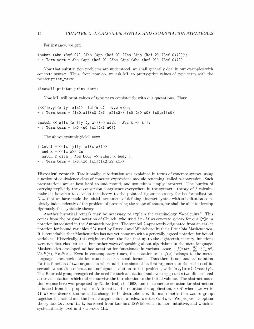
For instance, we get:
#subst (Abs (Ref 0)) (Abs (App (Ref 0) (Abs (App (Ref 2) (Ref 0)))));
- : Term.term = Abs (App (Ref 0) (Abs (App (Abs (Ref 0)) (Ref 0))))
Now that substitution problems are understood, we shall generally deal in our examples withconcrete syntax. Thus, from now on, we ask ML to pretty-print values of type term with theprinter print_term:
#install_printer print_term;
Now ML will print values of type term consistently with our quotations. Thus:
#<<([x,y](x (y [x]x)) [u](u u) [v,w]v)>>;
- : Term.term = ([x0,x1](x0 (x1 [x2]x2)) [x0](x0 x0) [x0,x1]x0)
#match <<[z][x](z ([y](y z)))>> with [ Abs t -> t ];
- : Term.term = [x0](u0 [x1](x1 u0))
The above example yields now:
# let f = <<[x][y](y [z](x z))>>
and x = <<[z]z>> in
match f with [ Abs body -> subst x body ];
- : Term.term = [x0](x0 [x1]([x2]x2 x1))
Historical remark. Traditionally, substitution was explained in terms of concrete syntax, usinga notion of equivalence class of concrete expressions modulo renaming, called α-conversion. Suchpresentations are at best hard to understand, and sometimes simply incorrect. The burden ofcarrying explicitly the α-conversion congruence everywhere in the syntactic theory of λ-calculusmakes it hopeless to develop the theory to the point of rigour necessary for its formalisation.Now that we have made the initial investment of defining abstract syntax with substitution com-pletely independently of the problem of preserving the scope of names, we shall be able to developrigorously this syntactic theory.
Another historical remark may be necessary to explain the terminology “λ-calculus.” Thiscomes from the original notation of Church, who used λx ·M as concrete syntax for our [x]M, anotation introduced in the Automath project. The symbol λ apparently originated from an earliernotation for bound variables xM used by Russell and Whitehead in their Principia Mathematica.It is remarkable that Mathematics has not yet come up with a generally agreed notation for boundvariables. Historically, this originates from the fact that up to the eighteenth century, functionswere not first-class citizens, but rather ways of speaking about algorithms in the meta-language.Mathematics developed ad-hoc notation for functionals in various areas:
∫f(x)dx, ∂f
∂x ,∑
n n2,
∀x.P (x), ∃x.P (x). Even in contemporary times, the notation x 7→ f(x) belongs to the meta-language, since such notation cannot occur as a sub-formula. Thus there is no standard notationfor the function of two arguments which adds the sinus of its first argument to the cosinus of itssecond. λ-notation offers a non-ambiguous solution to this problem, with [x,y]sin(x)+cos(y).The Bourbaki group recognised the need for such a notation, and even suggested a two-dimensionalabstract notation, which did not survive the introduction to the initial volume. The abstract nota-tion we use here was proposed by N. de Bruijn in 1968, and the concrete notation for abstractionis issued from his proposal for Automath. His notation for application, <x>f where we write(f x) was deemed too radical a change to be desirable here. Its main motivation was to grouptogether the actual and the formal arguments in a redex, written <s>[x]t. We propose as optionthe syntax let x=s in t, borrowed from Landin’s ISWIM which is more intuitive, and which issystematically used in it successor ML.
1.4. A THEORY OF SUBSTITUTION 15
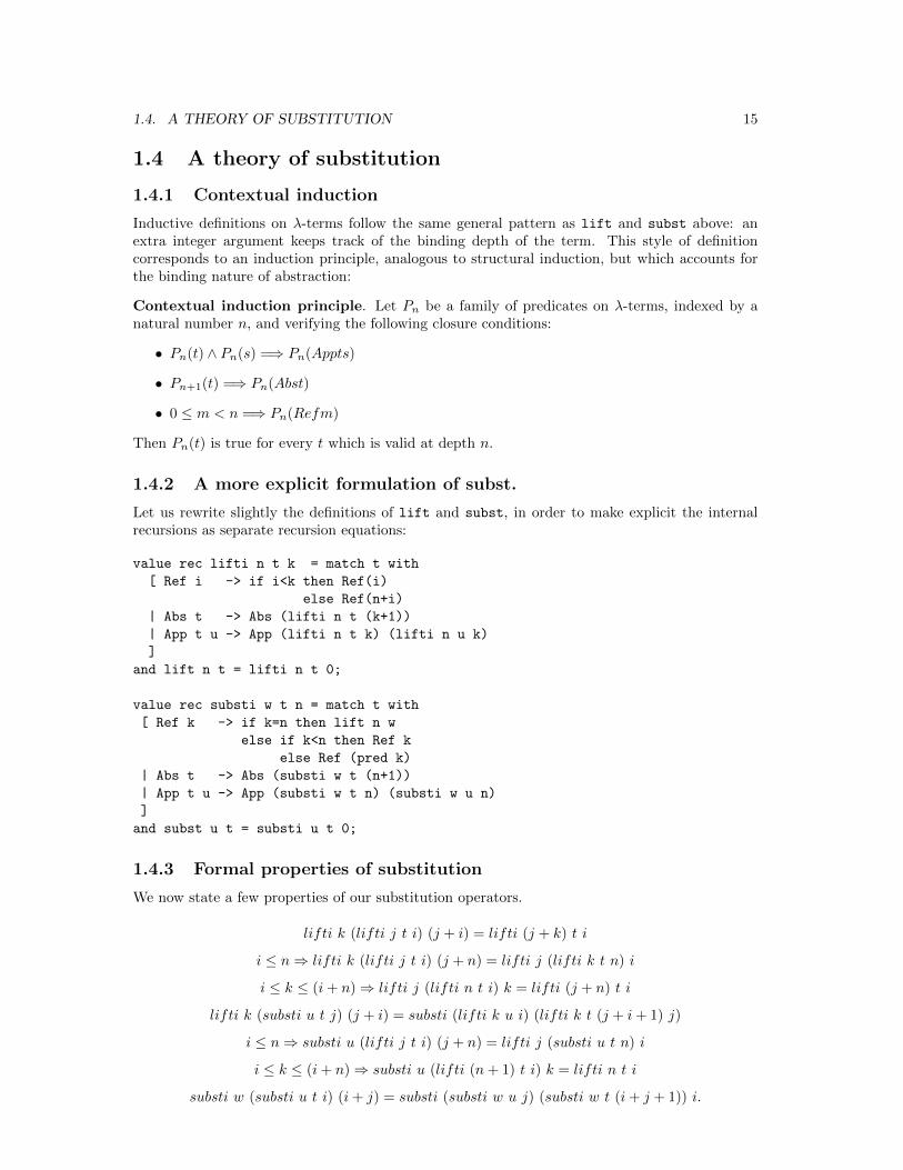
1.4 A theory of substitution
1.4.1 Contextual induction
Inductive definitions on λ-terms follow the same general pattern as lift and subst above: anextra integer argument keeps track of the binding depth of the term. This style of definitioncorresponds to an induction principle, analogous to structural induction, but which accounts forthe binding nature of abstraction:
Contextual induction principle. Let Pn be a family of predicates on λ-terms, indexed by anatural number n, and verifying the following closure conditions:
• Pn(t) ∧ Pn(s) =⇒ Pn(Appts)
• Pn+1(t) =⇒ Pn(Abst)
• 0 ≤ m < n =⇒ Pn(Refm)
Then Pn(t) is true for every t which is valid at depth n.
1.4.2 A more explicit formulation of subst.
Let us rewrite slightly the definitions of lift and subst, in order to make explicit the internalrecursions as separate recursion equations:
value rec lifti n t k = match t with
[ Ref i -> if i<k then Ref(i)
else Ref(n+i)
| Abs t -> Abs (lifti n t (k+1))
| App t u -> App (lifti n t k) (lifti n u k)
]
and lift n t = lifti n t 0;
value rec substi w t n = match t with
[ Ref k -> if k=n then lift n w
else if k<n then Ref k
else Ref (pred k)
| Abs t -> Abs (substi w t (n+1))
| App t u -> App (substi w t n) (substi w u n)
]
and subst u t = substi u t 0;
1.4.3 Formal properties of substitution
We now state a few properties of our substitution operators.
lifti k (lifti j t i) (j + i) = lifti (j + k) t i
i ≤ n⇒ lifti k (lifti j t i) (j + n) = lifti j (lifti k t n) i
i ≤ k ≤ (i+ n)⇒ lifti j (lifti n t i) k = lifti (j + n) t i
lifti k (substi u t j) (j + i) = substi (lifti k u i) (lifti k t (j + i+ 1) j)
i ≤ n⇒ substi u (lifti j t i) (j + n) = lifti j (substi u t n) i
i ≤ k ≤ (i+ n)⇒ substi u (lifti (n+ 1) t i) k = lifti n t i
substi w (substi u t i) (i+ j) = substi (substi w u j) (substi w t (i+ j + 1)) i.
16 CHAPTER 1. λ-CALCULUS: SYNTAX AND COMPUTATION STRATEGIES
These technical lemmas are intermediary steps in the proof of the substitution theorem, whichexpresses that substitution distributes:
Substitution Theorem. For every terms M,N,P , for every index n ≥ 0:
substi P (subst N M) n = subst (substi P N n) (substi P M (n+ 1)).
This theorem is formally proved in [6], using the Calculus of Inductive Constructions. Thisproof has been mechanically verified by the Coq proof assistant (http://coq.inria.fr).
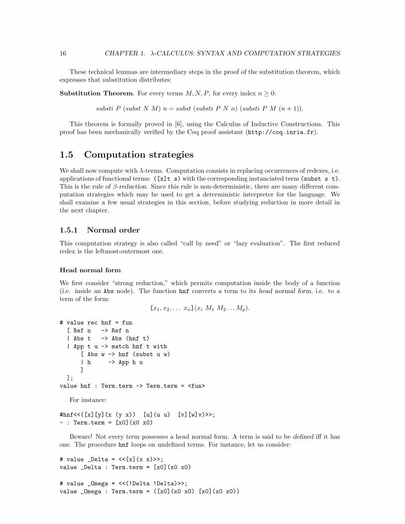
1.5 Computation strategies
We shall now compute with λ-terms. Computation consists in replacing occurrences of redexes, i.e.applications of functional terms: ([x]t s) with the corresponding instanciated term (subst s t).This is the rule of β-reduction. Since this rule is non-deterministic, there are many different com-putation strategies which may be used to get a deterministic interpreter for the language. Weshall examine a few usual strategies in this section, before studying reduction in more detail inthe next chapter.
1.5.1 Normal order
This computation strategy is also called “call by need” or “lazy evaluation”. The first reducedredex is the leftmost-outermost one.
Head normal form
We first consider “strong reduction,” which permits computation inside the body of a function(i.e. inside an Abs node). The function hnf converts a term to its head normal form, i.e. to aterm of the form:
[x1, x2, . . . xn](xi M1 M2 . . .Mp).
# value rec hnf = fun
[ Ref n -> Ref n
| Abs t -> Abs (hnf t)
| App t u -> match hnf t with
[ Abs w -> hnf (subst u w)
| h -> App h u
]
];
value hnf : Term.term -> Term.term = <fun>
For instance:
#hnf<<([x][y](x (y x)) [u](u u) [v][w]v)>>;
- : Term.term = [x0](x0 x0)
Beware! Not every term possesses a head normal form. A term is said to be defined iff it hasone. The procedure hnf loops on undefined terms. For instance, let us consider:
# value _Delta = <<[x](x x)>>;
value _Delta : Term.term = [x0](x0 x0)
# value _Omega = <<(!Delta !Delta)>>;
value _Omega : Term.term = ([x0](x0 x0) [x0](x0 x0))
1.5. COMPUTATION STRATEGIES 17
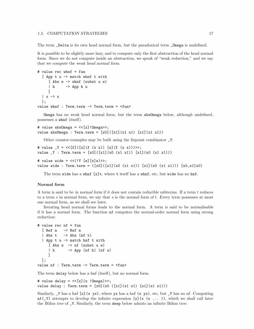
The term _Delta is its own head normal form, but the paradoxical term _Omega is undefined.
It is possible to be slightly more lazy, and to compute only the first abstraction of the head normalform. Since we do not compute inside an abstraction, we speak of “weak reduction,” and we saythat we compute the weak head normal form.
# value rec whnf = fun
[ App t u -> match whnf t with
[ Abs w -> whnf (subst u w)
| h -> App h u
]
| x -> x
];
value whnf : Term.term -> Term.term = <fun>
Omega has no weak head normal form, but the term absOmega below, although undefined,possesses a whnf (itself).
# value absOmega = <<[x]!Omega>>;
value absOmega : Term.term = [x0]([x1](x1 x1) [x1](x1 x1))
Other counter-examples may be built using the fixpoint combinator _Y:
# value _Y = <<[f]([x](f (x x)) [x](f (x x)))>>;
value _Y : Term.term = [x0]([x1](x0 (x1 x1)) [x1](x0 (x1 x1)))
# value wide = <<(!Y [e][x]e)>>;
value wide : Term.term = ([x0]([x1](x0 (x1 x1)) [x1](x0 (x1 x1))) [x0,x1]x0)
The term wide has a whnf [x]t, where t itself has a whnf, etc, but wide has no hnf.
Normal form
A term is said to be in normal form if it does not contain reducible subterms. If a term t reducesto a term s in normal form, we say that s is the normal form of t. Every term possesses at mostone normal form, as we shall see later.
Iterating head normal forms leads to the normal form. A term is said to be normalisableif it has a normal form. The function nf computes the normal-order normal form using strongreduction:
# value rec nf = fun
[ Ref n -> Ref n
| Abs t -> Abs (nf t)
| App t u -> match hnf t with
[ Abs w -> nf (subst u w)
| h -> App (nf h) (nf u)
]
];
value nf : Term.term -> Term.term = <fun>
The term delay below has a hnf (itself), but no normal form.
# value delay = <<[x](x !Omega)>>;
value delay : Term.term = [x0](x0 ([x1](x1 x1) [x1](x1 x1)))
Similarly, _Y has a hnf [x](x yx), where yx has a hnf (x yx), etc, but _Y has no nf. Computingnf(_Y) attempts to develop the infinite expression [x](x (x ... )), which we shall call laterthe Bohm tree of _Y. Similarly, the term deep below admits an infinite Bohm tree:
18 CHAPTER 1. λ-CALCULUS: SYNTAX AND COMPUTATION STRATEGIES
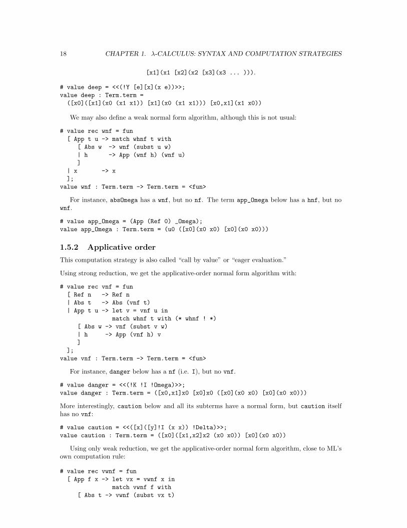
[x1](x1 [x2](x2 [x3](x3 ... ))).
# value deep = <<(!Y [e][x](x e))>>;
value deep : Term.term =
([x0]([x1](x0 (x1 x1)) [x1](x0 (x1 x1))) [x0,x1](x1 x0))
We may also define a weak normal form algorithm, although this is not usual:
# value rec wnf = fun
[ App t u -> match whnf t with
[ Abs w -> wnf (subst u w)
| h -> App (wnf h) (wnf u)
]
| x -> x
];
value wnf : Term.term -> Term.term = <fun>
For instance, absOmega has a wnf, but no nf. The term app_Omega below has a hnf, but nownf.
# value app_Omega = (App (Ref 0) _Omega);
value app_Omega : Term.term = (u0 ([x0](x0 x0) [x0](x0 x0)))
1.5.2 Applicative order
This computation strategy is also called “call by value” or “eager evaluation.”
Using strong reduction, we get the applicative-order normal form algorithm with:
# value rec vnf = fun
[ Ref n -> Ref n
| Abs t -> Abs (vnf t)
| App t u -> let v = vnf u in
match whnf t with (* whnf ! *)
[ Abs w -> vnf (subst v w)
| h -> App (vnf h) v
]
];
value vnf : Term.term -> Term.term = <fun>
For instance, danger below has a nf (i.e. I), but no vnf.
# value danger = <<(!K !I !Omega)>>;
value danger : Term.term = ([x0,x1]x0 [x0]x0 ([x0](x0 x0) [x0](x0 x0)))
More interestingly, caution below and all its subterms have a normal form, but caution itselfhas no vnf:
# value caution = <<([x]([y]!I (x x)) !Delta)>>;
value caution : Term.term = ([x0]([x1,x2]x2 (x0 x0)) [x0](x0 x0))
Using only weak reduction, we get the applicative-order normal form algorithm, close to ML’sown computation rule:
# value rec vwnf = fun
[ App f x -> let vx = vwnf x in
match vwnf f with
[ Abs t -> vwnf (subst vx t)
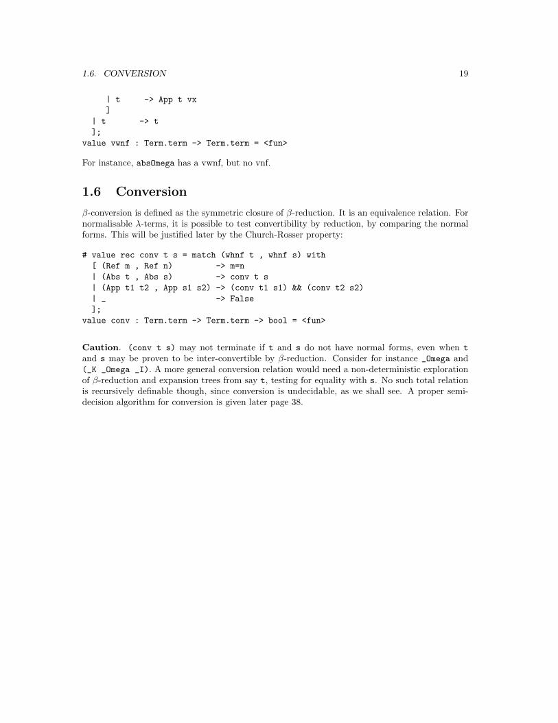
1.6. CONVERSION 19
| t -> App t vx
]
| t -> t
];
value vwnf : Term.term -> Term.term = <fun>
For instance, absOmega has a vwnf, but no vnf.
1.6 Conversion
β-conversion is defined as the symmetric closure of β-reduction. It is an equivalence relation. Fornormalisable λ-terms, it is possible to test convertibility by reduction, by comparing the normalforms. This will be justified later by the Church-Rosser property:
# value rec conv t s = match (whnf t , whnf s) with
[ (Ref m , Ref n) -> m=n
| (Abs t , Abs s) -> conv t s
| (App t1 t2 , App s1 s2) -> (conv t1 s1) && (conv t2 s2)
| _ -> False
];
value conv : Term.term -> Term.term -> bool = <fun>
Caution. (conv t s) may not terminate if t and s do not have normal forms, even when t
and s may be proven to be inter-convertible by β-reduction. Consider for instance _Omega and(_K _Omega _I). A more general conversion relation would need a non-deterministic explorationof β-reduction and expansion trees from say t, testing for equality with s. No such total relationis recursively definable though, since conversion is undecidable, as we shall see. A proper semi-decision algorithm for conversion is given later page 38.

20 CHAPTER 1. λ-CALCULUS: SYNTAX AND COMPUTATION STRATEGIES
Chapter 2
Computability theory based onλ-calculus
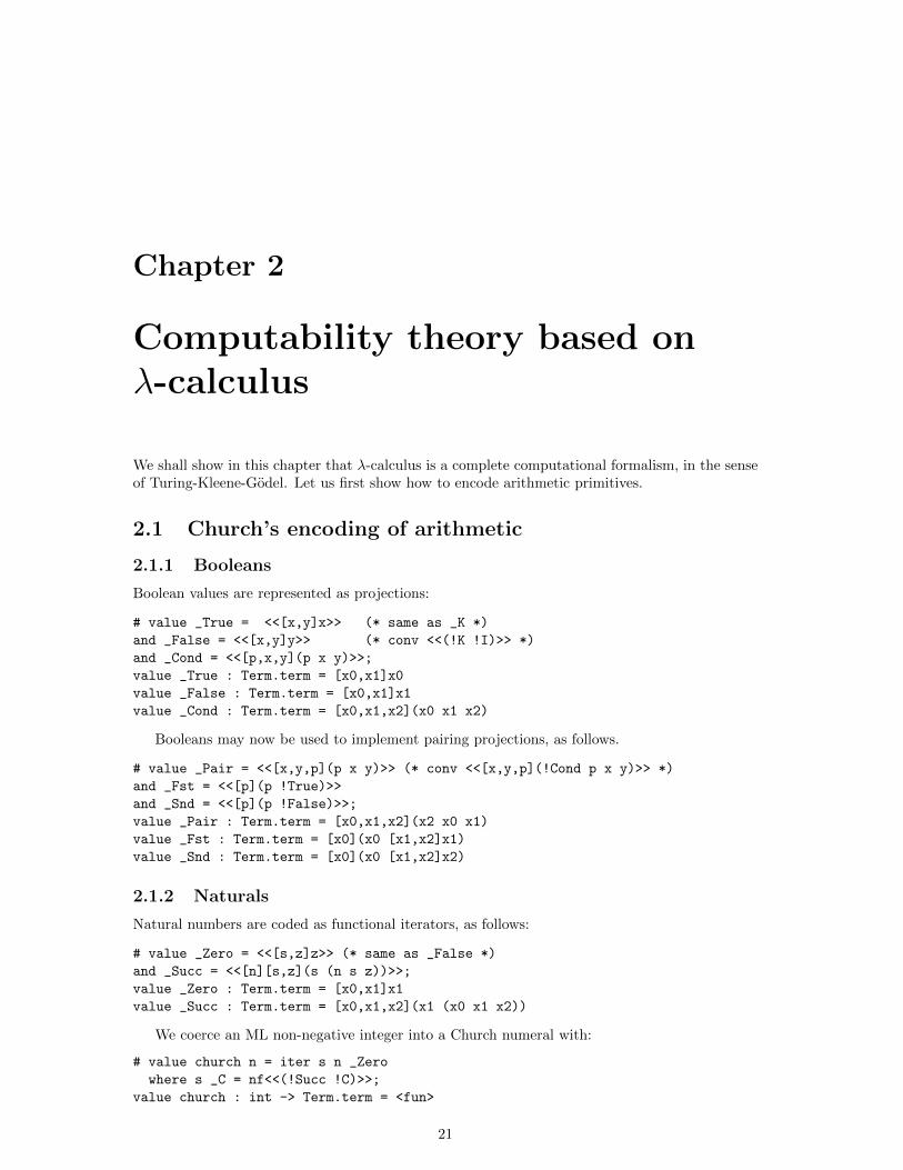
We shall show in this chapter that λ-calculus is a complete computational formalism, in the senseof Turing-Kleene-Godel. Let us first show how to encode arithmetic primitives.
2.1 Church’s encoding of arithmetic
2.1.1 Booleans
Boolean values are represented as projections:
# value _True = <<[x,y]x>> (* same as _K *)
and _False = <<[x,y]y>> (* conv <<(!K !I)>> *)
and _Cond = <<[p,x,y](p x y)>>;
value _True : Term.term = [x0,x1]x0
value _False : Term.term = [x0,x1]x1
value _Cond : Term.term = [x0,x1,x2](x0 x1 x2)
Booleans may now be used to implement pairing projections, as follows.
# value _Pair = <<[x,y,p](p x y)>> (* conv <<[x,y,p](!Cond p x y)>> *)
and _Fst = <<[p](p !True)>>
and _Snd = <<[p](p !False)>>;
value _Pair : Term.term = [x0,x1,x2](x2 x0 x1)
value _Fst : Term.term = [x0](x0 [x1,x2]x1)
value _Snd : Term.term = [x0](x0 [x1,x2]x2)
2.1.2 Naturals
Natural numbers are coded as functional iterators, as follows:
# value _Zero = <<[s,z]z>> (* same as _False *)
and _Succ = <<[n][s,z](s (n s z))>>;
value _Zero : Term.term = [x0,x1]x1
value _Succ : Term.term = [x0,x1,x2](x1 (x0 x1 x2))
We coerce an ML non-negative integer into a Church numeral with:
# value church n = iter s n _Zero
where s _C = nf<<(!Succ !C)>>;
value church : int -> Term.term = <fun>
21
22 CHAPTER 2. COMPUTABILITY THEORY BASED ON λ-CALCULUS
# value _One = church 1
and _Two = church 2
and _Three = church 3
and _Four = church 4
and _Five = church 5;
value _One : Term.term = [x0,x1](x0 x1)
value _Two : Term.term = [x0,x1](x0 (x0 x1))
value _Three : Term.term = [x0,x1](x0 (x0 (x0 x1)))
value _Four : Term.term = [x0,x1](x0 (x0 (x0 (x0 x1))))
value _Five : Term.term = [x0,x1](x0 (x0 (x0 (x0 (x0 x1)))))
We may for instance use Church’s numerals as “for loops”:
# value eval_nat iter init = fun
[ Abs (Abs t) (* [s,z]t *) -> eval_rec t
where rec eval_rec = fun
[ (* z *) Ref 0 -> init
| (* (s u) *) App (Ref 1) u -> iter (eval_rec u)
| _ -> error "Not a normal church natural"
]
| _ -> error "Not a normal church natural"
];
value eval_nat : (’a -> ’a) -> ’a -> Term.term -> ’a = <fun>
Thus, (eval_nat (church n) f x) is equivalent to ML’s (iter f n x).For instance, here is the coercion from Church’s numerals to unary integers:
# value roman = eval_nat (fun s -> "|" ^ s) "";
value roman : Term.term -> string = <fun>
# roman _Four;
- : string = "||||"
Here is the coercion from λ-terms to ML’s integers:
# value compute_nat = eval_nat succ 0;
value compute_nat : Term.term -> int = <fun>
We may compose compute_nat with a computation strategy to evaluate terms to a normalform:
# value normal_nat n = compute_nat (nf n);
value normal_nat : Term.term -> int = <fun>
2.1.3 Arithmetic operations
We may test to 0 using _Null below:
# value _Null = <<[n](n (!K !False) !True)>>;
value _Null : Term.term = [x0](x0 ([x1,x2]x1 [x1,x2]x2) [x1,x2]x1)
And addition may be represented as functional composition:
# value _Add = <<[m,n][s,z](m s (n s z))>>;
value _Add : Term.term = [x0,x1,x2,x3](x0 x2 (x1 x2 x3))
For instance:
2.1. CHURCH’S ENCODING OF ARITHMETIC 23
# normal_nat<<(!Add !Two !Two)>>;
- : int = 4
Remark. There are many possible encodings of natural numbers in λ-calculus. For a givenencoding, there are many algorithms computing extensionally the same function. For instance,here is another successor algorithm, which normalises its result in applicative order:
# value _Succv = <<[n][s,z](n s (s z))>>;
value _Succv : Term.term = [x0,x1,x2](x0 x1 (x1 x2))
Another addition algorithm may be defined as:
# <<[m,n](m !Succ n)>>;
- : Term.term = [x0,x1](x0 [x2,x3,x4](x3 (x2 x3 x4)) x1)
Other versions are obtained by commuting the roles of m and n. Here is an applicative orderaddition:
# value _Addv = <<[m,n](m !Succv [s,z](n s z))>>;
value _Addv : Term.term =
[x0,x1](x0 [x2,x3,x4](x2 x3 (x3 x4)) [x2,x3](x1 x2 x3))
Multiplication may be simply implemented by composition:
# value _Mult = _B;
value _Mult : Term.term = [x0,x1,x2](x0 (x1 x2))
# normal_nat<<(!Mult !Five !Five)>>;
- : int = 25
Again, many other multiplication algorithms exist, such as <<[m,n](m (!Add n) !Zero)>>.
Exponentiation may be defined as the transposed of application:
# value _Exp = <<[m,n](n m)>>;
value _Exp : Term.term = [x0,x1](x1 x0)
# normal_nat<<(!Exp !Three !Five)>>;
- : int = 243
And again, other exponentiation algorithms exist, such as <<[m,n](n (!Mult m) !One)>>.
2.1.4 Primitive recursion
More generally, we may program primitive recursive algorithms using natural numbers as “forloops”. For instance, we compute the factorial function by iterating the computation of the pair(n, factn):
# value _Fact = <<let loop = [p] let n = (!Succ (!Fst p))
in (!Pair n (!Mult n (!Snd p)))
in [n](!Snd (n loop (!Pair !Zero !One)))>>;
value _Fact : Term.term = ([x0,x1]([x2](x2 [x3,x4]x4) (x1 x0 ([x2,x3,x4]
(x4 x2 x3) [x2,x3]x3 [x2,x3](x2 x3)))) [x0]([x1]([x2,x3,x4] (x4 x2 x3)
x1 ([x2,x3,x4](x2 (x3 x4)) x1 ([x2](x2 [x3,x4]x4) x0))) ([x1,x2,x3]
(x2 (x1 x2 x3)) ([x1](x1 [x2,x3]x2) x0))))
# normal_nat<<(!Fact !Five)>>;
- : int = 120
24 CHAPTER 2. COMPUTABILITY THEORY BASED ON λ-CALCULUS
Similarly for the Fibonacci function:
# value _Fib = <<let loop = [p] let fib1 = (!Fst p)
in (!Pair (!Add fib1 (!Snd p)) fib1)
in [n](!Snd (n loop (!Pair !One !One)))>>;
value _Fib : Term.term = ...
Actually, the same idea may be used to compute the predecessor function, in the manner ofKleene:
value _Pred = <<let loop = [p] let pred = (!Fst p)
in (!Pair (!Succ pred) pred)
in [n](!Snd (n loop (!Pair !Zero !Zero)))>>;
From which we get arithmetic comparison:
# value _Geq = <<[m,n](m !Pred n (!K !False) !True)>>;
value _Geq : Term.term = ...
2.1.5 Functional iteration
Actually, iteration is stronger than primitive recursion if we iterate functional values. We may thusgo up the full type hierarchy, defining general arithmetical functions, like in Godel’s DialecticaSystem T.
For instance, let us define functional iteration as follows.
# value _Iter = <<[f][n](n f (f !One))>>;
value _Iter : Term.term = [x0,x1](x1 x0 (x0 [x2,x3](x2 x3)))
We now recall the definition of Ackermann’s function, the typical arithmetical function whichis not primitive recursive, that is not computable with for loops but needs full recursion:
# value ackermann n = ack2(n,n)
where rec ack2 = fun
[ (0,n) -> n+1
| (m,0) -> ack2(m-1,1)
| (m,n) -> ack2(m-1,ack2(m,n-1))
];
value ackermann : int -> int = <fun>
It is easy to define it as a λ-term with the _Iter functional above, as follows:
# value _Ack = <<[n](n !Iter !Succ n)>>;
value _Ack : Term.term =
[x0](x0 [x1,x2](x2 x1 (x1 [x3,x4](x3 x4))) [x1,x2,x3](x2 (x1 x2 x3)) x0)
# normal_nat<<(!Ack !Two)>>;
- : int = 7
This example shows that iteration is more powerful than primitive recursion. More precisely,primitive recursion limits iteration to sequences of integers, and cannot capture functional iter-ations such as _Iter above. Using such functional iteration scheme, every functional of Godel’ssystem T is definable, and thus we may find algorithms for all the number-theoretic functionswhich are provably total in Peano’s arithmetic.
Beware. This does not mean that we may define easily every given algorithm. For instance,the usual algorithm which returns the minimum value of two natural numbers by testing eachinteger in turn is not definable in primitive recursive arithmetic, although it computes a primitiverecursive function (Colson).
2.2. λ-CALCULUS AS A GENERAL PROGRAMMING LANGUAGE 25
2.1.6 General recursion
All the examples given so far are total recursive functions, dealing with normalisable λ-terms. Wenow enter the realm of partial recursive functions and functionals.
We recall the definition of the _Y combinator above:
_Y = <<[f]([x](f (x x)) [x](f (x x)))>>.
_Y is called Curry’s fixpoint combinator. It is a fixpoint in the sense that
conv <<(!Y !F)>> <<(!F (!Y !F))>>
for every λ-term _F. Another fixpoint functional, _Fix, due to Turing, has the further propertythat <<(!Fix !F)>> reduces to <<(!F (!Fix !F))>> in normal order:
# value _Fix = <<([x,f](f (x x f)) [x,f](f (x x f)))>>;
value _Fix : Term.term = ([x0,x1](x1 (x0 x0 x1)) [x0,x1](x1 (x0 x0 x1)))
For instance, the usual recursive definition of the factorial function in ML:value rec fact n = if n=0 then 1 else n*(fact(n-1));
may be directly transcribed in λ-calculus as:
# value _Fact_rec =
<<(!Fix [fact][n](!Cond (!Null n) !One (!Mult n (fact (!Pred n)))))>>;
value _Fact_rec : Term.term = ...
2.1.7 Turing completeness
The above examples should convince the reader that λ-calculus is strong enough a formalism todefine all computable functions. Indeed:
Theorem. Turing completeness of λ-calculus.Every partial recursive function f of k arguments may be represented as a λ-term _F which isextensionally equal to f , in the sense that for all naturals n1, . . . nk, f(n1, . . . , nk) is defined andequal to n if and only if <<(!F !N1 ... !Nk)>> has a normal form, where _Ni = church ni, inwhich case it is equal to church n.
This theorem shows that λ-calculus is a Turing-complete programming language, in which allpartial recursive functions are definable. The negative consequence of this positive fact is thatmany properties of λ-calculus computations become undecidable, as we shall see later.
We shall not bother to prove this theorem, and rather take the point of view that the com-putable functions are exactly the ones that are definable in λ-calculus. Here computable functionscomprise all the standard (partial recursive) arithmetic functions, but we may also define algo-rithms computing over more general data types, without resorting to arithmetic encodings, as weshall see in the next section.
Remark. We may refine the theorem above by requiring the term _F to be in normal formwhenever f is a total function. Note that this last fact is not obvious from the examples above,since for instance _Fact_rec has no normal form. What ML actually computes when given therecursive definition of fact is the vwnf <<[n](!Fact_rec n)>>.
2.2 λ-calculus as a general programming language
We have limited our computations so far to booleans, integers, and pairs. Actually, more generalcomputations on arbitrary recursively defined data types are possible. The general scheme willbe explained in the second part of these notes, when we shall develop these notions inside typetheory. We just give here the special case of list structures.
26 CHAPTER 2. COMPUTABILITY THEORY BASED ON λ-CALCULUS
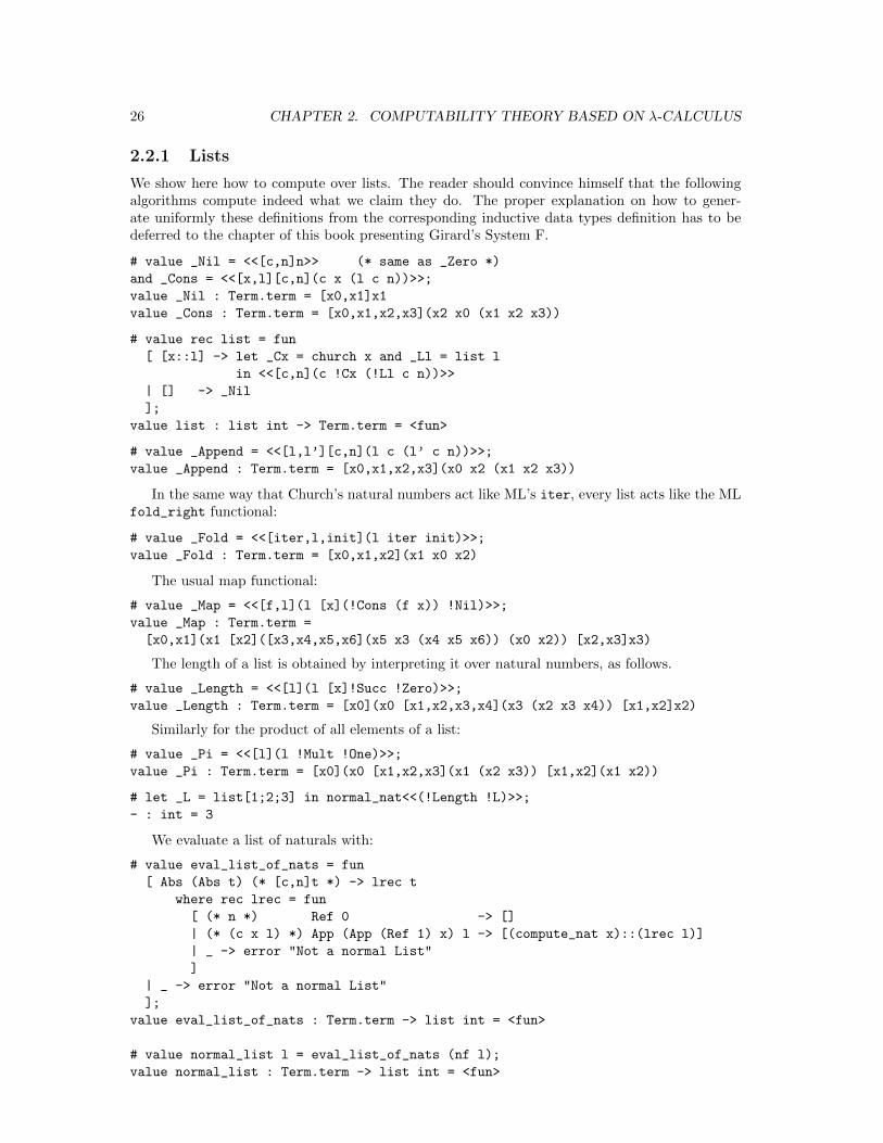
2.2.1 Lists
We show here how to compute over lists. The reader should convince himself that the followingalgorithms compute indeed what we claim they do. The proper explanation on how to gener-ate uniformly these definitions from the corresponding inductive data types definition has to bedeferred to the chapter of this book presenting Girard’s System F.
# value _Nil = <<[c,n]n>> (* same as _Zero *)
and _Cons = <<[x,l][c,n](c x (l c n))>>;
value _Nil : Term.term = [x0,x1]x1
value _Cons : Term.term = [x0,x1,x2,x3](x2 x0 (x1 x2 x3))
# value rec list = fun
[ [x::l] -> let _Cx = church x and _Ll = list l
in <<[c,n](c !Cx (!Ll c n))>>
| [] -> _Nil
];
value list : list int -> Term.term = <fun>
# value _Append = <<[l,l’][c,n](l c (l’ c n))>>;
value _Append : Term.term = [x0,x1,x2,x3](x0 x2 (x1 x2 x3))
In the same way that Church’s natural numbers act like ML’s iter, every list acts like the MLfold_right functional:
# value _Fold = <<[iter,l,init](l iter init)>>;
value _Fold : Term.term = [x0,x1,x2](x1 x0 x2)
The usual map functional:
# value _Map = <<[f,l](l [x](!Cons (f x)) !Nil)>>;
value _Map : Term.term =
[x0,x1](x1 [x2]([x3,x4,x5,x6](x5 x3 (x4 x5 x6)) (x0 x2)) [x2,x3]x3)
The length of a list is obtained by interpreting it over natural numbers, as follows.
# value _Length = <<[l](l [x]!Succ !Zero)>>;
value _Length : Term.term = [x0](x0 [x1,x2,x3,x4](x3 (x2 x3 x4)) [x1,x2]x2)
Similarly for the product of all elements of a list:
# value _Pi = <<[l](l !Mult !One)>>;
value _Pi : Term.term = [x0](x0 [x1,x2,x3](x1 (x2 x3)) [x1,x2](x1 x2))
# let _L = list[1;2;3] in normal_nat<<(!Length !L)>>;
- : int = 3
We evaluate a list of naturals with:
# value eval_list_of_nats = fun
[ Abs (Abs t) (* [c,n]t *) -> lrec t
where rec lrec = fun
[ (* n *) Ref 0 -> []
| (* (c x l) *) App (App (Ref 1) x) l -> [(compute_nat x)::(lrec l)]
| _ -> error "Not a normal List"
]
| _ -> error "Not a normal List"
];
value eval_list_of_nats : Term.term -> list int = <fun>
# value normal_list l = eval_list_of_nats (nf l);
value normal_list : Term.term -> list int = <fun>
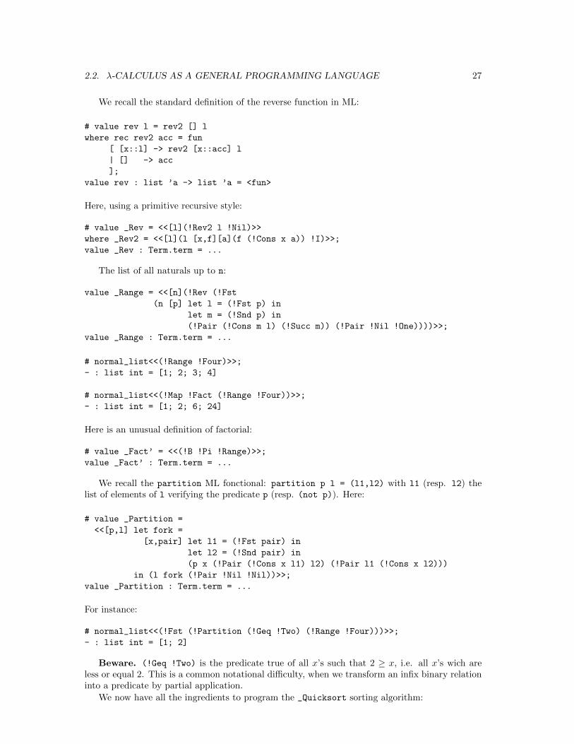
2.2. λ-CALCULUS AS A GENERAL PROGRAMMING LANGUAGE 27
We recall the standard definition of the reverse function in ML:
# value rev l = rev2 [] l
where rec rev2 acc = fun
[ [x::l] -> rev2 [x::acc] l
| [] -> acc
];
value rev : list ’a -> list ’a = <fun>
Here, using a primitive recursive style:
# value _Rev = <<[l](!Rev2 l !Nil)>>
where _Rev2 = <<[l](l [x,f][a](f (!Cons x a)) !I)>>;
value _Rev : Term.term = ...
The list of all naturals up to n:
value _Range = <<[n](!Rev (!Fst
(n [p] let l = (!Fst p) in
let m = (!Snd p) in
(!Pair (!Cons m l) (!Succ m)) (!Pair !Nil !One))))>>;
value _Range : Term.term = ...
# normal_list<<(!Range !Four)>>;
- : list int = [1; 2; 3; 4]
# normal_list<<(!Map !Fact (!Range !Four))>>;
- : list int = [1; 2; 6; 24]
Here is an unusual definition of factorial:
# value _Fact’ = <<(!B !Pi !Range)>>;
value _Fact’ : Term.term = ...
We recall the partition ML fonctional: partition p l = (l1,l2) with l1 (resp. l2) thelist of elements of l verifying the predicate p (resp. (not p)). Here:
# value _Partition =
<<[p,l] let fork =
[x,pair] let l1 = (!Fst pair) in
let l2 = (!Snd pair) in
(p x (!Pair (!Cons x l1) l2) (!Pair l1 (!Cons x l2)))
in (l fork (!Pair !Nil !Nil))>>;
value _Partition : Term.term = ...
For instance:
# normal_list<<(!Fst (!Partition (!Geq !Two) (!Range !Four)))>>;
- : list int = [1; 2]
Beware. (!Geq !Two) is the predicate true of all x’s such that 2 ≥ x, i.e. all x’s wich areless or equal 2. This is a common notational difficulty, when we transform an infix binary relationinto a predicate by partial application.
We now have all the ingredients to program the _Quicksort sorting algorithm:
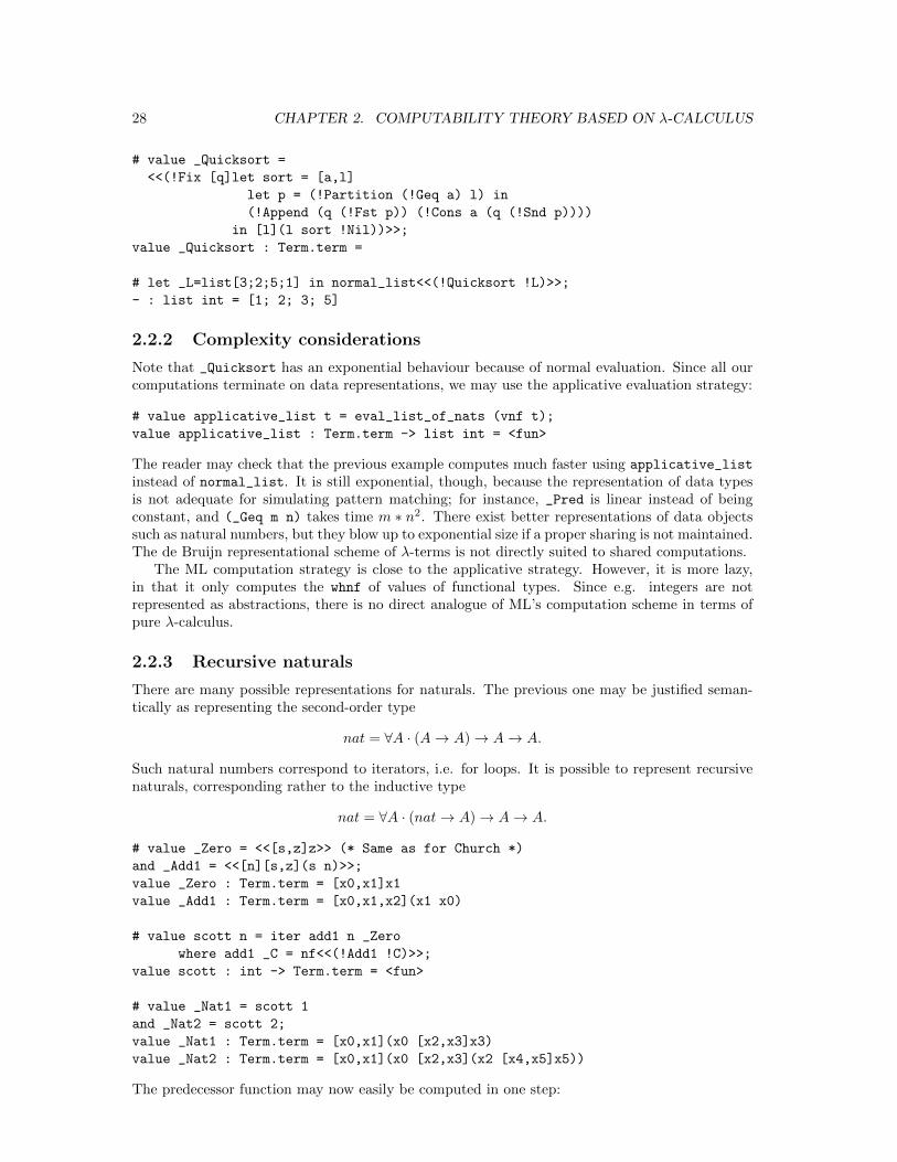
28 CHAPTER 2. COMPUTABILITY THEORY BASED ON λ-CALCULUS
# value _Quicksort =
<<(!Fix [q]let sort = [a,l]
let p = (!Partition (!Geq a) l) in
(!Append (q (!Fst p)) (!Cons a (q (!Snd p))))
in [l](l sort !Nil))>>;
value _Quicksort : Term.term =
# let _L=list[3;2;5;1] in normal_list<<(!Quicksort !L)>>;
- : list int = [1; 2; 3; 5]
2.2.2 Complexity considerations
Note that _Quicksort has an exponential behaviour because of normal evaluation. Since all ourcomputations terminate on data representations, we may use the applicative evaluation strategy:
# value applicative_list t = eval_list_of_nats (vnf t);
value applicative_list : Term.term -> list int = <fun>
The reader may check that the previous example computes much faster using applicative_list
instead of normal_list. It is still exponential, though, because the representation of data typesis not adequate for simulating pattern matching; for instance, _Pred is linear instead of beingconstant, and (_Geq m n) takes time m ∗ n2. There exist better representations of data objectssuch as natural numbers, but they blow up to exponential size if a proper sharing is not maintained.The de Bruijn representational scheme of λ-terms is not directly suited to shared computations.
The ML computation strategy is close to the applicative strategy. However, it is more lazy,in that it only computes the whnf of values of functional types. Since e.g. integers are notrepresented as abstractions, there is no direct analogue of ML’s computation scheme in terms ofpure λ-calculus.
2.2.3 Recursive naturals
There are many possible representations for naturals. The previous one may be justified seman-tically as representing the second-order type
nat = ∀A · (A→ A)→ A→ A.
Such natural numbers correspond to iterators, i.e. for loops. It is possible to represent recursivenaturals, corresponding rather to the inductive type
nat = ∀A · (nat→ A)→ A→ A.
# value _Zero = <<[s,z]z>> (* Same as for Church *)
and _Add1 = <<[n][s,z](s n)>>;
value _Zero : Term.term = [x0,x1]x1
value _Add1 : Term.term = [x0,x1,x2](x1 x0)
# value scott n = iter add1 n _Zero
where add1 _C = nf<<(!Add1 !C)>>;
value scott : int -> Term.term = <fun>
# value _Nat1 = scott 1
and _Nat2 = scott 2;
value _Nat1 : Term.term = [x0,x1](x0 [x2,x3]x3)
value _Nat2 : Term.term = [x0,x1](x0 [x2,x3](x2 [x4,x5]x5))
The predecessor function may now easily be computed in one step:
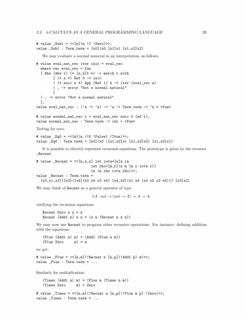
2.2. λ-CALCULUS AS A GENERAL PROGRAMMING LANGUAGE 29
# value _Sub1 = <<[n](n !I !Zero)>>;
value _Sub1 : Term.term = [x0](x0 [x1]x1 [x1,x2]x2)
We may evaluate a normal numeral in an interpetation, as follows.
# value eval_nat_rec iter init = eval_rec
where rec eval_rec = fun
[ Abs (Abs t) (* [s,z]t *) -> match t with
[ (* z *) Ref 0 -> init
| (* succ s *) App (Ref 1) s -> iter (eval_rec s)
| _ -> error "Not a normal natural"
]
| _ -> error "Not a normal natural"
];
value eval_nat_rec : (’a -> ’a) -> ’a -> Term.term -> ’a = <fun>
# value normal_nat_rec t = eval_nat_rec succ 0 (nf t);
value normal_nat_rec : Term.term -> int = <fun>
Testing for zero:
# value _Eq0 = <<[n](n (!K !False) !True)>>;
value _Eq0 : Term.term = [x0](x0 ([x1,x2]x1 [x1,x2]x2) [x1,x2]x1)
It is possible to directly represent recursion equations. The prototype is given by the recursor_Recnat:
# value _Recnat = <<[n,s,z] let iota=[x]z in
let rho=[m,r](s m (m r iota r))
in (n rho iota rho)>>;
value _Recnat : Term.term =
[x0,x1,x2]([x3]([x4](x0 x4 x3 x4) [x4,x5](x1 x4 (x4 x5 x3 x5))) [x3]x2)
We may think of Recnat as a general operator of type
∀A · nat→ (nat→ A)→ A→ A,
verifying the recursion equations:
Recnat Zero s z = z
Recnat (Add1 n) s z = (s n (Recnat n s z))
We may now use Recnat to program other recursive operations. For instance, defining additionwith the equations:
(Plus (Add1 n) m) = (Add1 (Plus n m))
(Plus Zero m) = m
we get:
# value _Plus = <<[n,m](!Recnat n [n,p](!Add1 p) m)>>;
value _Plus : Term.term = ...
Similarly for multiplication:
(Times (Add1 n) m) = (Plus m (Times n m))
(Times Zero m) = Zero
# value _Times = <<[n,m](!Recnat n [n,p](!Plus m p) !Zero)>>;
value _Times : Term.term = ...
30 CHAPTER 2. COMPUTABILITY THEORY BASED ON λ-CALCULUS
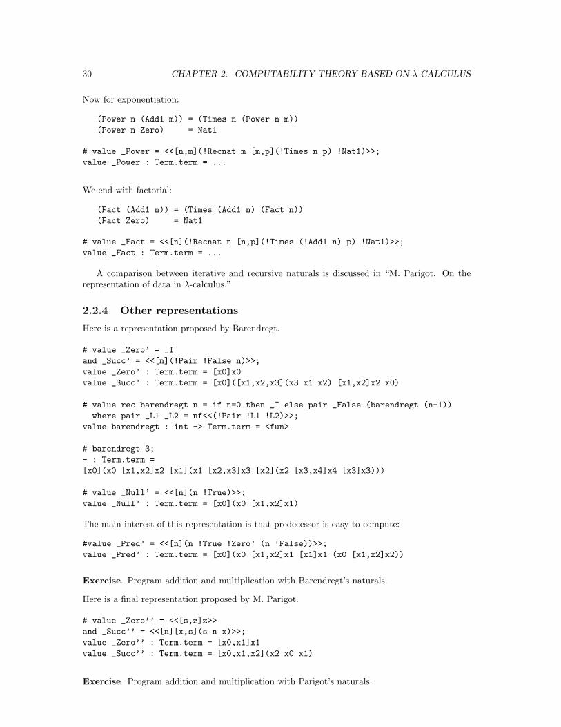
Now for exponentiation:
(Power n (Add1 m)) = (Times n (Power n m))
(Power n Zero) = Nat1
# value _Power = <<[n,m](!Recnat m [m,p](!Times n p) !Nat1)>>;
value _Power : Term.term = ...
We end with factorial:
(Fact (Add1 n)) = (Times (Add1 n) (Fact n))
(Fact Zero) = Nat1
# value _Fact = <<[n](!Recnat n [n,p](!Times (!Add1 n) p) !Nat1)>>;
value _Fact : Term.term = ...
A comparison between iterative and recursive naturals is discussed in “M. Parigot. On therepresentation of data in λ-calculus.”
2.2.4 Other representations
Here is a representation proposed by Barendregt.
# value _Zero’ = _I
and _Succ’ = <<[n](!Pair !False n)>>;
value _Zero’ : Term.term = [x0]x0
value _Succ’ : Term.term = [x0]([x1,x2,x3](x3 x1 x2) [x1,x2]x2 x0)
# value rec barendregt n = if n=0 then _I else pair _False (barendregt (n-1))
where pair _L1 _L2 = nf<<(!Pair !L1 !L2)>>;
value barendregt : int -> Term.term = <fun>
# barendregt 3;
- : Term.term =
[x0](x0 [x1,x2]x2 [x1](x1 [x2,x3]x3 [x2](x2 [x3,x4]x4 [x3]x3)))
# value _Null’ = <<[n](n !True)>>;
value _Null’ : Term.term = [x0](x0 [x1,x2]x1)
The main interest of this representation is that predecessor is easy to compute:
#value _Pred’ = <<[n](n !True !Zero’ (n !False))>>;
value _Pred’ : Term.term = [x0](x0 [x1,x2]x1 [x1]x1 (x0 [x1,x2]x2))
Exercise. Program addition and multiplication with Barendregt’s naturals.
Here is a final representation proposed by M. Parigot.
# value _Zero’’ = <<[s,z]z>>
and _Succ’’ = <<[n][x,s](s n x)>>;
value _Zero’’ : Term.term = [x0,x1]x1
value _Succ’’ : Term.term = [x0,x1,x2](x2 x0 x1)
Exercise. Program addition and multiplication with Parigot’s naturals.
2.3. RUDIMENTS OF RECURSION THEORY 31
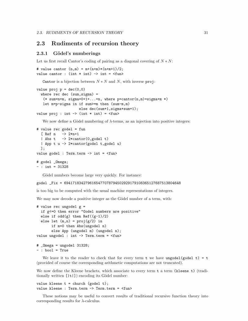
2.3 Rudiments of recursion theory
2.3.1 Godel’s numberings
Let us first recall Cantor’s coding of pairing as a diagonal covering of N ∗N :
# value cantor (n,m) = m+(n+m)*(n+m+1)/2;
value cantor : (int * int) -> int = <fun>
Cantor is a bijection between N ∗N and N , with inverse proj:
value proj p = dec(0,0)
where rec dec (sum,sigma) =
(* sum=n+m, sigma=0+1+...+n, where p=cantor(n,m)=sigma+m *)
let m=p-sigma in if sum>=m then (sum-m,m)
else dec(sum+1,sigma+sum+1);
value proj : int -> (int * int) = <fun>
We now define a Godel numbering of λ-terms, as an injection into positive integers:
# value rec godel = fun
[ Ref n -> 2*n+1
| Abs t -> 2*cantor(0,godel t)
| App t u -> 2*cantor(godel t,godel u)
];
value godel : Term.term -> int = <fun>
# godel _Omega;
- : int = 31328
Godel numbers become large very quickly. For instance:
godel _Fix = 6941718342796165477078794502929179108365127687513804648
is too big to be computed with the usual machine representations of integers.
We may now decode a positive integer as the Godel number of a term, with:
# value rec ungodel g =
if g<=0 then error "Godel numbers are positive"
else if odd(g) then Ref((g-1)/2)
else let (m,n) = proj(g/2) in
if m=0 then Abs(ungodel n)
else App (ungodel m) (ungodel n);
value ungodel : int -> Term.term = <fun>
# _Omega = ungodel 31328;
- : bool = True
We leave it to the reader to check that for every term t we have ungodel(godel t) = t
(provided of course the corresponding arithmetic computations are not truncated).
We now define the Kleene brackets, which associate to every term t a term (kleene t) (tradi-tionally written [|t|]) encoding its Godel number:
value kleene t = church (godel t);
value kleene : Term.term -> Term.term = <fun>
These notions may be useful to convert results of traditional recursive function theory intocorresponding results for λ-calculus.
32 CHAPTER 2. COMPUTABILITY THEORY BASED ON λ-CALCULUS
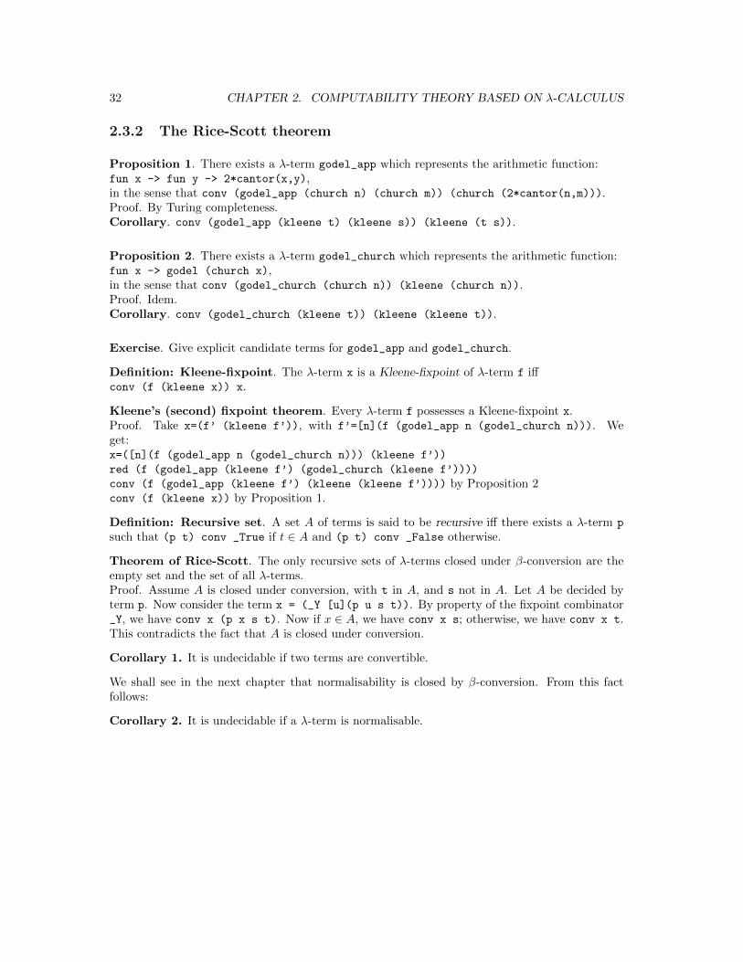
2.3.2 The Rice-Scott theorem
Proposition 1. There exists a λ-term godel_app which represents the arithmetic function:fun x -> fun y -> 2*cantor(x,y),in the sense that conv (godel_app (church n) (church m)) (church (2*cantor(n,m))).Proof. By Turing completeness.Corollary. conv (godel_app (kleene t) (kleene s)) (kleene (t s)).
Proposition 2. There exists a λ-term godel_church which represents the arithmetic function:fun x -> godel (church x),in the sense that conv (godel_church (church n)) (kleene (church n)).Proof. Idem.Corollary. conv (godel_church (kleene t)) (kleene (kleene t)).
Exercise. Give explicit candidate terms for godel_app and godel_church.
Definition: Kleene-fixpoint. The λ-term x is a Kleene-fixpoint of λ-term f iffconv (f (kleene x)) x.
Kleene’s (second) fixpoint theorem. Every λ-term f possesses a Kleene-fixpoint x.Proof. Take x=(f’ (kleene f’)), with f’=[n](f (godel_app n (godel_church n))). Weget:x=([n](f (godel_app n (godel_church n))) (kleene f’))
red (f (godel_app (kleene f’) (godel_church (kleene f’))))
conv (f (godel_app (kleene f’) (kleene (kleene f’)))) by Proposition 2conv (f (kleene x)) by Proposition 1.
Definition: Recursive set. A set A of terms is said to be recursive iff there exists a λ-term p
such that (p t) conv _True if t ∈ A and (p t) conv _False otherwise.
Theorem of Rice-Scott. The only recursive sets of λ-terms closed under β-conversion are theempty set and the set of all λ-terms.Proof. Assume A is closed under conversion, with t in A, and s not in A. Let A be decided byterm p. Now consider the term x = (_Y [u](p u s t)). By property of the fixpoint combinator_Y, we have conv x (p x s t). Now if x ∈ A, we have conv x s; otherwise, we have conv x t.This contradicts the fact that A is closed under conversion.
Corollary 1. It is undecidable if two terms are convertible.
We shall see in the next chapter that normalisability is closed by β-conversion. From this factfollows:
Corollary 2. It is undecidable if a λ-term is normalisable.
Chapter 3
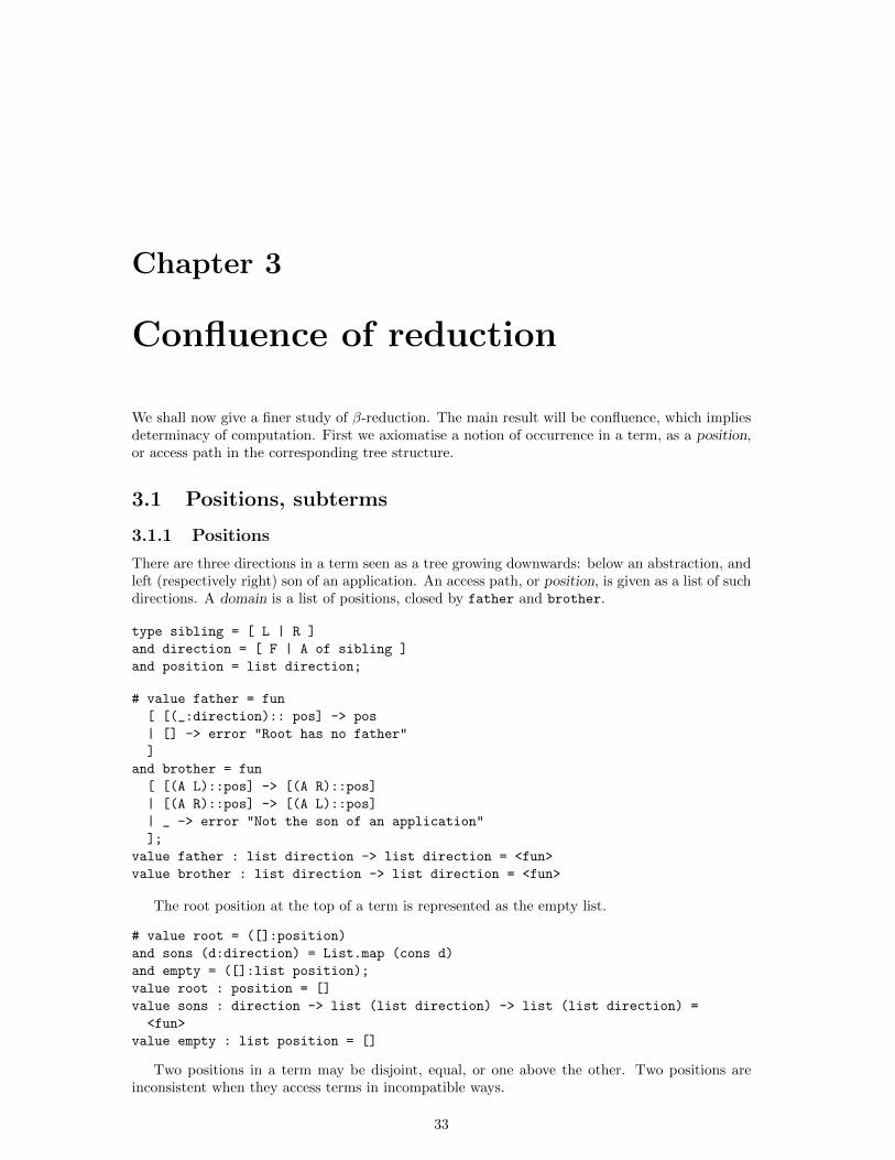
Confluence of reduction
We shall now give a finer study of β-reduction. The main result will be confluence, which impliesdeterminacy of computation. First we axiomatise a notion of occurrence in a term, as a position,or access path in the corresponding tree structure.
3.1 Positions, subterms
3.1.1 Positions
There are three directions in a term seen as a tree growing downwards: below an abstraction, andleft (respectively right) son of an application. An access path, or position, is given as a list of suchdirections. A domain is a list of positions, closed by father and brother.
type sibling = [ L | R ]
and direction = [ F | A of sibling ]
and position = list direction;
# value father = fun
[ [(_:direction):: pos] -> pos
| [] -> error "Root has no father"
]
and brother = fun
[ [(A L)::pos] -> [(A R)::pos]
| [(A R)::pos] -> [(A L)::pos]
| _ -> error "Not the son of an application"
];
value father : list direction -> list direction = <fun>
value brother : list direction -> list direction = <fun>
The root position at the top of a term is represented as the empty list.
# value root = ([]:position)
and sons (d:direction) = List.map (cons d)
and empty = ([]:list position);
value root : position = []
value sons : direction -> list (list direction) -> list (list direction) =
<fun>
value empty : list position = []
Two positions in a term may be disjoint, equal, or one above the other. Two positions areinconsistent when they access terms in incompatible ways.
33
34 CHAPTER 3. CONFLUENCE OF REDUCTION
type comparison =
[ Eq | Less | Greater | Left | Right | Inconsistent ];
# value rec compare = fun
[ ([],[]) -> Eq
| ([],_) -> Less
| (_,[]) -> Greater
| ([(A s)::u],[(A s’)::v]) -> match (s,s’) with
[ (L,R) -> Left
| (R,L) -> Right
| _ -> compare(u,v)
]
| ([F::u],[F::v]) -> compare(u,v)
| _ -> Inconsistent
];
value compare : (list direction * list direction) -> Reduction.comparison =
<fun>
# value disjoint u v =
let test=compare(u,v) in test=Left || test=Right;
value disjoint : list direction -> list direction -> bool = <fun>
# value outer u v =
let test=compare(u,v) in test=Less || test=Left;
value outer : list direction -> list direction -> bool = <fun>
Position u is above or to the left of position v iff (outer u v). Note that outer is a stricttotal ordering on mutually consistent positions. We compute the maximal commun prefix of twoconsistent positions, with corresponding suffixes, with:
# value factor = fact_prefix root
where rec fact_prefix w = fun
[ ([F::u],[F::v]) -> fact_prefix [F::w] (u,v)
| ([(A s)::u],[(A s’)::v]) -> if s=s’ then fact_prefix [(A s)::w] (u,v)
else (List.rev(w) , ([(A s)::u],[(A s’)::v]))
| ([],v) -> (List.rev(w) , ([],v))
| (u,[]) -> (List.rev(w) , (u,[]))
| _ -> error "Inconsistent positions"
];
value factor : (list direction * list direction) ->
(list direction * (list direction * list direction)) = <fun>
We compute the number of abstractions visited by a position with:
# value transfer = trans 0
where rec trans n = fun
[ [F::u] -> trans (n+1) u
| [_::u] -> trans n u
| [] -> n
];
value transfer : list direction -> int = <fun>
The domain of all positions in a term:
# value rec dom = fun
[ Ref m -> [root]
3.1. POSITIONS, SUBTERMS 35
| Abs e -> [root :: (List.map (cons F) (dom e))]
| App e1 e2 -> [root :: (List.map (cons (A L)) (dom e1))] @
(List.map (cons (A R)) (dom e2))
];
value dom : Term.term -> list position = <fun>
For instance:
# dom<<[x](x [y](x y))>>;
- : list position =
[[]; [F]; [F; A L]; [F; A R]; [F; A R; F]; [F; A R; F; A L]; [F; A R; F; A R]]
3.1.2 Subterms
The subterm of λ-term M at position u is defined as subterm(M,u).
# value rec subterm = fun
[ (e,[]) -> e
| (Abs(e),[F::u]) -> subterm(e,u)
| (App e _,[(A L)::u]) -> subterm(e,u)
| (App _ e,[(A R)::u]) -> subterm(e,u)
| _ -> error "Position not in domain"
];
value subterm : (Term.term * list direction) -> Term.term = <fun>
The equality of two subterms may be defined with the inverse of lifting, as follows.
# exception Occurs_free;
This exception is raised when trying to unlift a non-lifted term.
# value unlift1 = unlift_check 0
where rec unlift_check n = fun
[ Ref i -> if i=n then raise Occurs_free
else if i<n then Ref(i) else Ref(i-1)
| Abs t -> Abs (unlift_check (n+1) t)
| App t u -> App (unlift_check n t) (unlift_check n u)
];
value unlift1 : Term.term -> Term.term = <fun>
Note that (unlift1 (lift 1 t)) = t for every term t.
# value unlift = iter unlift1;
value unlift : int -> Term.term -> Term.term = <fun>
value rec eq_subterm t (u,v) =
let (_,(u’,v’)) = factor(u,v)
and tu = subterm(t,u)
and tv = subterm(t,v)
in try unlift (transfer u’) tu = unlift (transfer v’) tv
with [Occurs_free -> False];
value eq_subterm : Term.term ->
(list Reduction.direction * list Reduction.direction) -> bool = <fun>
The term t, where we replace the subterm at position u by term s, may be computed asreplace s (t,u), with replace defined as follows.
36 CHAPTER 3. CONFLUENCE OF REDUCTION
# value replace w = rep_rec
where rec rep_rec = fun
[ (_,[]) -> w
| (Abs e,[F::u]) -> Abs (rep_rec (e,u))
| (App l r,[(A L)::u]) -> App (rep_rec (l,u)) r
| (App l r,[(A R)::u]) -> App l (rep_rec (r,u))
| _ -> error "Position not in domain"
];
value replace : Term.term ->
(Term.term * list Reduction.direction) -> Term.term = <fun>
3.2 Reduction
3.2.1 Redexes
We may now define precisely “u is a (β) redex position in λ-term t”:
# value is_redex t u = match subterm(t,u) with
[ App (Abs _) _ -> True
| _ -> False
];
value is_redex : Term.term -> list Reduction.direction -> bool = <fun>
All redex positions in a λ-term, in outer order:
# value rec redexes = fun
[ Ref _ -> empty
| Abs e -> sons F (redexes e)
| App (Abs e) d -> [root :: (sons (A L) (sons F (redexes e)))]
@ (sons (A R) (redexes d))
| App g d -> (sons (A L) (redexes g)) @ (sons (A R) (redexes d))
];
value redexes : Term.term -> list Reduction.position = <fun>
Note that redexes t = List.filter (is_redex t) (dom t).A term is in normal form when it has no redexes:
# value is_normal t = (redexes t) = [];
value is_normal : Term.term -> bool = <fun>
3.2.2 β-reduction and conversion
One step of β-reduction of term t at redex position u is obtained by reduce t u:
# value reduce t u = match subterm(t,u) with
[ App (Abs body) arg -> replace (subst arg body) (t,u)
| _ -> error "Position not a redex"
];
value reduce : Term.term -> list Reduction.direction -> Term.term = <fun>
We reduce a sequence of redex positions with:
# value reduce_seq = List.fold_left reduce;
value reduce_seq : Term.term -> list (list Reduction.direction)
-> Term.term = <fun>
3.2. REDUCTION 37
Reduction is the reflexive-transitive closure of β-reduction. Here is first a naive definition ofthis relation.
# value rec red t u = (* depth-first *)
u=t || List.exists (fun w -> red (reduce t w) u) (redexes t);
value red : Term.term -> Term.term -> bool = <fun>
This definition works only for strongly normalisable terms, which do not have infinite reductionsequences. It tries to enumerate reducts of t in a depth-first manner, with redexes chosen in outerorder. A more complete definition dove-tails the reductions in a breadth-first manner, giving asemi-decision algorithm for reduction, as follows. First we define all the one-step reducts of termt (with possible duplicates):
# value reducts1 t = List.map (reduce t) (redexes t);
value reducts1 : Term.term -> list Term.term = <fun>
Now we define correctly red as a semi-decision algorithm. As we saw in the last chapter, reductionbeing undecidable, we cannot do better.
# value red t u = redrec [t] (* breadth-first *)
where rec redrec = fun
[ [] -> False
| [t::l] -> (t=u) || redrec(l @ (reducts1 t))
];
value red : Term.term -> Term.term -> bool = <fun>
For instance:
# red <<(!Omega (!Succ !Zero))>> <<(!Omega !One)>>;
- : bool = True
# red <<(!Fix !K)>> <<(!K (!Fix !K))>>;
- : bool = True
But the evaluation of red <<(!Y !K)>> <<(!K (!Y !K))>> would still loop forever.
The following conversion relation is in the same spirit. It is based on the confluence property ofβ-reduction, which we shall prove later. It enumerates the reductions issued from both terms,looking for a common reduct.
# value common_reduct r1 (t,u) =
let rec convrec1 = fun
[ ([], rm, [], rn) -> False
| ([], rm, qn, rn) -> convrec2([], rm, qn, rn)
| ([m::qm], rm, qn, rn) -> (List.mem m rn)
|| convrec2(qm@(r1 m), [m::rm], qn, rn)
]
and convrec2 = fun
[ (qm, rm, [], rn) -> convrec1(qm, rm, [], rn)
| (qm, rm, [n::qn], rn) -> (List.mem n rm)
|| convrec1(qm, rm, qn@(r1 n), [n::rn])
]
in convrec1 ([t],[],[u],[]);
value common_reduct : (’a -> list ’a) -> (’a * ’a) -> bool = <fun>
# value conv t u = common_reduct reducts1 (t,u);
value conv : Term.term -> Term.term -> bool = <fun>
38 CHAPTER 3. CONFLUENCE OF REDUCTION
This repairs the naive conversion algorithm given in the first chapter. Whenever terms t ands are convertible, (i.e. have a common reduct), conv t s will evaluate to True. When t and s
are not convertible, conv t s may loop; it evaluates to False, when both t and u are stronglynormalizing (all rewrite sequences terminate).
For instance, we now get:
# conv <<(!Y !K)>> <<(!K (!Y !K))>>;
- : bool = True
# conv _Zero _Zero’;
- : bool = False
But conv _Y _Fix loops, and conv <<(!Pred’ (!Succ’ !Zero’))>> _Zero’ evaluates to True
after a very long computation indeed.
3.2.3 Leftmost-outermost strategy
Let us reconsider in more detail the normal strategy of reduction, which proceeds in a leftmost-outermost fashion.
# exception Normal_Form;
# value outermost = search_left root
where rec search_left u = fun
[ Ref _ -> raise Normal_Form
| Abs e -> search_left [F::u] e
| App (Abs _) _ -> List.rev u
| App l r -> try search_left [(A L)::u] l
with [ Normal_Form -> search_left [(A R)::u] r ]
];
value outermost : Term.term -> list Reduction.direction = <fun>
One step of normal strategy is given by:
# value one_step_normal t = reduce t (outermost t);
value one_step_normal : Term.term -> Term.term = <fun>
An equivalent optimised definition is osn below:
# value rec osn = fun
[ Ref n -> raise Normal_Form
| Abs lam -> Abs (osn lam)
| App lam1 lam2 -> match lam1 with
[ Abs lam -> subst lam2 lam
| _ -> try App (osn lam1) lam2
with [ Normal_Form -> App lam1 (osn lam2) ]
]
];
value osn : Term.term -> Term.term = <fun>
And the normal strategy nf given in section 1.5.1 may be seen as an optimisation of:
# value rec normalise t = try normalise (osn t)
with [ Normal_Form -> t ];
value normalise : Term.term -> Term.term = <fun>
Value normalise is <fun> : term -> term
3.2. REDUCTION 39
Thus:
# compute_nat (normalise <<(!Add !Two !Two)>>);
- : int = 4
The normal derivation sequence issued from a term t and leading to its normal form, when itexists, is given by:
# value rec normal_sequence t =
try let u = outermost t in
let s = reduce t u in
[u :: (normal_sequence s)]
with [ Normal_Form -> [] ];
value normal_sequence : Term.term -> list (list Reduction.direction) = <fun>
For instance:
# List.length(normal_sequence <<(!Fact !Three)>>);
- : int = 191
If we generalise to an arbitrary strategy or interpreter, we get a non-deterministic computationrule, the choice of the redex position argument of the reduce function being arbitrary. However, weshall see that the computation is ultimately determinate, in the sense of confluence of β-reduction.
We recall that a relation R is said to be strongly confluent iff for every x, y, z, with x R yand x R z, there exists u such that y R u and z R u. A relation R is said to be confluent iff itsreflexive-transitive closure R∗ is strongly confluent. Finally, we say that R is locally confluent ifffor every x, y, z, with x R y and x R z, there exists u such that y R∗ u and z R∗ u. Newman’slemma states that local confluence implies confluence, for strongly normalising relations, for whichthere is no infinite sequence x1 R x2 R x3 R . . ..
It is fairly easy to prove local confluence of β-reduction, in the form that for any positions u andv in term t, we may get from the two terms (reduce t u) and (reduce t v) to a common one,reducing the sequence of (disjoint) redex positions (residuals t u v) and (residuals t v u)
respectively, with the notion of residuals explained in the next section.
3.2.4 Residuals
We start with a technical definition of all the positions of the most recent free variable in a term.
# value locals = loc 0
where rec loc n = fun
[ Ref m -> if m=n then [root] else []
| Abs t -> List.map (cons F) (loc (n+1) t)
| App t u -> List.map (cons (A L)) (loc n t) @
List.map (cons (A R)) (loc n u)
];
value locals : Term.term -> list Reduction.position = <fun>
Intuitively, the residuals of a position are the positions of all copies of the correspondingsubterm after one step of reduction. More precisely, all residuals of position v in term t after itsreduction at redex position u are given by (residuals t u v). This is a set of positions in theterm (reduce t u).
# value residuals t u =
let x = locals(subterm(t,u@[A(L);F])) in fun v -> res(u,v)
where rec res = fun
[ ([],[]) -> []
| ([],[A L]) -> []
40 CHAPTER 3. CONFLUENCE OF REDUCTION
| ([],[(A L)::[F::w]]) -> if List.mem w x then [] else [u@w]
| ([],[(A R)::w]) -> let splice x = u@x@w in List.map splice x
| ([],_) -> error "Position not in domain"
| (_,[]) -> [v]
| ([F::w],[F::w’]) -> res(w,w’)
| ([(A s)::w],[(A s’)::w’]) -> if s=s’ then res(w,w’) else [v]
| _ -> error "Position not in domain"
];
value residuals : Term.term -> list Reduction.direction ->
list Reduction.direction -> list (list Reduction.direction) = <fun>
We leave as exercise to the reader the proof of the following easy fact.
Proposition. Let s=(reduce t u). If v is a redex position of t, then every position in the term(residuals t u v) is a redex position of s. Furthermore, for each position w of s, there is exactlyone position v of t such that w is in (residuals t u v).
Definition. Let s=reduce t u. We say that v is a residual redex position in s iff v is a positionin s which is a residual of some redex position in t. Other redex positions of s are said to becreated redex positions.
Remark. A redex r=([x]t s) may create by its reductions new redexes in three possible ways.Creations downward occur for every subterm in t of the form (x p), when s is an abstraction.A creation upward occurs when r itself is the immediate left son of an application, and t isan abstraction. Finally, a collapse creation occurs when t=x, s is an abstraction, and r is theimmediate left son of an application.
Exercise. Give examples of all three cases of creation of a redex.
Beware. The positions in (residuals t u v) are mutually disjoint, and the corresponding sub-terms are equal (in the sense of eq_subterm). But these properties are not very important, becausethey are not preserved by reduction, as the example below will demonstrate.
We could at this point proceed with proving local confluence of reduction. However, this will not bedirectly sufficient, since the possible non-termination of reduction does not allow using Newman’slemma to get confluence from local confluence. We must rather prove a strong confluence diagram,(the Diamond Lemma below) for a more general notion of parallel reduction. Confluence of β-reduction will follow from the fact that reduction and parallel reduction have the same reflexive-transitive closure.
Let us now define all the residuals by u of a set of redexes in term t, represented as a list ofpositions.
# value set_extension f l = List.fold_right (fun u l -> (f u) @ l) l [];
value set_extension : (’a -> list ’b) -> list ’a -> list ’b = <fun>
# value all_residuals t u = set_extension (residuals t u);
value all_residuals : Term.term -> list Reduction.direction ->
list (list Reduction.direction) -> list (list Reduction.direction) = <fun>
Now if we represent a derivation sequence seq as a list of redex positions, we may trace theresiduals of positions uu in term t as (trace_residuals (t,uu) seq).
# value red_and_res (t,uu) v = (reduce t v, all_residuals t v uu);
value red_and_res : (Term.term * list (list Reduction.direction)) ->
list Reduction.direction -> (Term.term * list (list Reduction.direction)) = <fun>
# value trace_residuals = List.fold_left red_and_res;
3.3. SETS OF REDEXES AS MARKED λ-TERMS 41
value trace_residuals : (Term.term * list (list Reduction.direction)) ->
list (list Reduction.direction) ->
(Term.term * list (list Reduction.direction)) = <fun>
We now define v is a residual of some position in set uu by the reduction sequence seq issuedfrom t.
# value is_residual t uu seq v =
List.mem v (snd (trace_residuals (t,uu) seq));
value is_residual : Term.term -> list (list Reduction.direction) ->
list (list Reduction.direction) -> list Reduction.direction -> bool = <fun>
Important Example. This shows how a redex may have embedded residuals.
# let t = <<[u]([z](z z) [y]([x]y u))>>
and seq = [[F]; [F]]
and r = [F; A R; F] (* ________ *)
in trace_residuals (t,[r]) seq;
- : (Term.term * list (list Reduction.direction)) =
([x0]([x1,x2]([x3]x2 x0) x0), [[F]; [F; A L; F; F]])
Here the redex at position r has two embedded residuals, represented graphically below:
([x0]([x1,x2]([x3]x2 x0) x0), [[F]; [F; A L; F; F]])
_______________________ ^
___________ ^
Thus, even though the residuals of a redex after one step of reduction occur at disjoint positions,disjointness is not preserved by residuals, and thus we may have embedded residual positions afterseveral steps. Consequently, it is not enough to prove the diamond lemma of strong confluencewith parallel reduction of mutually disjoint redexes. We must define the simultaneous reductionof a set of redexes, possibly embedded.
3.3 Sets of redexes as marked λ-terms
We need to represent sets of redex positions in a term. We want these sets to be structured bythe prefix ordering of positions. This way any two positions will share their common prefix. Themost natural solution is to represent positions as marks in the term itself. Since in the followingwe shall care only about residuals of redexes, we only need marks at the App nodes. These markedterms will represent one step of parallel reduction of all the marked redexes, or orthogonally theset of residuals of a set of redexes by some derivation.
3.3.1 Redexes as terms with extra structure
# type redexes = (* terms with boolean marks at applications *)
[ MRef of int (* x *)
| MAbs of redexes (* [x]t *)
| MApp of bool and redexes and redexes (* (t u) or (#t u) *)
];
We define substitution just like for ordinary terms.
# value mlift n = mlift_rec 0
where rec mlift_rec k = mlift_k
where rec mlift_k = fun
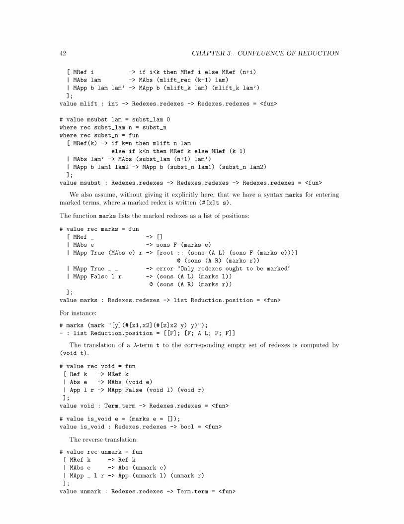
42 CHAPTER 3. CONFLUENCE OF REDUCTION
[ MRef i -> if i<k then MRef i else MRef (n+i)
| MAbs lam -> MAbs (mlift_rec (k+1) lam)
| MApp b lam lam’ -> MApp b (mlift_k lam) (mlift_k lam’)
];
value mlift : int -> Redexes.redexes -> Redexes.redexes = <fun>
# value msubst lam = subst_lam 0
where rec subst_lam n = subst_n
where rec subst_n = fun
[ MRef(k) -> if k=n then mlift n lam
else if k<n then MRef k else MRef (k-1)
| MAbs lam’ -> MAbs (subst_lam (n+1) lam’)
| MApp b lam1 lam2 -> MApp b (subst_n lam1) (subst_n lam2)
];
value msubst : Redexes.redexes -> Redexes.redexes -> Redexes.redexes = <fun>
We also assume, without giving it explicitly here, that we have a syntax marks for enteringmarked terms, where a marked redex is written (#[x]t s).
The function marks lists the marked redexes as a list of positions:
# value rec marks = fun
[ MRef _ -> []
| MAbs e -> sons F (marks e)
| MApp True (MAbs e) r -> [root :: (sons (A L) (sons F (marks e)))]
@ (sons (A R) (marks r))
| MApp True _ _ -> error "Only redexes ought to be marked"
| MApp False l r -> (sons (A L) (marks l))
@ (sons (A R) (marks r))
];
value marks : Redexes.redexes -> list Reduction.position = <fun>
For instance:
# marks (mark "[y](#[x1,x2](#[z]x2 y) y)");
- : list Reduction.position = [[F]; [F; A L; F; F]]
The translation of a λ-term t to the corresponding empty set of redexes is computed by(void t).
# value rec void = fun
[ Ref k -> MRef k
| Abs e -> MAbs (void e)
| App l r -> MApp False (void l) (void r)
];
value void : Term.term -> Redexes.redexes = <fun>
# value is_void e = (marks e = []);
value is_void : Redexes.redexes -> bool = <fun>
The reverse translation:
# value rec unmark = fun
[ MRef k -> Ref k
| MAbs e -> Abs (unmark e)
| MApp _ l r -> App (unmark l) (unmark r)
];
value unmark : Redexes.redexes -> Term.term = <fun>
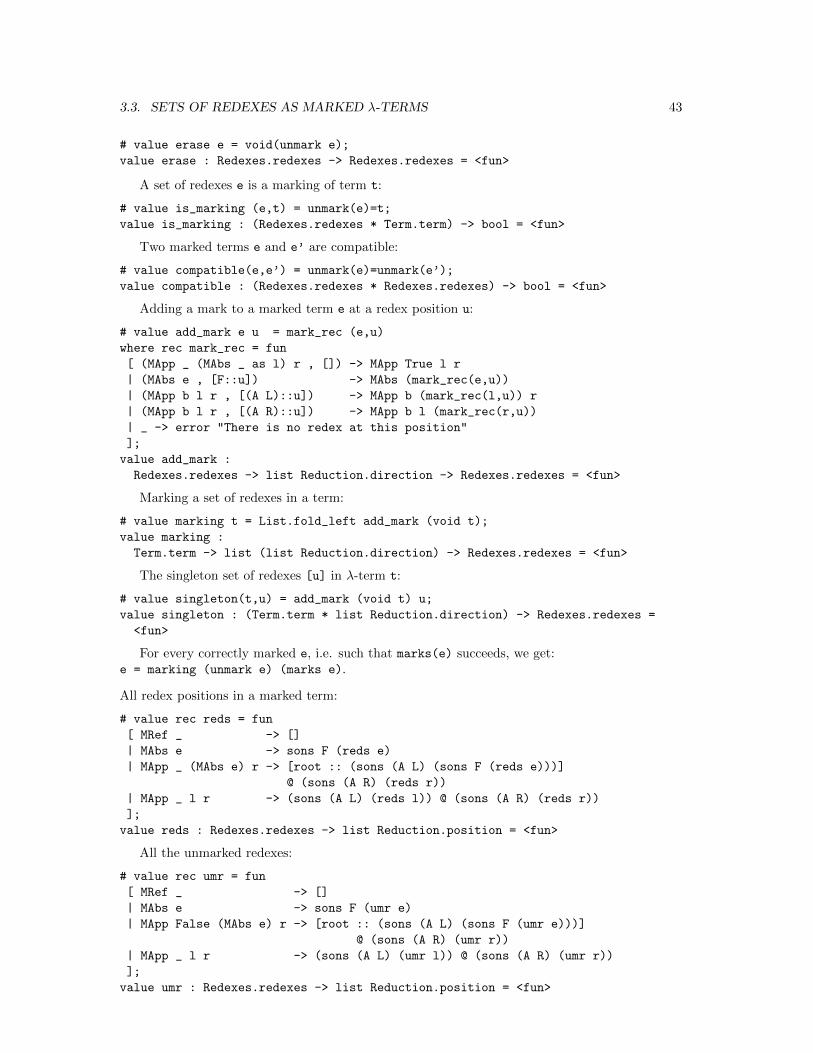
3.3. SETS OF REDEXES AS MARKED λ-TERMS 43
# value erase e = void(unmark e);
value erase : Redexes.redexes -> Redexes.redexes = <fun>
A set of redexes e is a marking of term t:
# value is_marking (e,t) = unmark(e)=t;
value is_marking : (Redexes.redexes * Term.term) -> bool = <fun>
Two marked terms e and e’ are compatible:
# value compatible(e,e’) = unmark(e)=unmark(e’);
value compatible : (Redexes.redexes * Redexes.redexes) -> bool = <fun>
Adding a mark to a marked term e at a redex position u:
# value add_mark e u = mark_rec (e,u)
where rec mark_rec = fun
[ (MApp _ (MAbs _ as l) r , []) -> MApp True l r
| (MAbs e , [F::u]) -> MAbs (mark_rec(e,u))
| (MApp b l r , [(A L)::u]) -> MApp b (mark_rec(l,u)) r
| (MApp b l r , [(A R)::u]) -> MApp b l (mark_rec(r,u))
| _ -> error "There is no redex at this position"
];
value add_mark :
Redexes.redexes -> list Reduction.direction -> Redexes.redexes = <fun>
Marking a set of redexes in a term:
# value marking t = List.fold_left add_mark (void t);
value marking :
Term.term -> list (list Reduction.direction) -> Redexes.redexes = <fun>
The singleton set of redexes [u] in λ-term t:
# value singleton(t,u) = add_mark (void t) u;
value singleton : (Term.term * list Reduction.direction) -> Redexes.redexes =
<fun>
For every correctly marked e, i.e. such that marks(e) succeeds, we get:e = marking (unmark e) (marks e).
All redex positions in a marked term:
# value rec reds = fun
[ MRef _ -> []
| MAbs e -> sons F (reds e)
| MApp _ (MAbs e) r -> [root :: (sons (A L) (sons F (reds e)))]
@ (sons (A R) (reds r))
| MApp _ l r -> (sons (A L) (reds l)) @ (sons (A R) (reds r))
];
value reds : Redexes.redexes -> list Reduction.position = <fun>
All the unmarked redexes:
# value rec umr = fun
[ MRef _ -> []
| MAbs e -> sons F (umr e)
| MApp False (MAbs e) r -> [root :: (sons (A L) (sons F (umr e)))]
@ (sons (A R) (umr r))
| MApp _ l r -> (sons (A L) (umr l)) @ (sons (A R) (umr r))
];
value umr : Redexes.redexes -> list Reduction.position = <fun>
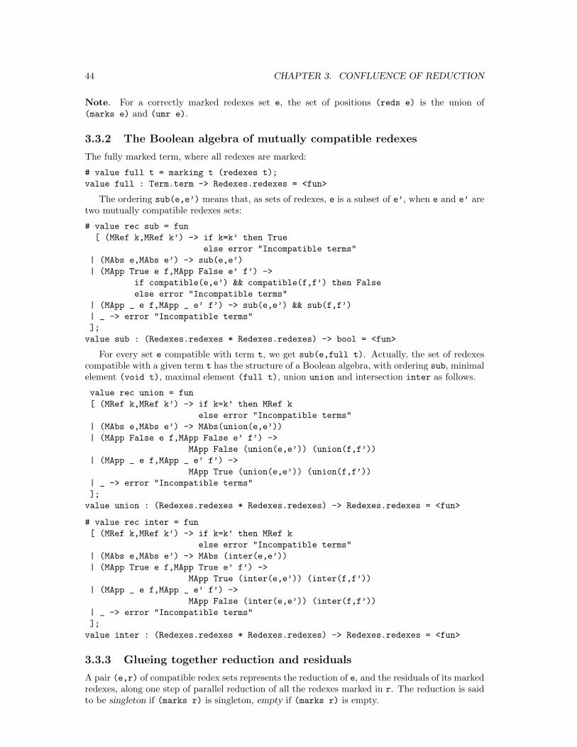
44 CHAPTER 3. CONFLUENCE OF REDUCTION
Note. For a correctly marked redexes set e, the set of positions (reds e) is the union of(marks e) and (umr e).
3.3.2 The Boolean algebra of mutually compatible redexes
The fully marked term, where all redexes are marked:
# value full t = marking t (redexes t);
value full : Term.term -> Redexes.redexes = <fun>
The ordering sub(e,e’) means that, as sets of redexes, e is a subset of e’, when e and e’ aretwo mutually compatible redexes sets:
# value rec sub = fun
[ (MRef k,MRef k’) -> if k=k’ then True
else error "Incompatible terms"
| (MAbs e,MAbs e’) -> sub(e,e’)
| (MApp True e f,MApp False e’ f’) ->
if compatible(e,e’) && compatible(f,f’) then False
else error "Incompatible terms"
| (MApp _ e f,MApp _ e’ f’) -> sub(e,e’) && sub(f,f’)
| _ -> error "Incompatible terms"
];
value sub : (Redexes.redexes * Redexes.redexes) -> bool = <fun>
For every set e compatible with term t, we get sub(e,full t). Actually, the set of redexescompatible with a given term t has the structure of a Boolean algebra, with ordering sub, minimalelement (void t), maximal element (full t), union union and intersection inter as follows.
value rec union = fun
[ (MRef k,MRef k’) -> if k=k’ then MRef k
else error "Incompatible terms"
| (MAbs e,MAbs e’) -> MAbs(union(e,e’))
| (MApp False e f,MApp False e’ f’) ->
MApp False (union(e,e’)) (union(f,f’))
| (MApp _ e f,MApp _ e’ f’) ->
MApp True (union(e,e’)) (union(f,f’))
| _ -> error "Incompatible terms"
];
value union : (Redexes.redexes * Redexes.redexes) -> Redexes.redexes = <fun>
# value rec inter = fun
[ (MRef k,MRef k’) -> if k=k’ then MRef k
else error "Incompatible terms"
| (MAbs e,MAbs e’) -> MAbs (inter(e,e’))
| (MApp True e f,MApp True e’ f’) ->
MApp True (inter(e,e’)) (inter(f,f’))
| (MApp _ e f,MApp _ e’ f’) ->
MApp False (inter(e,e’)) (inter(f,f’))
| _ -> error "Incompatible terms"
];
value inter : (Redexes.redexes * Redexes.redexes) -> Redexes.redexes = <fun>
3.3.3 Glueing together reduction and residuals
A pair (e,r) of compatible redex sets represents the reduction of e, and the residuals of its markedredexes, along one step of parallel reduction of all the redexes marked in r. The reduction is saidto be singleton if (marks r) is singleton, empty if (marks r) is empty.
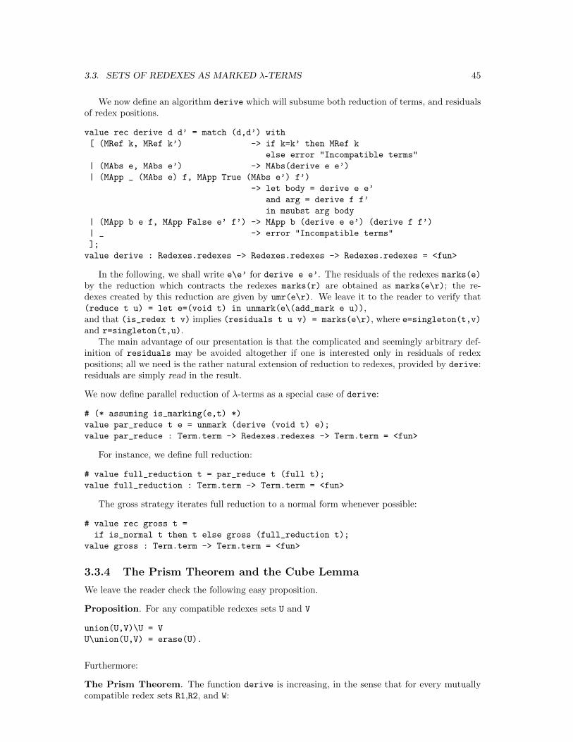
3.3. SETS OF REDEXES AS MARKED λ-TERMS 45
We now define an algorithm derive which will subsume both reduction of terms, and residualsof redex positions.
value rec derive d d’ = match (d,d’) with
[ (MRef k, MRef k’) -> if k=k’ then MRef k
else error "Incompatible terms"
| (MAbs e, MAbs e’) -> MAbs(derive e e’)
| (MApp _ (MAbs e) f, MApp True (MAbs e’) f’)
-> let body = derive e e’
and arg = derive f f’
in msubst arg body
| (MApp b e f, MApp False e’ f’) -> MApp b (derive e e’) (derive f f’)
| _ -> error "Incompatible terms"
];
value derive : Redexes.redexes -> Redexes.redexes -> Redexes.redexes = <fun>
In the following, we shall write e\e’ for derive e e’. The residuals of the redexes marks(e)by the reduction which contracts the redexes marks(r) are obtained as marks(e\r); the re-dexes created by this reduction are given by umr(e\r). We leave it to the reader to verify that(reduce t u) = let e=(void t) in unmark(e\(add_mark e u)),and that (is_redex t v) implies (residuals t u v) = marks(e\r), where e=singleton(t,v)and r=singleton(t,u).
The main advantage of our presentation is that the complicated and seemingly arbitrary def-inition of residuals may be avoided altogether if one is interested only in residuals of redexpositions; all we need is the rather natural extension of reduction to redexes, provided by derive:residuals are simply read in the result.
We now define parallel reduction of λ-terms as a special case of derive:
# (* assuming is_marking(e,t) *)
value par_reduce t e = unmark (derive (void t) e);
value par_reduce : Term.term -> Redexes.redexes -> Term.term = <fun>
For instance, we define full reduction:
# value full_reduction t = par_reduce t (full t);
value full_reduction : Term.term -> Term.term = <fun>
The gross strategy iterates full reduction to a normal form whenever possible:
# value rec gross t =
if is_normal t then t else gross (full_reduction t);
value gross : Term.term -> Term.term = <fun>
3.3.4 The Prism Theorem and the Cube Lemma
We leave the reader check the following easy proposition.
Proposition. For any compatible redexes sets U and V
union(U,V)\U = V
U\union(U,V) = erase(U).
Furthermore:
The Prism Theorem. The function derive is increasing, in the sense that for every mutuallycompatible redex sets R1,R2, and W:
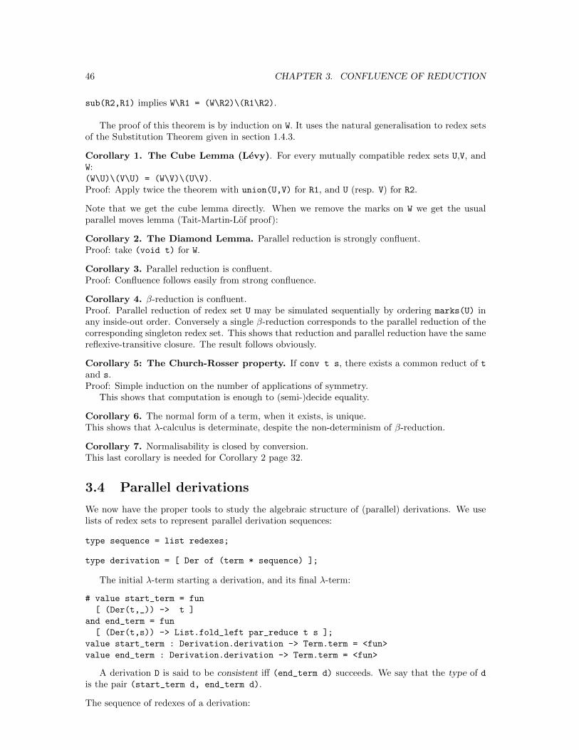
46 CHAPTER 3. CONFLUENCE OF REDUCTION
sub(R2,R1) implies W\R1 = (W\R2)\(R1\R2).
The proof of this theorem is by induction on W. It uses the natural generalisation to redex setsof the Substitution Theorem given in section 1.4.3.
Corollary 1. The Cube Lemma (Levy). For every mutually compatible redex sets U,V, andW:(W\U)\(V\U) = (W\V)\(U\V).Proof: Apply twice the theorem with union(U,V) for R1, and U (resp. V) for R2.
Note that we get the cube lemma directly. When we remove the marks on W we get the usualparallel moves lemma (Tait-Martin-Lof proof):
Corollary 2. The Diamond Lemma. Parallel reduction is strongly confluent.Proof: take (void t) for W.
Corollary 3. Parallel reduction is confluent.Proof: Confluence follows easily from strong confluence.
Corollary 4. β-reduction is confluent.Proof. Parallel reduction of redex set U may be simulated sequentially by ordering marks(U) inany inside-out order. Conversely a single β-reduction corresponds to the parallel reduction of thecorresponding singleton redex set. This shows that reduction and parallel reduction have the samereflexive-transitive closure. The result follows obviously.
Corollary 5: The Church-Rosser property. If conv t s, there exists a common reduct of tand s.Proof: Simple induction on the number of applications of symmetry.
This shows that computation is enough to (semi-)decide equality.
Corollary 6. The normal form of a term, when it exists, is unique.This shows that λ-calculus is determinate, despite the non-determinism of β-reduction.
Corollary 7. Normalisability is closed by conversion.This last corollary is needed for Corollary 2 page 32.
3.4 Parallel derivations
We now have the proper tools to study the algebraic structure of (parallel) derivations. We uselists of redex sets to represent parallel derivation sequences:
type sequence = list redexes;
type derivation = [ Der of (term * sequence) ];
The initial λ-term starting a derivation, and its final λ-term:
# value start_term = fun
[ (Der(t,_)) -> t ]
and end_term = fun
[ (Der(t,s)) -> List.fold_left par_reduce t s ];
value start_term : Derivation.derivation -> Term.term = <fun>
value end_term : Derivation.derivation -> Term.term = <fun>
A derivation D is said to be consistent iff (end_term d) succeeds. We say that the type of dis the pair (start_term d, end_term d).
The sequence of redexes of a derivation:
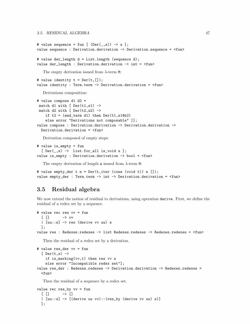
3.5. RESIDUAL ALGEBRA 47
# value sequence = fun [ (Der(_,s)) -> s ];
value sequence : Derivation.derivation -> Derivation.sequence = <fun>
# value der_length d = List.length (sequence d);
value der_length : Derivation.derivation -> int = <fun>
The empty derivation issued from λ-term M:
# value identity t = Der(t,[]);
value identity : Term.term -> Derivation.derivation = <fun>
Derivations composition:
# value compose d1 d2 =
match d1 with [ Der(t1,s1) ->
match d2 with [ Der(t2,s2) ->
if t2 = (end_term d1) then Der(t1,s1@s2)
else error "Derivations not composable" ]];
value compose : Derivation.derivation -> Derivation.derivation ->
Derivation.derivation = <fun>
Derivation composed of empty steps:
# value is_empty = fun
[ Der(_,s) -> List.for_all is_void s ];
value is_empty : Derivation.derivation -> bool = <fun>
The empty derivation of length n issued from λ-term M:
# value empty_der t n = Der(t,iter (cons (void t)) n []);
value empty_der : Term.term -> int -> Derivation.derivation = <fun>
3.5 Residual algebra
We now extend the notion of residual to derivations, using operation derive. First, we define theresidual of a redex set by a sequence.
# value rec res vv = fun
[ [] -> vv
| [uu::s] -> res (derive vv uu) s
];
value res : Redexes.redexes -> list Redexes.redexes -> Redexes.redexes = <fun>
Then the residual of a redex set by a derivation.
# value res_der vv = fun
[ Der(t,s) ->
if is_marking(vv,t) then res vv s
else error "Incompatible redex set"];
value res_der : Redexes.redexes -> Derivation.derivation -> Redexes.redexes =
<fun>
Then the residual of a sequence by a redex set.
value rec res_by vv = fun
[ [] -> []
| [uu::s] -> [(derive uu vv)::(res_by (derive vv uu) s)]
];
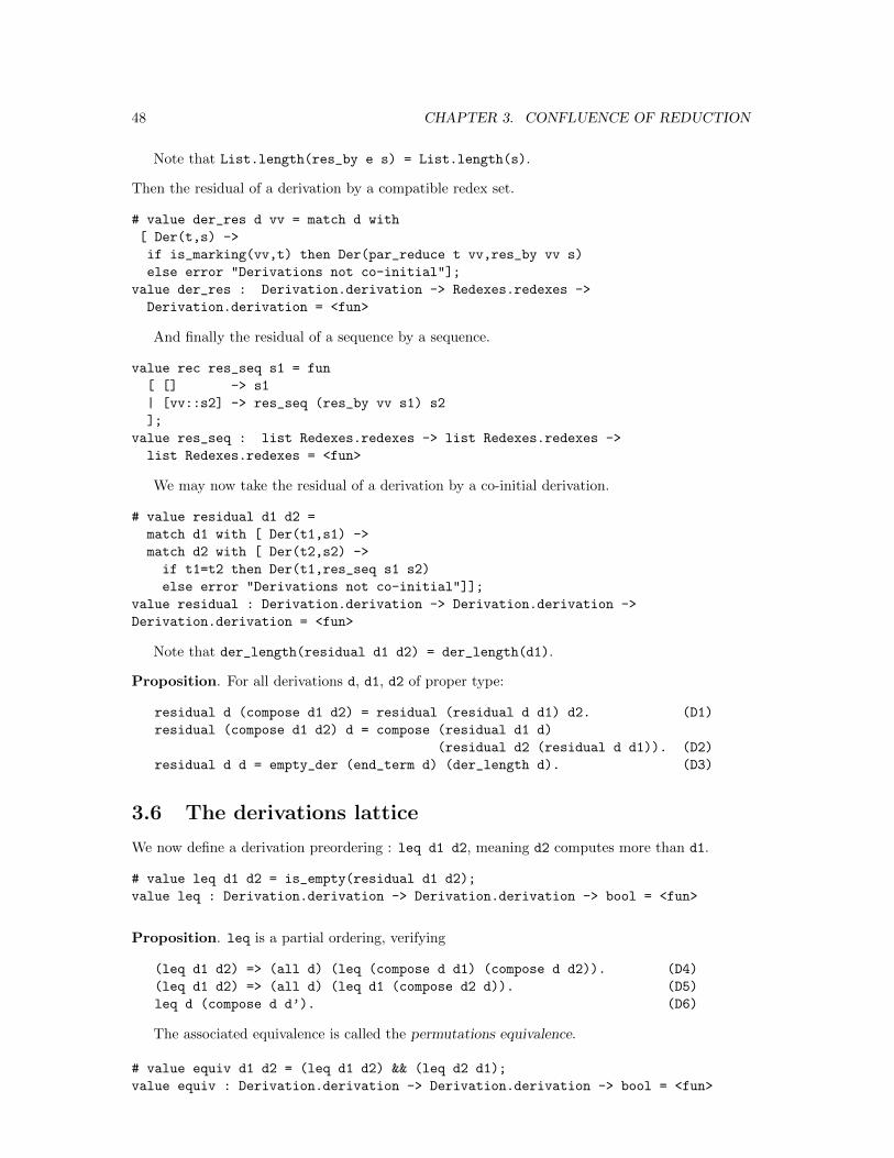
48 CHAPTER 3. CONFLUENCE OF REDUCTION
Note that List.length(res_by e s) = List.length(s).
Then the residual of a derivation by a compatible redex set.
# value der_res d vv = match d with
[ Der(t,s) ->
if is_marking(vv,t) then Der(par_reduce t vv,res_by vv s)
else error "Derivations not co-initial"];
value der_res : Derivation.derivation -> Redexes.redexes ->
Derivation.derivation = <fun>
And finally the residual of a sequence by a sequence.
value rec res_seq s1 = fun
[ [] -> s1
| [vv::s2] -> res_seq (res_by vv s1) s2
];
value res_seq : list Redexes.redexes -> list Redexes.redexes ->
list Redexes.redexes = <fun>
We may now take the residual of a derivation by a co-initial derivation.
# value residual d1 d2 =
match d1 with [ Der(t1,s1) ->
match d2 with [ Der(t2,s2) ->
if t1=t2 then Der(t1,res_seq s1 s2)
else error "Derivations not co-initial"]];
value residual : Derivation.derivation -> Derivation.derivation ->
Derivation.derivation = <fun>
Note that der_length(residual d1 d2) = der_length(d1).
Proposition. For all derivations d, d1, d2 of proper type:
residual d (compose d1 d2) = residual (residual d d1) d2. (D1)
residual (compose d1 d2) d = compose (residual d1 d)
(residual d2 (residual d d1)). (D2)
residual d d = empty_der (end_term d) (der_length d). (D3)
3.6 The derivations lattice
We now define a derivation preordering : leq d1 d2, meaning d2 computes more than d1.
# value leq d1 d2 = is_empty(residual d1 d2);
value leq : Derivation.derivation -> Derivation.derivation -> bool = <fun>
Proposition. leq is a partial ordering, verifying
(leq d1 d2) => (all d) (leq (compose d d1) (compose d d2)). (D4)
(leq d1 d2) => (all d) (leq d1 (compose d2 d)). (D5)
leq d (compose d d’). (D6)
The associated equivalence is called the permutations equivalence.
# value equiv d1 d2 = (leq d1 d2) && (leq d2 d1);
value equiv : Derivation.derivation -> Derivation.derivation -> bool = <fun>
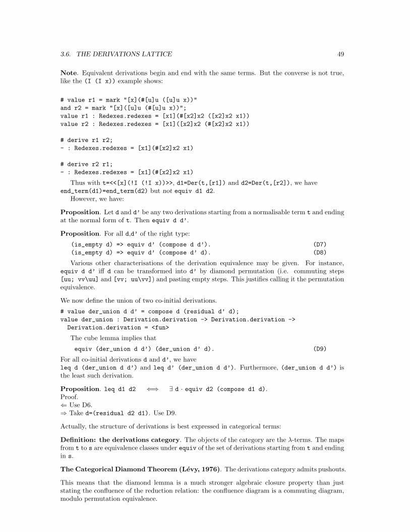
3.6. THE DERIVATIONS LATTICE 49
Note. Equivalent derivations begin and end with the same terms. But the converse is not true,like the (I (I x)) example shows:
# value r1 = mark "[x](#[u]u ([u]u x))"
and r2 = mark "[x]([u]u (#[u]u x))";
value r1 : Redexes.redexes = [x1](#[x2]x2 ([x2]x2 x1))
value r2 : Redexes.redexes = [x1]([x2]x2 (#[x2]x2 x1))
# derive r1 r2;
- : Redexes.redexes = [x1](#[x2]x2 x1)
# derive r2 r1;
- : Redexes.redexes = [x1](#[x2]x2 x1)
Thus with t=<<[x](!I (!I x))>>, d1=Der(t,[r1]) and d2=Der(t,[r2]), we haveend_term(d1)=end_term(d2) but not equiv d1 d2.
However, we have:
Proposition. Let d and d’ be any two derivations starting from a normalisable term t and endingat the normal form of t. Then equiv d d’.
Proposition. For all d,d’ of the right type:
(is_empty d) => equiv d’ (compose d d’). (D7)
(is_empty d) => equiv d’ (compose d’ d). (D8)
Various other characterisations of the derivation equivalence may be given. For instance,equiv d d’ iff d can be transformed into d’ by diamond permutation (i.e. commuting steps[uu; vv\uu] and [vv; uu\vv]) and pasting empty steps. This justifies calling it the permutationequivalence.
We now define the union of two co-initial derivations.
# value der_union d d’ = compose d (residual d’ d);
value der_union : Derivation.derivation -> Derivation.derivation ->
Derivation.derivation = <fun>
The cube lemma implies that
equiv (der_union d d’) (der_union d’ d). (D9)
For all co-initial derivations d and d’, we haveleq d (der_union d d’) and leq d’ (der_union d d’). Furthermore, (der_union d d’) isthe least such derivation.
Proposition. leq d1 d2 ⇐⇒ ∃ d · equiv d2 (compose d1 d).Proof.⇐ Use D6.⇒ Take d=(residual d2 d1). Use D9.
Actually, the structure of derivations is best expressed in categorical terms:
Definition: the derivations category. The objects of the category are the λ-terms. The mapsfrom t to s are equivalence classes under equiv of the set of derivations starting from t and endingin s.
The Categorical Diamond Theorem (Levy, 1976). The derivations category admits pushouts.
This means that the diamond lemma is a much stronger algebraic closure property than juststating the confluence of the reduction relation: the confluence diagram is a commuting diagram,modulo permutation equivalence.
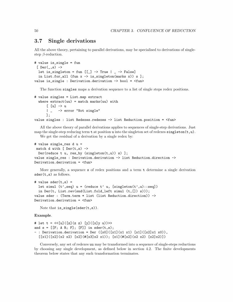
50 CHAPTER 3. CONFLUENCE OF REDUCTION
3.7 Single derivations
All the above theory, pertaining to parallel derivations, may be specialised to derivations of single-step β-reduction.
# value is_single = fun
[ Der(_,s) ->
let is_singleton = fun [[_] -> True | _ -> False]
in List.for_all (fun x -> is_singleton(marks x)) s ];
value is_single : Derivation.derivation -> bool = <fun>
The function singles maps a derivation sequence to a list of single steps redex positions.
# value singles = List.map extract
where extract(uu) = match marks(uu) with
[ [u] -> u
| _ -> error "Not single"
];
value singles : list Redexes.redexes -> list Reduction.position = <fun>
All the above theory of parallel derivations applies to sequences of single-step derivations. Justmap the single-step reducing term t at position u into the singleton set of redexes singleton(t,u).
We get the residual of a derivation by a single redex by:
# value single_res d u =
match d with [ Der(t,s) ->
Der(reduce t u, res_by (singleton(t,u)) s) ];
value single_res : Derivation.derivation -> list Reduction.direction ->
Derivation.derivation = <fun>
More generally, a sequence s of redex positions and a term t determine a single derivationsder(t,s) as follows.
# value sder(t,s) =
let simul (t’,seq) u = (reduce t’ u, [singleton(t’,u)::seq])
in Der(t, List.rev(snd(List.fold_left simul (t,[]) s)));
value sder : (Term.term * list (list Reduction.direction)) ->
Derivation.derivation = <fun>
Note that is_single(sder(t,s)).
Example.
# let t = <<[u]([z](z z) [y]([x]y u))>>
and s = [[F; A R; F]; [F]] in sder(t,s);
- : Derivation.derivation = Der ([x0]([x1](x1 x1) [x1]([x2]x1 x0)),
[[x1]([x2](x2 x2) [x2](#[x3]x2 x1)); [x1](#[x2](x2 x2) [x2]x2)])
Conversely, any set of redexes uu may be transformed into a sequence of single-steps reductionsby choosing any single development, as defined below in section 4.2. The finite developmentstheorem below states that any such transformation terminates.
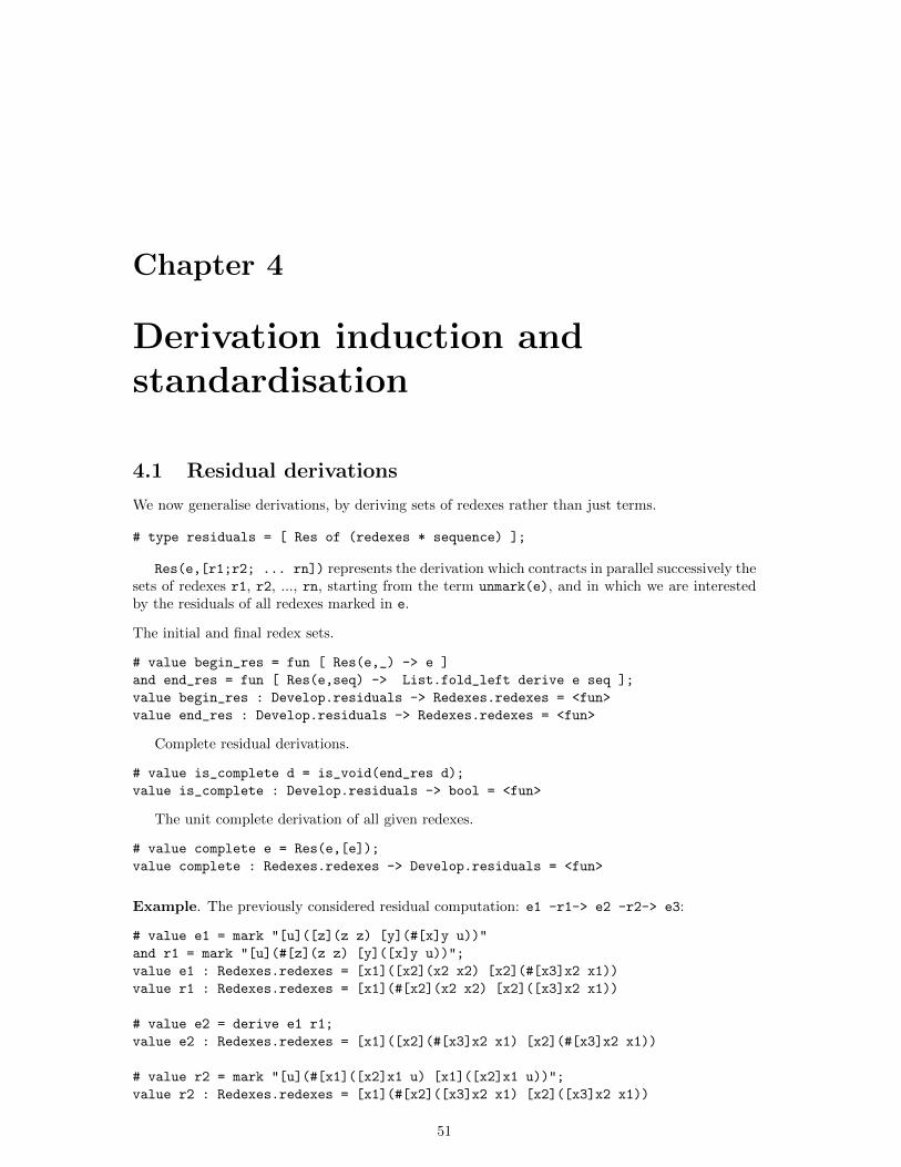
Chapter 4
Derivation induction andstandardisation
4.1 Residual derivations
We now generalise derivations, by deriving sets of redexes rather than just terms.
# type residuals = [ Res of (redexes * sequence) ];
Res(e,[r1;r2; ... rn]) represents the derivation which contracts in parallel successively thesets of redexes r1, r2, ..., rn, starting from the term unmark(e), and in which we are interestedby the residuals of all redexes marked in e.
The initial and final redex sets.
# value begin_res = fun [ Res(e,_) -> e ]
and end_res = fun [ Res(e,seq) -> List.fold_left derive e seq ];
value begin_res : Develop.residuals -> Redexes.redexes = <fun>
value end_res : Develop.residuals -> Redexes.redexes = <fun>
Complete residual derivations.
# value is_complete d = is_void(end_res d);
value is_complete : Develop.residuals -> bool = <fun>
The unit complete derivation of all given redexes.
# value complete e = Res(e,[e]);
value complete : Redexes.redexes -> Develop.residuals = <fun>
Example. The previously considered residual computation: e1 -r1-> e2 -r2-> e3:
# value e1 = mark "[u]([z](z z) [y](#[x]y u))"
and r1 = mark "[u](#[z](z z) [y]([x]y u))";
value e1 : Redexes.redexes = [x1]([x2](x2 x2) [x2](#[x3]x2 x1))
value r1 : Redexes.redexes = [x1](#[x2](x2 x2) [x2]([x3]x2 x1))
# value e2 = derive e1 r1;
value e2 : Redexes.redexes = [x1]([x2](#[x3]x2 x1) [x2](#[x3]x2 x1))
# value r2 = mark "[u](#[x1]([x2]x1 u) [x1]([x2]x1 u))";
value r2 : Redexes.redexes = [x1](#[x2]([x3]x2 x1) [x2]([x3]x2 x1))
51
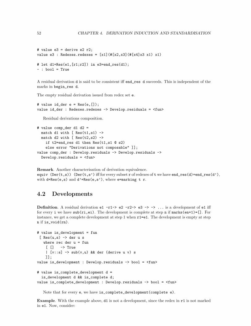
52 CHAPTER 4. DERIVATION INDUCTION AND STANDARDISATION
# value e3 = derive e2 r2;
value e3 : Redexes.redexes = [x1](#[x2,x3](#[x4]x3 x1) x1)
# let d1=Res(e1,[r1;r2]) in e3=end_res(d1);
- : bool = True
A residual derivation d is said to be consistent iff end_res d succeeds. This is independent of themarks in begin_res d.
The empty residual derivation issued from redex set e.
# value id_der e = Res(e,[]);
value id_der : Redexes.redexes -> Develop.residuals = <fun>
Residual derivations composition.
# value comp_der d1 d2 =
match d1 with [ Res(t1,s1) ->
match d2 with [ Res(t2,s2) ->
if t2=end_res d1 then Res(t1,s1 @ s2)
else error "Derivations not composable" ]];
value comp_der : Develop.residuals -> Develop.residuals ->
Develop.residuals = <fun>
Remark. Another characterisation of derivation equivalence.equiv (Der(t,s)) (Der(t,s’) iff for every subset r of redexes of t we have end_res(d)=end_res(d’),with d=Res(e,s) and d’=Res(e,s’), where e=marking t r.
4.2 Developments
Definition. A residual derivation e1 -r1-> e2 -r2-> e3 -> -> ... is a development of e1 ifffor every i we have sub(ri,ei). The development is complete at step n if marks(en+1)=[]. Forinstance, we get a complete development at step 1 when r1=e1. The development is empty at stepn if is_void(rn).
# value is_development = fun
[ Res(u,s) -> der u s
where rec der u = fun
[ [] -> True
| [v::s] -> sub(v,u) && der (derive u v) s
]];
value is_development : Develop.residuals -> bool = <fun>
# value is_complete_development d =
is_development d && is_complete d;
value is_complete_development : Develop.residuals -> bool = <fun>
Note that for every e, we have is_complete_development(complete e).
Example. With the example above, d1 is not a development, since the redex in r1 is not markedin e1. Now, consider:
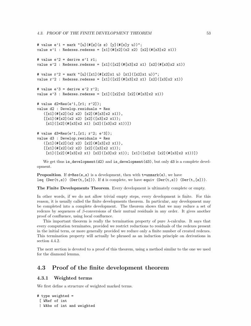
4.3. PROOF OF THE FINITE DEVELOPMENT THEOREM 53
# value e’1 = mark "[u](#[z](z z) [y](#[x]y u))";
value e’1 : Redexes.redexes = [x1](#[x2](x2 x2) [x2](#[x3]x2 x1))
# value e’2 = derive e’1 r1;
value e’2 : Redexes.redexes = [x1]([x2](#[x3]x2 x1) [x2](#[x3]x2 x1))
# value r’2 = mark "[u]([x1](#[x2]x1 u) [x1]([x2]x1 u))";
value r’2 : Redexes.redexes = [x1]([x2](#[x3]x2 x1) [x2]([x3]x2 x1))
# value e’3 = derive e’2 r’2;
value e’3 : Redexes.redexes = [x1]([x2]x2 [x2](#[x3]x2 x1))
# value d2=Res(e’1,[r1; r’2]);
value d2 : Develop.residuals = Res
([x1](#[x2](x2 x2) [x2](#[x3]x2 x1)),
[[x1](#[x2](x2 x2) [x2]([x3]x2 x1));
[x1]([x2](#[x3]x2 x1) [x2]([x3]x2 x1))])
# value d3=Res(e’1,[r1; r’2; e’3]);
value d3 : Develop.residuals = Res
([x1](#[x2](x2 x2) [x2](#[x3]x2 x1)),
[[x1](#[x2](x2 x2) [x2]([x3]x2 x1));
[x1]([x2](#[x3]x2 x1) [x2]([x3]x2 x1)); [x1]([x2]x2 [x2](#[x3]x2 x1))])
We get thus is_development(d2) and is_development(d3), but only d3 is a complete devel-opment.
Proposition. If d=Res(e,s) is a development, then with t=unmark(e), we haveleq (Der(t,s)) (Der(t,[e])). If d is complete, we have equiv (Der(t,s)) (Der(t,[e])).
The Finite Developments Theorem. Every development is ultimately complete or empty.
In other words, if we do not allow trivial empty steps, every development is finite. For thisreason, it is usually called the finite developments theorem. In particular, any development maybe completed into a complete development. The theorem shows that we may reduce a set ofredexes by sequences of β-conversions of their mutual residuals in any order. It gives anotherproof of confluence, using local confluence.
This important theorem is really the termination property of pure λ-calculus. It says thatevery computation terminates, provided we restrict reductions to residuals of the redexes presentin the initial term, or more generally provided we reduce only a finite number of created redexes.This termination property will actually be phrased as an induction principle on derivations insection 4.4.2.
The next section is devoted to a proof of this theorem, using a method similar to the one we usedfor the diamond lemma.
4.3 Proof of the finite development theorem
4.3.1 Weighted terms
We first define a structure of weighted marked terms.
# type weighted =
[ WRef of int
| WAbs of int and weighted
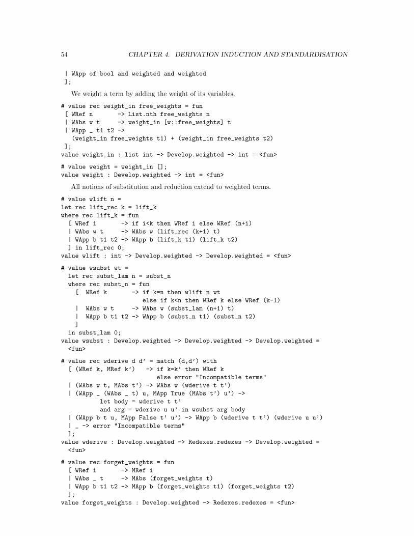
54 CHAPTER 4. DERIVATION INDUCTION AND STANDARDISATION
| WApp of bool and weighted and weighted
];
We weight a term by adding the weight of its variables.
# value rec weight_in free_weights = fun
[ WRef n -> List.nth free_weights n
| WAbs w t -> weight_in [w::free_weights] t
| WApp _ t1 t2 ->
(weight_in free_weights t1) + (weight_in free_weights t2)
];
value weight_in : list int -> Develop.weighted -> int = <fun>
# value weight = weight_in [];
value weight : Develop.weighted -> int = <fun>
All notions of substitution and reduction extend to weighted terms.
# value wlift n =
let rec lift_rec k = lift_k
where rec lift_k = fun
[ WRef i -> if i<k then WRef i else WRef (n+i)
| WAbs w t -> WAbs w (lift_rec (k+1) t)
| WApp b t1 t2 -> WApp b (lift_k t1) (lift_k t2)
] in lift_rec 0;
value wlift : int -> Develop.weighted -> Develop.weighted = <fun>
# value wsubst wt =
let rec subst_lam n = subst_n
where rec subst_n = fun
[ WRef k -> if k=n then wlift n wt
else if k<n then WRef k else WRef (k-1)
| WAbs w t -> WAbs w (subst_lam (n+1) t)
| WApp b t1 t2 -> WApp b (subst_n t1) (subst_n t2)
]
in subst_lam 0;
value wsubst : Develop.weighted -> Develop.weighted -> Develop.weighted =
<fun>
# value rec wderive d d’ = match (d,d’) with
[ (WRef k, MRef k’) -> if k=k’ then WRef k
else error "Incompatible terms"
| (WAbs w t, MAbs t’) -> WAbs w (wderive t t’)
| (WApp _ (WAbs _ t) u, MApp True (MAbs t’) u’) ->
let body = wderive t t’
and arg = wderive u u’ in wsubst arg body
| (WApp b t u, MApp False t’ u’) -> WApp b (wderive t t’) (wderive u u’)
| _ -> error "Incompatible terms"
];
value wderive : Develop.weighted -> Redexes.redexes -> Develop.weighted =
<fun>
# value rec forget_weights = fun
[ WRef i -> MRef i
| WAbs _ t -> MAbs (forget_weights t)
| WApp b t1 t2 -> MApp b (forget_weights t1) (forget_weights t2)
];
value forget_weights : Develop.weighted -> Redexes.redexes = <fun>
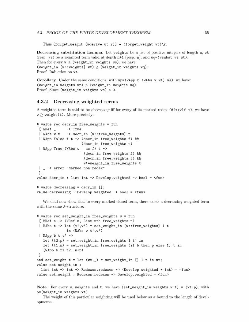
4.3. PROOF OF THE FINITE DEVELOPMENT THEOREM 55
Thus (forget_weight (wderive wt r)) = (forget_weight wt)\r.
Decreasing substitution Lemma. Let weights be a list of positive integers of length n, wt(resp. ws) be a weighted term valid at depth n+1 (resp. n), and wq=(wsubst ws wt).Then for every w ≥ (weight_in weights ws), we have:(weight_in [w::weights] wt) ≥ (weight_in weights wq).Proof: Induction on wt.
Corollary. Under the same conditions, with wp=(WApp b (WAbs w wt) ws), we have:(weight_in weights wp) > (weight_in weights wq).Proof. Since (weight_in weights ws) > 0.
4.3.2 Decreasing weighted terms
A weighted term is said to be decreasing iff for every of its marked redex (#[x:w]f t), we havew ≥ weight(t). More precisely:
# value rec decr_in free_weights = fun
[ WRef _ -> True
| WAbs w t -> decr_in [w::free_weights] t
| WApp False f t -> (decr_in free_weights f) &&
(decr_in free_weights t)
| WApp True (WAbs w _ as f) t ->
(decr_in free_weights f) &&
(decr_in free_weights t) &&
w>=weight_in free_weights t
| _ -> error "Marked non-redex"
];
value decr_in : list int -> Develop.weighted -> bool = <fun>
# value decreasing = decr_in [];
value decreasing : Develop.weighted -> bool = <fun>
We shall now show that to every marked closed term, there exists a decreasing weighted termwith the same λ-structure.
# value rec set_weight_in free_weights w = fun
[ MRef n -> (WRef n, List.nth free_weights n)
| MAbs t -> let (t’,w’) = set_weight_in [w::free_weights] 1 t
in (WAbs w t’,w’)
| MApp b t t’ ->
let (t2,p) = set_weight_in free_weights 1 t’ in
let (t1,n) = set_weight_in free_weights (if b then p else 1) t in
(WApp b t1 t2, n+p)
]
and set_weight t = let (wt,_) = set_weight_in [] 1 t in wt;
value set_weight_in :
list int -> int -> Redexes.redexes -> (Develop.weighted * int) = <fun>
value set_weight : Redexes.redexes -> Develop.weighted = <fun>
Note. For every w, weights and t, we have (set_weight_in weights w t) = (wt,p), withp=(weight_in weights wt).
The weight of this particular weighting will be used below as a bound to the length of devel-opments.
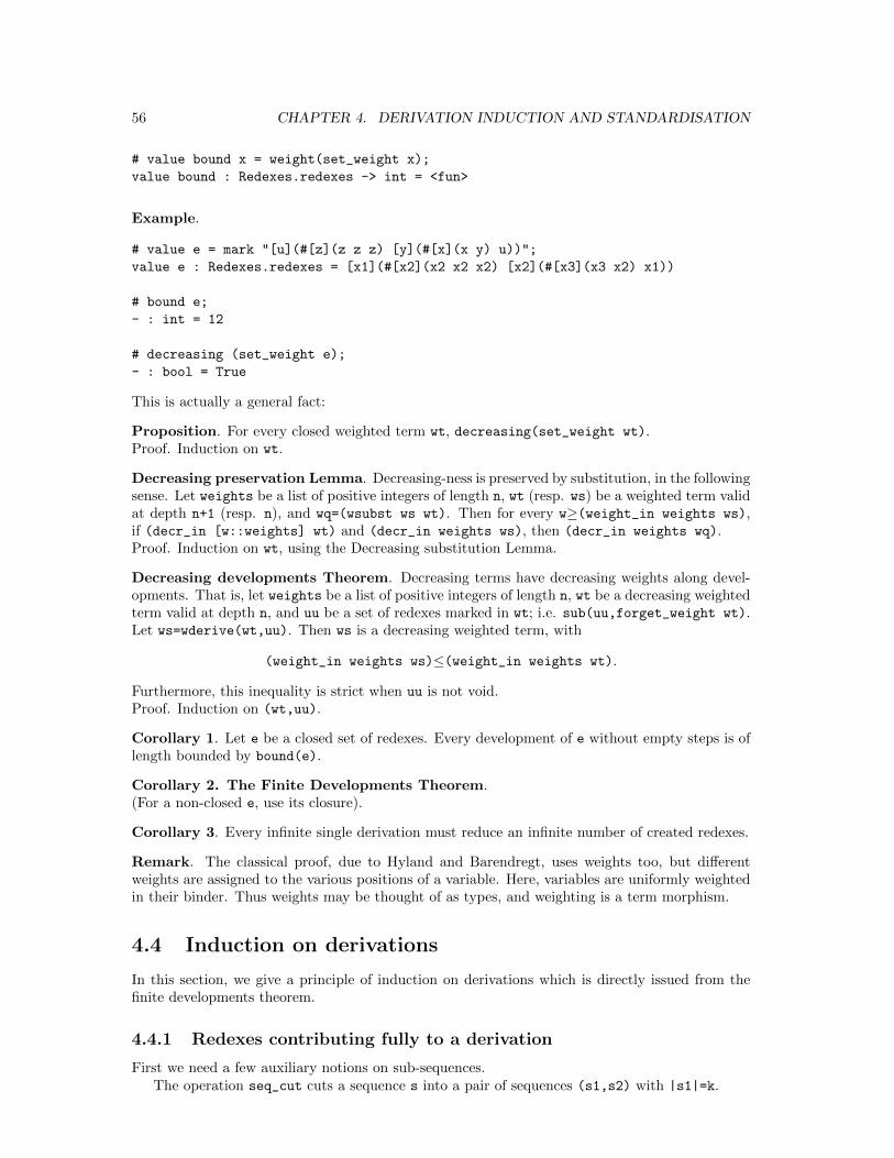
56 CHAPTER 4. DERIVATION INDUCTION AND STANDARDISATION
# value bound x = weight(set_weight x);
value bound : Redexes.redexes -> int = <fun>
Example.
# value e = mark "[u](#[z](z z z) [y](#[x](x y) u))";
value e : Redexes.redexes = [x1](#[x2](x2 x2 x2) [x2](#[x3](x3 x2) x1))
# bound e;
- : int = 12
# decreasing (set_weight e);
- : bool = True
This is actually a general fact:
Proposition. For every closed weighted term wt, decreasing(set_weight wt).Proof. Induction on wt.
Decreasing preservation Lemma. Decreasing-ness is preserved by substitution, in the followingsense. Let weights be a list of positive integers of length n, wt (resp. ws) be a weighted term validat depth n+1 (resp. n), and wq=(wsubst ws wt). Then for every w≥(weight_in weights ws),if (decr_in [w::weights] wt) and (decr_in weights ws), then (decr_in weights wq).Proof. Induction on wt, using the Decreasing substitution Lemma.
Decreasing developments Theorem. Decreasing terms have decreasing weights along devel-opments. That is, let weights be a list of positive integers of length n, wt be a decreasing weightedterm valid at depth n, and uu be a set of redexes marked in wt; i.e. sub(uu,forget_weight wt).Let ws=wderive(wt,uu). Then ws is a decreasing weighted term, with
(weight_in weights ws)≤(weight_in weights wt).
Furthermore, this inequality is strict when uu is not void.Proof. Induction on (wt,uu).
Corollary 1. Let e be a closed set of redexes. Every development of e without empty steps is oflength bounded by bound(e).
Corollary 2. The Finite Developments Theorem.(For a non-closed e, use its closure).
Corollary 3. Every infinite single derivation must reduce an infinite number of created redexes.
Remark. The classical proof, due to Hyland and Barendregt, uses weights too, but differentweights are assigned to the various positions of a variable. Here, variables are uniformly weightedin their binder. Thus weights may be thought of as types, and weighting is a term morphism.
4.4 Induction on derivations
In this section, we give a principle of induction on derivations which is directly issued from thefinite developments theorem.
4.4.1 Redexes contributing fully to a derivation
First we need a few auxiliary notions on sub-sequences.The operation seq_cut cuts a sequence s into a pair of sequences (s1,s2) with |s1|=k.
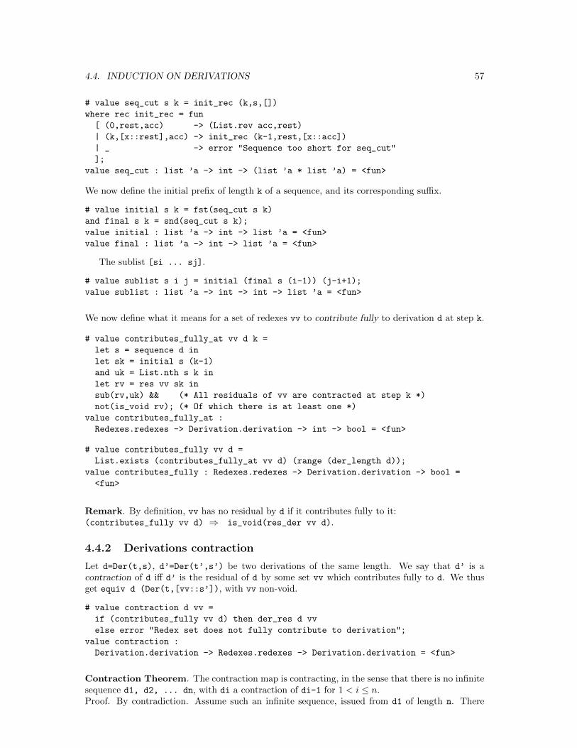
4.4. INDUCTION ON DERIVATIONS 57
# value seq_cut s k = init_rec (k,s,[])
where rec init_rec = fun
[ (0,rest,acc) -> (List.rev acc,rest)
| (k,[x::rest],acc) -> init_rec (k-1,rest,[x::acc])
| _ -> error "Sequence too short for seq_cut"
];
value seq_cut : list ’a -> int -> (list ’a * list ’a) = <fun>
We now define the initial prefix of length k of a sequence, and its corresponding suffix.
# value initial s k = fst(seq_cut s k)
and final s k = snd(seq_cut s k);
value initial : list ’a -> int -> list ’a = <fun>
value final : list ’a -> int -> list ’a = <fun>
The sublist [si ... sj].
# value sublist s i j = initial (final s (i-1)) (j-i+1);
value sublist : list ’a -> int -> int -> list ’a = <fun>
We now define what it means for a set of redexes vv to contribute fully to derivation d at step k.
# value contributes_fully_at vv d k =
let s = sequence d in
let sk = initial s (k-1)
and uk = List.nth s k in
let rv = res vv sk in
sub(rv,uk) && (* All residuals of vv are contracted at step k *)
not(is_void rv); (* Of which there is at least one *)
value contributes_fully_at :
Redexes.redexes -> Derivation.derivation -> int -> bool = <fun>
# value contributes_fully vv d =
List.exists (contributes_fully_at vv d) (range (der_length d));
value contributes_fully : Redexes.redexes -> Derivation.derivation -> bool =
<fun>
Remark. By definition, vv has no residual by d if it contributes fully to it:(contributes_fully vv d) ⇒ is_void(res_der vv d).
4.4.2 Derivations contraction
Let d=Der(t,s), d’=Der(t’,s’) be two derivations of the same length. We say that d’ is acontraction of d iff d’ is the residual of d by some set vv which contributes fully to d. We thusget equiv d (Der(t,[vv::s’]), with vv non-void.
# value contraction d vv =
if (contributes_fully vv d) then der_res d vv
else error "Redex set does not fully contribute to derivation";
value contraction :
Derivation.derivation -> Redexes.redexes -> Derivation.derivation = <fun>
Contraction Theorem. The contraction map is contracting, in the sense that there is no infinitesequence d1, d2, ... dn, with di a contraction of di-1 for 1 < i ≤ n.Proof. By contradiction. Assume such an infinite sequence, issued from d1 of length n. There
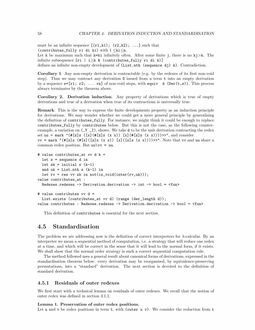
58 CHAPTER 4. DERIVATION INDUCTION AND STANDARDISATION
must be an infinite sequence [(r1,k1); (r2,k2); ...] such that(contributes_fully ri di ki) with 1 ≤ki≤n.Let k be maximum such that k=ki infinitely often. After some finite j, there is no kj>k. Theinfinite subsequence [ri | i≥k & (contributes_fully ri di k)]
defines an infinite non-empty development of (List.nth (sequence dj) k). Contradiction.
Corollary 1. Any non-empty derivation is contractable (e.g. by the redexes of its first non-voidstep). Thus we may contract any derivation D issued from a term t into an empty derivationby a sequence s=[r1; r2; ... rn] of non-void steps, with equiv d (Der(t,s)). This processalways terminates by the theorem above.
Corollary 2. Derivation induction. Any property of derivations which is true of emptyderivations and true of a derivation when true of its contractions is universally true.
Remark. This is the way to express the finite developments property as an induction principlefor derivations. We may wonder whether we could get a more general principle by generalisingthe definition of contributes_fully. For instance, we might think it could be enough to replacecontributes_fully by contributes below. But this is not the case, as the following counter-example, a variation on (_Y _I), shows. We take d to be the unit derivation contracting the redexset uu = mark "(#[z]z ([x](#[z]z (x x)) [x](#[z]z (x x))))>>", and considervv = mark "(#[z]z (#[x]([z]z (x x)) [x]([z]z (x x))))>>". Note that vv and uu share acommon redex position. But uu\vv = uu.
# value contributes_at vv d k =
let s = sequence d in
let sk = initial s (k-1)
and uk = List.nth s (k-1) in
let rv = res vv sk in not(is_void(inter(rv,uk)));
value contributes_at :
Redexes.redexes -> Derivation.derivation -> int -> bool = <fun>
# value contributes vv d =
List.exists (contributes_at vv d) (range (der_length d));
value contributes : Redexes.redexes -> Derivation.derivation -> bool = <fun>
This definition of contributes is essential for the next section.
4.5 Standardisation
The problem we are addressing now is the definition of correct interpreters for λ-calculus. By aninterpreter we mean a sequential method of computation, i.e. a strategy that will reduce one redexat a time, and which will be correct in the sense that it will lead to the normal form, if it exists.We shall show that the normal order strategy is such a correct sequential computation rule.
The method followed uses a general result about canonical forms of derivations, expressed in thestandardisation theorem below: every derivation may be reorganised, by equivalence-preservingpermutations, into a “standard” derivation. The next section is devoted to the definition ofstandard derivation.
4.5.1 Residuals of outer redexes
We first start with a technical lemma on residuals of outer redexes. We recall that the notion ofouter redex was defined in section 3.1.1.
Lemma 1. Preservation of outer redex positions.Let u and v be redex positions in term t, with (outer u v). We consider the reduction from t
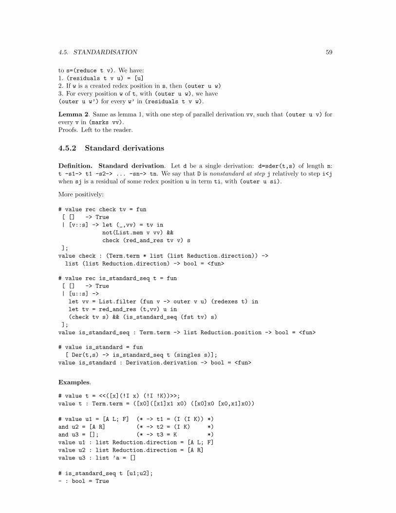
4.5. STANDARDISATION 59
to s=(reduce t v). We have:1. (residuals t v u) = [u]
2. If w is a created redex position in s, then (outer u w)
3. For every position w of t, with (outer u w), we have(outer u w’) for every w’ in (residuals t v w).
Lemma 2. Same as lemma 1, with one step of parallel derivation vv, such that (outer u v) forevery v in (marks vv).Proofs. Left to the reader.
4.5.2 Standard derivations
Definition. Standard derivation. Let d be a single derivation: d=sder(t,s) of length n:t -s1-> t1 -s2-> ... -sn-> tn. We say that D is nonstandard at step j relatively to step i<j
when sj is a residual of some redex position u in term ti, with (outer u si).
More positively:
# value rec check tv = fun
[ [] -> True
| [v::s] -> let (_,vv) = tv in
not(List.mem v vv) &&
check (red_and_res tv v) s
];
value check : (Term.term * list (list Reduction.direction)) ->
list (list Reduction.direction) -> bool = <fun>
# value rec is_standard_seq t = fun
[ [] -> True
| [u::s] ->
let vv = List.filter (fun v -> outer v u) (redexes t) in
let tv = red_and_res (t,vv) u in
(check tv s) && (is_standard_seq (fst tv) s)
];
value is_standard_seq : Term.term -> list Reduction.position -> bool = <fun>
# value is_standard = fun
[ Der(t,s) -> is_standard_seq t (singles s)];
value is_standard : Derivation.derivation -> bool = <fun>
Examples.
# value t = <<([x](!I x) (!I !K))>>;
value t : Term.term = ([x0]([x1]x1 x0) ([x0]x0 [x0,x1]x0))
# value u1 = [A L; F] (* -> t1 = (I (I K)) *)
and u2 = [A R] (* -> t2 = (I K) *)
and u3 = []; (* -> t3 = K *)
value u1 : list Reduction.direction = [A L; F]
value u2 : list Reduction.direction = [A R]
value u3 : list ’a = []
# is_standard_seq t [u1;u2];
- : bool = True
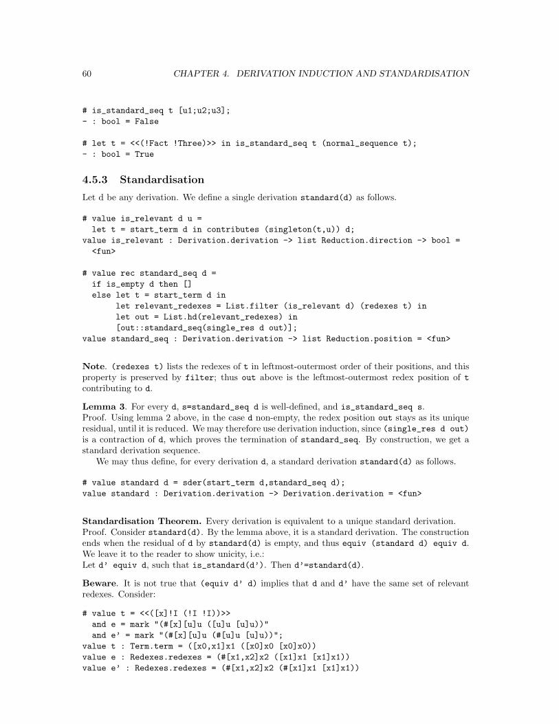
60 CHAPTER 4. DERIVATION INDUCTION AND STANDARDISATION
# is_standard_seq t [u1;u2;u3];
- : bool = False
# let t = <<(!Fact !Three)>> in is_standard_seq t (normal_sequence t);
- : bool = True
4.5.3 Standardisation
Let d be any derivation. We define a single derivation standard(d) as follows.
# value is_relevant d u =
let t = start_term d in contributes (singleton(t,u)) d;
value is_relevant : Derivation.derivation -> list Reduction.direction -> bool =
<fun>
# value rec standard_seq d =
if is_empty d then []
else let t = start_term d in
let relevant_redexes = List.filter (is_relevant d) (redexes t) in
let out = List.hd(relevant_redexes) in
[out::standard_seq(single_res d out)];
value standard_seq : Derivation.derivation -> list Reduction.position = <fun>
Note. (redexes t) lists the redexes of t in leftmost-outermost order of their positions, and thisproperty is preserved by filter; thus out above is the leftmost-outermost redex position of t
contributing to d.
Lemma 3. For every d, s=standard_seq d is well-defined, and is_standard_seq s.Proof. Using lemma 2 above, in the case d non-empty, the redex position out stays as its uniqueresidual, until it is reduced. We may therefore use derivation induction, since (single_res d out)
is a contraction of d, which proves the termination of standard_seq. By construction, we get astandard derivation sequence.
We may thus define, for every derivation d, a standard derivation standard(d) as follows.
# value standard d = sder(start_term d,standard_seq d);
value standard : Derivation.derivation -> Derivation.derivation = <fun>
Standardisation Theorem. Every derivation is equivalent to a unique standard derivation.Proof. Consider standard(d). By the lemma above, it is a standard derivation. The constructionends when the residual of d by standard(d) is empty, and thus equiv (standard d) equiv d.We leave it to the reader to show unicity, i.e.:Let d’ equiv d, such that is_standard(d’). Then d’=standard(d).
Beware. It is not true that (equiv d’ d) implies that d and d’ have the same set of relevantredexes. Consider:
# value t = <<([x]!I (!I !I))>>
and e = mark "(#[x][u]u ([u]u [u]u))"
and e’ = mark "(#[x][u]u (#[u]u [u]u))";
value t : Term.term = ([x0,x1]x1 ([x0]x0 [x0]x0))
value e : Redexes.redexes = (#[x1,x2]x2 ([x1]x1 [x1]x1))
value e’ : Redexes.redexes = (#[x1,x2]x2 (#[x1]x1 [x1]x1))
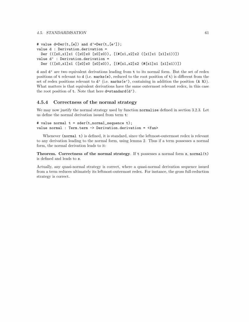
4.5. STANDARDISATION 61
# value d=Der(t,[e]) and d’=Der(t,[e’]);
value d : Derivation.derivation =
Der (([x0,x1]x1 ([x0]x0 [x0]x0)), [(#[x1,x2]x2 ([x1]x1 [x1]x1))])
value d’ : Derivation.derivation =
Der (([x0,x1]x1 ([x0]x0 [x0]x0)), [(#[x1,x2]x2 (#[x1]x1 [x1]x1))])
d and d’ are two equivalent derivations leading from t to its normal form. But the set of redexpositions of t relevant to d (i.e. marks(e), reduced to the root position of t) is different from theset of redex positions relevant to d’ (i.e. marks(e’), containing in addition the position (A R)).What matters is that equivalent derivations have the same outermost relevant redex, in this casethe root position of t. Note that here d=standard(d’).
4.5.4 Correctness of the normal strategy
We may now justify the normal strategy used by function normalise defined in section 3.2.3. Letus define the normal derivation issued from term t:
# value normal t = sder(t,normal_sequence t);
value normal : Term.term -> Derivation.derivation = <fun>
Whenever (normal t) is defined, it is standard, since the leftmost-outermost redex is relevantto any derivation leading to the normal form, using lemma 2. Thus if a term possesses a normalform, the normal derivation leads to it:
Theorem. Correctness of the normal strategy. If t possesses a normal form s, normal(t)is defined and leads to s.
Actually, any quasi-normal strategy is correct, where a quasi-normal derivation sequence issuedfrom a term reduces ultimately its leftmost-outermost redex. For instance, the gross full-reductionstrategy is correct.

62 CHAPTER 4. DERIVATION INDUCTION AND STANDARDISATION
Chapter 5
Separability
In this chapter, we shall prove a very important theorem of pure λ-calculus, the separabilitytheorem of C. Bohm. This result is the key to understanding the various semantic choices whichdistinguish possible models of λ-calculus.
Before presenting this theorem, we must develop the notions of η-conversion and Bohm trees.
5.1 Extensionality: η-conversion
The rule of η-conversion is a syntactic version of the property of extensionality. It is consistentwith the interpretation of λ-terms as denoting functions. η-conversion will be explained as thesymmetric closure of a second reduction rule, traditionally called η-reduction.
An η redex is a subterm of the form [x](M x), with x not appearing free in M. η-reductionconsists in replacing this subterm by M. In abstract form, we replace Abs(App(lift 1 M, Ref 0))
by M. The symmetric relation is called η-expansion.
# value is_eta_redex t u = match subterm(t,u) with
[ Abs (App f (Ref 0)) -> try let _ = unlift1 f in True
with [ Occurs_free -> False ]
| _ -> False
];
value is_eta_redex : Term.term -> list Reduction.direction -> bool = <fun>
# value eta_reduce t u = match subterm(t,u) with
[ Abs (App f (Ref 0)) -> try replace (unlift1 f) (t,u)
with [ Occurs_free -> error "Not an eta redex" ]
| _ -> error "Not an eta redex"
];
value eta_reduce : Term.term -> list Reduction.direction -> Term.term = <fun>
Lemma 1. η-reduction is confluent and terminating.Proof. Left to the reader.
Lemma 2. βη-reduction is confluent.Proof. See Barendregt.
# value eta_redexes t = List.filter (is_eta_redex t) (dom t);
value eta_redexes : Term.term -> list Reduction.position = <fun>
# value ered t = List.map (eta_reduce t) (eta_redexes t);
value ered : Term.term -> list Term.term = <fun>
63
64 CHAPTER 5. SEPARABILITY
η-conversion is the equivalence closure of eta reduction.
# value eta_conv = common_reduct ered;
value eta_conv : (Term.term * Term.term) -> bool = <fun>
5.2 Head normal forms and solvability
We are now convinced of the correctness of the normal interpreter. However, it is not reasonablecomputationally to iterate the search for the left-most outermost redex repeatedly from the rootof the term, since there is a sense in which outermost computations reach approximations whichare invariant by further reduction. This intuition is captured by the notion of head normal form.
5.2.1 Head normal forms
We are already familiar with the notion of head-normal form, as obtained by the result of functionhnf given in section 1.5.1 above. We recall that a head normal form is any term t of the form[x1, ..., xn](x t1 ... tp), with n,p≥ 0.Note that if red t s, then s = [x1, ..., xn](x s1 ... sp). Thus n, x, and p are invariantby β-reduction.
Remark. Every term is either a head normal form, or of the form:[x1, ..., xn](r t1 ... tp), with r a redex. In this case r is called the head redex of the term.
We now give an explicit type to head normal forms.
# type head = [ Head of (int * int * list term) ];
Remark. In Head(n,x,seq), the first integer n is the length of the abstraction prefix, whereasthe second one x is the reference index of the head variable.
Now we can reduce a λ-term to its head normal form, when it has one, by the normal reduction.Compare with algorithm hnf above.
# value head_normal = head 0 []
where rec head n args = fun
[ Ref x -> Head(n,x,args)
| Abs t -> match args with
[ [] -> head (n+1) [] t
| [a::r] -> head n r (subst a t)
]
| App f x -> head n [x::args] f
];
value head_normal : Term.term -> Bohm.head = <fun>
We say that a λ-term t is defined iff head_normal(t) terminates.
Proposition 1. If (t s) is defined, so is t. If [x]t is defined, so is t.
Proposition 2. If t is defined, the normal reduction issued from t has an initial sequence whichreduces t to s=(hnf t), and s is the first head normal form in the reduction sequence.
5.2.2 Solvability
Let us note below {t} for closure(t).
5.3. BOHM TREES 65
Definition. A λ-term t is said to be solvable iff there exist n terms c1 c2 ... cn such that({t} c1 ... cn) conv _I.
Wadsworth’s Theorem. A λ-term is defined iff it is solvable.Proof. Let t be a λ-term, which we may assume to be closed. If it is solvable, it is defined, bystandardisation and proposition 1 above. Conversely, let us assume:t red [x1, ..., xn](x t1 ... tp). Taking K_ p = [x, y1, ..., yp]x, and KpI = K_ p _I,we get: (t KpI_1 ... KpI_n) red (KpI t1 ... tp) red _I.
5.2.3 A normal interpreter
We may now organise the normal interpreter into iterating head_normal:
# type normal = [ Normal of (int * int * list normal) ];
Type normal is defined
# value rec norm t =
match head_normal t
with [ Head(n,x,args) -> Normal(n,x,List.map norm args) ];
value norm : Term.term -> Bohm.normal = <fun>
Discussion. Now norm (or equivalently nf as a function mapping λ-terms to λ-terms) looks forredexes in a top-down manner, but without exploring the initial part of the term which is formedby layers of head normal forms, and which is invariant. But these procedures will loop on termswithout normal forms. We shall now see how to compute progressively successive approximationsof a term, in a potentially infinite partial structure called the Bohm tree of the λ-term. Each nodein the tree corresponds to one layer of head normal form. Bohm trees are the natural generalisationof normal forms to infinite trees.
5.3 Bohm trees
A Bohm tree is a possibly infinite tree representing the limit of all computations issued from a giventerm. It consists of layers of approximations, each approximation corresponding to a head-normalform.
First of all we shall profit of the additional structure of head normal forms to represent variablesin a better way. Every variable is represented by a double key Index(k,i) where k addressesupwards the hnf layer where the variable is declared, while i indexes in the corresponding list ofbound variables the variable in a left to right fashion. Thus in [x1,x2,...,xn]xi(...) the headvariable is represented as Index(0,i). Note that this representation of head variables is invariantby head η-expansion.
# type var = [ Index of (int * int) ];
# type bohm = [ Hnf of (int * var * list bohm)
| Future of term
];
There are two sorts of nodes in a Bohm tree approximant: Hnf nodes, where one hnf ap-proximation has been computed, and Future nodes, containing a λ-term waiting to be examined.When this term is undefined the tree cannot be grown further in this direction. Thus Future(t)
is a sort of syntactic “bottom” meaning “not yet defined”. Any term may be transformed into aBohm tree approximant by “delaying” it with constructor Future:
# value future t = Future t;
value future : Term.term -> Bohm.bohm = <fun>
66 CHAPTER 5. SEPARABILITY
We now compute one level of approximation, evaluating a (defined) term into an Hnf form.The extra argument display contains a stack of natural numbers intended to hold the successivearities along a Bohm tree branch. The auxiliary function lookup translates a Ref index into anIndex var.
# value lookup m = look(0,m)
where rec look(k,j) = fun
[ [] -> error "Variable not in scope of display"
| [n::rest] -> if j>=n then look (k+1,j-n) rest
else Index(k,n-j)
];
value lookup : int -> list int -> Bohm.var = <fun>
# value approx display t = apx (0,[]) t
where rec apx (n,args) = fun
[ Ref m -> Hnf(n,lookup m [n::display],List.map future args)
| Abs t -> match args with
[ [] -> apx (n+1,[]) t
| [a::rest] -> apx (n,rest) (subst a t)
]
| App f x -> apx (n,[x::args]) f
];
value approx : list int -> Term.term -> Bohm.bohm = <fun>
# value approximate = approx [];
value approximate : Term.term -> Bohm.bohm = <fun>
Example. We recall the combinator deep = <<(!Y [x,y](y x))>> from section 1.5.1:
# value bt1 = approximate deep;
value bt1 : Bohm.bohm =
Hnf
(1, Index (0, 1),
[Future ([x0]([x1,x2](x2 x1) (x0 x0)) [x0]([x1,x2](x2 x1) (x0 x0)))])
# value bt2 = match bt1 with [ Hnf (n,_,[(Future t)]) -> approx [n] t ];
value bt2 : Bohm.bohm = ...
# bt1 = bt2;
- : bool = True
Here deep has the infinite Bohm tree solution of b=[x](x b). Similarly, the combinators _Y
and _Fix admit the same infinite Bohm tree [x](x b), with b solution of b=(x b).Similarly, consider:
# value _J = <<(!Y [u,x,y](x (u y)))>>;
value _J : Term.term =
([x0]([x1](x0 (x1 x1)) [x1](x0 (x1 x1))) [x0,x1,x2](x1 (x0 x2))
# value j1 = approximate _J;
value j1 : Bohm.bohm = Hnf (2, Index (0, 1),
[ Future ([x0]([x1,x2,x3](x2 (x1 x3)) (x0 x0))
[x0]([x1,x2,x3](x2 (x1 x3)) (x0 x0)) u0)])
# value j2 = match j1 with [ Hnf (2,_,[(Future t)]) -> approx [2] t ];
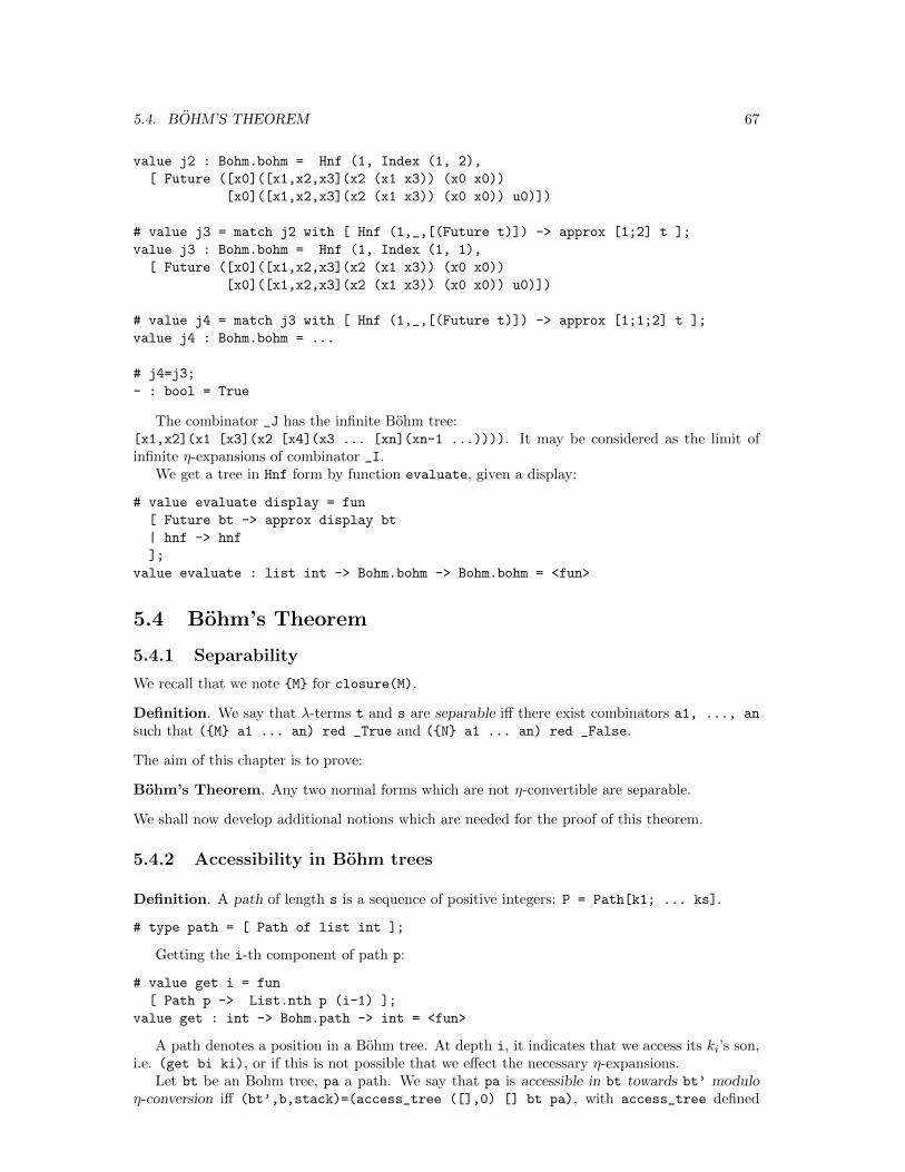
5.4. BOHM’S THEOREM 67
value j2 : Bohm.bohm = Hnf (1, Index (1, 2),
[ Future ([x0]([x1,x2,x3](x2 (x1 x3)) (x0 x0))
[x0]([x1,x2,x3](x2 (x1 x3)) (x0 x0)) u0)])
# value j3 = match j2 with [ Hnf (1,_,[(Future t)]) -> approx [1;2] t ];
value j3 : Bohm.bohm = Hnf (1, Index (1, 1),
[ Future ([x0]([x1,x2,x3](x2 (x1 x3)) (x0 x0))
[x0]([x1,x2,x3](x2 (x1 x3)) (x0 x0)) u0)])
# value j4 = match j3 with [ Hnf (1,_,[(Future t)]) -> approx [1;1;2] t ];
value j4 : Bohm.bohm = ...
# j4=j3;
- : bool = True
The combinator _J has the infinite Bohm tree:[x1,x2](x1 [x3](x2 [x4](x3 ... [xn](xn-1 ...)))). It may be considered as the limit ofinfinite η-expansions of combinator _I.
We get a tree in Hnf form by function evaluate, given a display:
# value evaluate display = fun
[ Future bt -> approx display bt
| hnf -> hnf
];
value evaluate : list int -> Bohm.bohm -> Bohm.bohm = <fun>
5.4 Bohm’s Theorem
5.4.1 Separability
We recall that we note {M} for closure(M).
Definition. We say that λ-terms t and s are separable iff there exist combinators a1, ..., an
such that ({M} a1 ... an) red _True and ({N} a1 ... an) red _False.
The aim of this chapter is to prove:
Bohm’s Theorem. Any two normal forms which are not η-convertible are separable.
We shall now develop additional notions which are needed for the proof of this theorem.
5.4.2 Accessibility in Bohm trees
Definition. A path of length s is a sequence of positive integers: P = Path[k1; ... ks].
# type path = [ Path of list int ];
Getting the i-th component of path p:
# value get i = fun
[ Path p -> List.nth p (i-1) ];
value get : int -> Bohm.path -> int = <fun>
A path denotes a position in a Bohm tree. At depth i, it indicates that we access its ki’s son,i.e. (get bi ki), or if this is not possible that we effect the necessary η-expansions.
Let bt be an Bohm tree, pa a path. We say that pa is accessible in bt towards bt’ moduloη-conversion iff (bt’,b,stack)=(access_tree ([],0) [] bt pa), with access_tree defined
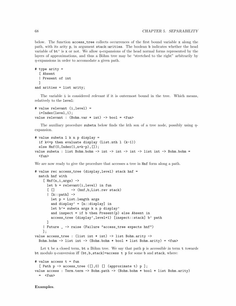
68 CHAPTER 5. SEPARABILITY
below. The function access_tree collects occurrences of the first bound variable x along thepath, with its arity p, in argument stack:arities. The boolean b indicates whether the headvariable of bt’ is x or not. We allow η-expansions of the head normal forms represented by thelayers of approximations, and thus a Bohm tree may be “stretched to the right” arbitrarily byη-expansions in order to accomodate a given path.
# type arity =
[ Absent
| Present of int
]
and arities = list arity;
The variable i is considered relevant if it is outermost bound in the tree. Which means,relatively to the level:
# value relevant (i,level) =
i=Index(level,1);
value relevant : (Bohm.var * int) -> bool = <fun>
The auxiliary procedure subeta below finds the kth son of a tree node, possibly using η-expansion.
# value subeta l k n p display =
if k<=p then evaluate display (List.nth l (k-1))
else Hnf(0,Index(1,n+k-p),[]);
value subeta : list Bohm.bohm -> int -> int -> int -> list int -> Bohm.bohm =
<fun>
We are now ready to give the procedure that accesses a tree in Hnf form along a path.
# value rec access_tree (display,level) stack hnf =
match hnf with
[ Hnf(n,i,args) ->
let b = relevant(i,level) in fun
[ [] -> (hnf,b,List.rev stack)
| [k::path] ->
let p = List.length args
and display’ = [n::display] in
let b’= subeta args k n p display’
and inspect = if b then Present(p) else Absent in
access_tree (display’,level+1) [inspect::stack] b’ path
]
| Future _ -> raise (Failure "access_tree expects hnf")
];
value access_tree : (list int * int) -> list Bohm.arity ->
Bohm.bohm -> list int -> (Bohm.bohm * bool * list Bohm.arity) = <fun>
Let t be a closed term, bt a Bohm tree. We say that path p is accessible in term t towardsbt modulo η-conversion iff (bt,b,stack)=access t p for some b and stack, where:
# value access t = fun
[ Path p -> access_tree ([],0) [] (approximate t) p ];
value access : Term.term -> Bohm.path -> (Bohm.bohm * bool * list Bohm.arity)
= <fun>
Examples.
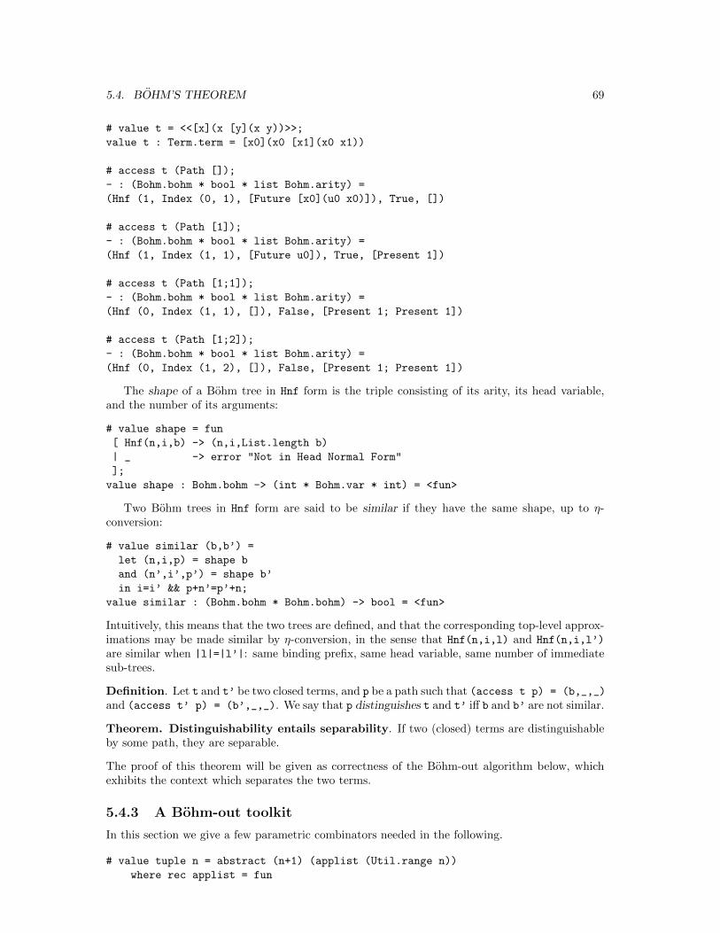
5.4. BOHM’S THEOREM 69
# value t = <<[x](x [y](x y))>>;
value t : Term.term = [x0](x0 [x1](x0 x1))
# access t (Path []);
- : (Bohm.bohm * bool * list Bohm.arity) =
(Hnf (1, Index (0, 1), [Future [x0](u0 x0)]), True, [])
# access t (Path [1]);
- : (Bohm.bohm * bool * list Bohm.arity) =
(Hnf (1, Index (1, 1), [Future u0]), True, [Present 1])
# access t (Path [1;1]);
- : (Bohm.bohm * bool * list Bohm.arity) =
(Hnf (0, Index (1, 1), []), False, [Present 1; Present 1])
# access t (Path [1;2]);
- : (Bohm.bohm * bool * list Bohm.arity) =
(Hnf (0, Index (1, 2), []), False, [Present 1; Present 1])
The shape of a Bohm tree in Hnf form is the triple consisting of its arity, its head variable,and the number of its arguments:
# value shape = fun
[ Hnf(n,i,b) -> (n,i,List.length b)
| _ -> error "Not in Head Normal Form"
];
value shape : Bohm.bohm -> (int * Bohm.var * int) = <fun>
Two Bohm trees in Hnf form are said to be similar if they have the same shape, up to η-conversion:
# value similar (b,b’) =
let (n,i,p) = shape b
and (n’,i’,p’) = shape b’
in i=i’ && p+n’=p’+n;
value similar : (Bohm.bohm * Bohm.bohm) -> bool = <fun>
Intuitively, this means that the two trees are defined, and that the corresponding top-level approx-imations may be made similar by η-conversion, in the sense that Hnf(n,i,l) and Hnf(n,i,l’)
are similar when |l|=|l’|: same binding prefix, same head variable, same number of immediatesub-trees.
Definition. Let t and t’ be two closed terms, and p be a path such that (access t p) = (b,_,_)
and (access t’ p) = (b’,_,_). We say that p distinguishes t and t’ iff b and b’ are not similar.
Theorem. Distinguishability entails separability. If two (closed) terms are distinguishableby some path, they are separable.
The proof of this theorem will be given as correctness of the Bohm-out algorithm below, whichexhibits the context which separates the two terms.
5.4.3 A Bohm-out toolkit
In this section we give a few parametric combinators needed in the following.
# value tuple n = abstract (n+1) (applist (Util.range n))
where rec applist = fun
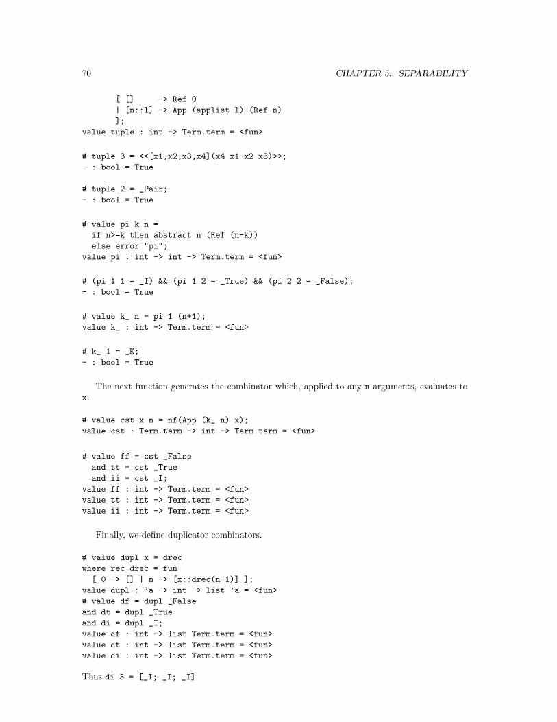
70 CHAPTER 5. SEPARABILITY
[ [] -> Ref 0
| [n::l] -> App (applist l) (Ref n)
];
value tuple : int -> Term.term = <fun>
# tuple 3 = <<[x1,x2,x3,x4](x4 x1 x2 x3)>>;
- : bool = True
# tuple 2 = _Pair;
- : bool = True
# value pi k n =
if n>=k then abstract n (Ref (n-k))
else error "pi";
value pi : int -> int -> Term.term = <fun>
# (pi 1 1 = _I) && (pi 1 2 = _True) && (pi 2 2 = _False);
- : bool = True
# value k_ n = pi 1 (n+1);
value k_ : int -> Term.term = <fun>
# k_ 1 = _K;
- : bool = True
The next function generates the combinator which, applied to any n arguments, evaluates tox.
# value cst x n = nf(App (k_ n) x);
value cst : Term.term -> int -> Term.term = <fun>
# value ff = cst _False
and tt = cst _True
and ii = cst _I;
value ff : int -> Term.term = <fun>
value tt : int -> Term.term = <fun>
value ii : int -> Term.term = <fun>
Finally, we define duplicator combinators.
# value dupl x = drec
where rec drec = fun
[ 0 -> [] | n -> [x::drec(n-1)] ];
value dupl : ’a -> int -> list ’a = <fun>
# value df = dupl _False
and dt = dupl _True
and di = dupl _I;
value df : int -> list Term.term = <fun>
value dt : int -> list Term.term = <fun>
value di : int -> list Term.term = <fun>
Thus di 3 = [_I; _I; _I].
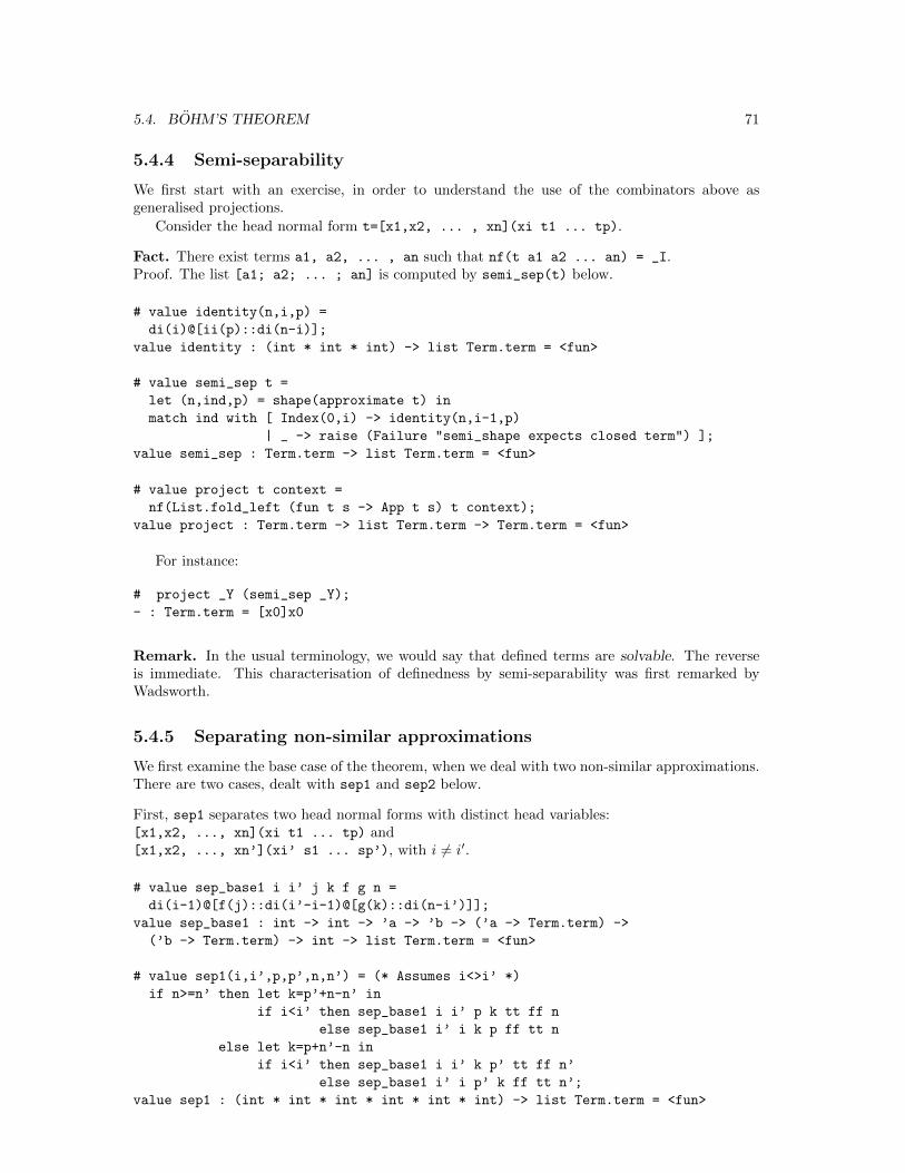
5.4. BOHM’S THEOREM 71
5.4.4 Semi-separability
We first start with an exercise, in order to understand the use of the combinators above asgeneralised projections.
Consider the head normal form t=[x1,x2, ... , xn](xi t1 ... tp).
Fact. There exist terms a1, a2, ... , an such that nf(t a1 a2 ... an) = _I.Proof. The list [a1; a2; ... ; an] is computed by semi_sep(t) below.
# value identity(n,i,p) =
di(i)@[ii(p)::di(n-i)];
value identity : (int * int * int) -> list Term.term = <fun>
# value semi_sep t =
let (n,ind,p) = shape(approximate t) in
match ind with [ Index(0,i) -> identity(n,i-1,p)
| _ -> raise (Failure "semi_shape expects closed term") ];
value semi_sep : Term.term -> list Term.term = <fun>
# value project t context =
nf(List.fold_left (fun t s -> App t s) t context);
value project : Term.term -> list Term.term -> Term.term = <fun>
For instance:
# project _Y (semi_sep _Y);
- : Term.term = [x0]x0
Remark. In the usual terminology, we would say that defined terms are solvable. The reverseis immediate. This characterisation of definedness by semi-separability was first remarked byWadsworth.
5.4.5 Separating non-similar approximations
We first examine the base case of the theorem, when we deal with two non-similar approximations.There are two cases, dealt with sep1 and sep2 below.
First, sep1 separates two head normal forms with distinct head variables:[x1,x2, ..., xn](xi t1 ... tp) and[x1,x2, ..., xn’](xi’ s1 ... sp’), with i 6= i′.
# value sep_base1 i i’ j k f g n =
di(i-1)@[f(j)::di(i’-i-1)@[g(k)::di(n-i’)]];
value sep_base1 : int -> int -> ’a -> ’b -> (’a -> Term.term) ->
(’b -> Term.term) -> int -> list Term.term = <fun>
# value sep1(i,i’,p,p’,n,n’) = (* Assumes i<>i’ *)
if n>=n’ then let k=p’+n-n’ in
if i<i’ then sep_base1 i i’ p k tt ff n
else sep_base1 i’ i k p ff tt n
else let k=p+n’-n in
if i<i’ then sep_base1 i i’ k p’ tt ff n’
else sep_base1 i’ i p’ k ff tt n’;
value sep1 : (int * int * int * int * int * int) -> list Term.term = <fun>
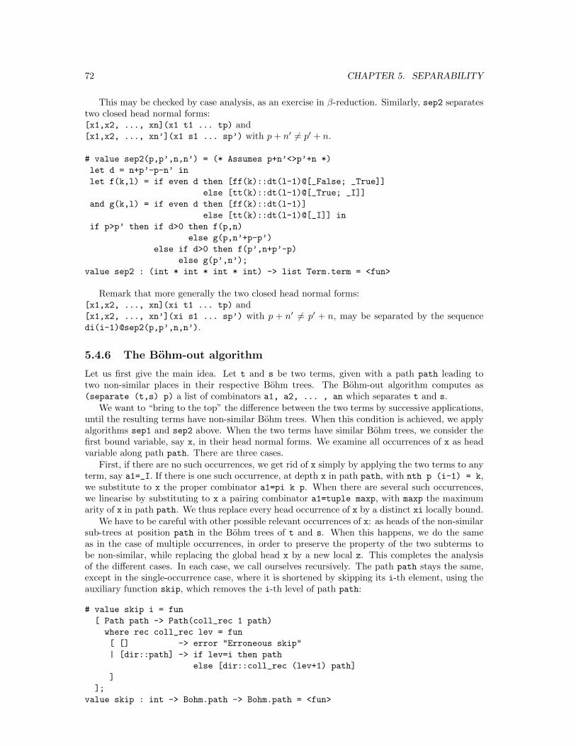
72 CHAPTER 5. SEPARABILITY
This may be checked by case analysis, as an exercise in β-reduction. Similarly, sep2 separatestwo closed head normal forms:[x1,x2, ..., xn](x1 t1 ... tp) and[x1,x2, ..., xn’](x1 s1 ... sp’) with p+ n′ 6= p′ + n.
# value sep2(p,p’,n,n’) = (* Assumes p+n’<>p’+n *)
let d = n+p’-p-n’ in
let f(k,l) = if even d then [ff(k)::dt(l-1)@[_False; _True]]
else [tt(k)::dt(l-1)@[_True; _I]]
and g(k,l) = if even d then [ff(k)::dt(l-1)]
else [tt(k)::dt(l-1)@[_I]] in
if p>p’ then if d>0 then f(p,n)
else g(p,n’+p-p’)
else if d>0 then f(p’,n+p’-p)
else g(p’,n’);
value sep2 : (int * int * int * int) -> list Term.term = <fun>
Remark that more generally the two closed head normal forms:[x1,x2, ..., xn](xi t1 ... tp) and[x1,x2, ..., xn’](xi s1 ... sp’) with p + n′ 6= p′ + n, may be separated by the sequencedi(i-1)@sep2(p,p’,n,n’).
5.4.6 The Bohm-out algorithm
Let us first give the main idea. Let t and s be two terms, given with a path path leading totwo non-similar places in their respective Bohm trees. The Bohm-out algorithm computes as(separate (t,s) p) a list of combinators a1, a2, ... , an which separates t and s.
We want to “bring to the top” the difference between the two terms by successive applications,until the resulting terms have non-similar Bohm trees. When this condition is achieved, we applyalgorithms sep1 and sep2 above. When the two terms have similar Bohm trees, we consider thefirst bound variable, say x, in their head normal forms. We examine all occurrences of x as headvariable along path path. There are three cases.
First, if there are no such occurrences, we get rid of x simply by applying the two terms to anyterm, say a1=_I. If there is one such occurrence, at depth x in path path, with nth p (i-1) = k,we substitute to x the proper combinator a1=pi k p. When there are several such occurrences,we linearise by substituting to x a pairing combinator a1=tuple maxp, with maxp the maximumarity of x in path path. We thus replace every head occurrence of x by a distinct xi locally bound.
We have to be careful with other possible relevant occurrences of x: as heads of the non-similarsub-trees at position path in the Bohm trees of t and s. When this happens, we do the sameas in the case of multiple occurrences, in order to preserve the property of the two subterms tobe non-similar, while replacing the global head x by a new local z. This completes the analysisof the different cases. In each case, we call ourselves recursively. The path path stays the same,except in the single-occurrence case, where it is shortened by skipping its i-th element, using theauxiliary function skip, which removes the i-th level of path path:
# value skip i = fun
[ Path path -> Path(coll_rec 1 path)
where rec coll_rec lev = fun
[ [] -> error "Erroneous skip"
| [dir::path] -> if lev=i then path
else [dir::coll_rec (lev+1) path]
]
];
value skip : int -> Bohm.path -> Bohm.path = <fun>
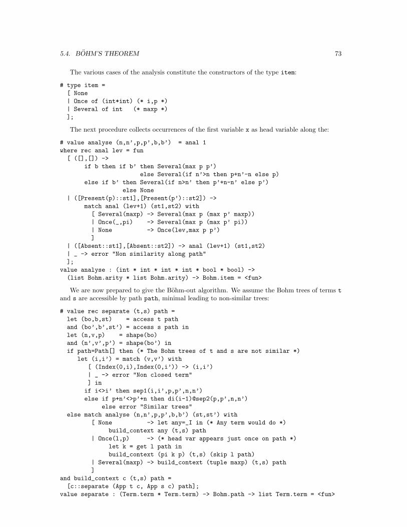
5.4. BOHM’S THEOREM 73
The various cases of the analysis constitute the constructors of the type item:
# type item =
[ None
| Once of (int*int) (* i,p *)
| Several of int (* maxp *)
];
The next procedure collects occurrences of the first variable x as head variable along the:
# value analyse (n,n’,p,p’,b,b’) = anal 1
where rec anal lev = fun
[ ([],[]) ->
if b then if b’ then Several(max p p’)
else Several(if n’>n then p+n’-n else p)
else if b’ then Several(if n>n’ then p’+n-n’ else p’)
else None
| ([Present(p)::st1],[Present(p’)::st2]) ->
match anal (lev+1) (st1,st2) with
[ Several(maxp) -> Several(max p (max p’ maxp))
| Once(_,pi) -> Several(max p (max p’ pi))
| None -> Once(lev,max p p’)
]
| ([Absent::st1],[Absent::st2]) -> anal (lev+1) (st1,st2)
| _ -> error "Non similarity along path"
];
value analyse : (int * int * int * int * bool * bool) ->
(list Bohm.arity * list Bohm.arity) -> Bohm.item = <fun>
We are now prepared to give the Bohm-out algorithm. We assume the Bohm trees of terms t
and s are accessible by path path, minimal leading to non-similar trees:
# value rec separate (t,s) path =
let (bo,b,st) = access t path
and (bo’,b’,st’) = access s path in
let (n,v,p) = shape(bo)
and (n’,v’,p’) = shape(bo’) in
if path=Path[] then (* The Bohm trees of t and s are not similar *)
let (i,i’) = match (v,v’) with
[ (Index(0,i),Index(0,i’)) -> (i,i’)
| _ -> error "Non closed term"
] in
if i<>i’ then sep1(i,i’,p,p’,n,n’)
else if p+n’<>p’+n then di(i-1)@sep2(p,p’,n,n’)
else error "Similar trees"
else match analyse (n,n’,p,p’,b,b’) (st,st’) with
[ None -> let any=_I in (* Any term would do *)
build_context any (t,s) path
| Once(l,p) -> (* head var appears just once on path *)
let k = get l path in
build_context (pi k p) (t,s) (skip l path)
| Several(maxp) -> build_context (tuple maxp) (t,s) path
]
and build_context c (t,s) path =
[c::separate (App t c, App s c) path];
value separate : (Term.term * Term.term) -> Bohm.path -> list Term.term = <fun>
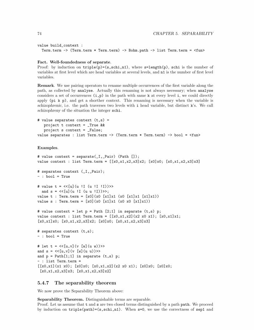
74 CHAPTER 5. SEPARABILITY
value build_context :
Term.term -> (Term.term * Term.term) -> Bohm.path -> list Term.term = <fun>
Fact. Well-foundedness of separate.Proof: by induction on triple(p)=(s,schi,n1), where s=length(p), schi is the number ofvariables at first level which are head variables at several levels, and n1 is the number of first levelvariables.
Remark. We use pairing operators to rename multiple occurrences of the first variable along thepath, as collected by analyse. Actually this renaming is not always necessary; when analyse
considers a set of occurrences (i,p) in the path with same k at every level i, we could directlyapply (pi k p), and get a shorther context. This renaming is necessary when the variable isschizophrenic, i.e. the path traverses two levels with i head variable, but distinct k’s. We callschizophreny of the situation the integer schi.
# value separates context (t,s) =
project t context = _True &&
project s context = _False;
value separates : list Term.term -> (Term.term * Term.term) -> bool = <fun>
Examples.
# value context = separate(_I,_Pair) (Path []);
value context : list Term.term = [[x0,x1,x2,x3]x2; [x0]x0; [x0,x1,x2,x3]x3]
# separates context (_I,_Pair);
- : bool = True
# value t = <<[u](u !I (u !I !I))>>
and s = <<[u](u !I (u u !I))>>;
value t : Term.term = [x0](x0 [x1]x1 (x0 [x1]x1 [x1]x1))
value s : Term.term = [x0](x0 [x1]x1 (x0 x0 [x1]x1))
# value context = let p = Path [2;1] in separate (t,s) p;
value context : list Term.term = [[x0,x1,x2](x2 x0 x1); [x0,x1]x1;
[x0,x1]x0; [x0,x1,x2,x3]x2; [x0]x0; [x0,x1,x2,x3]x3]
# separates context (t,s);
- : bool = True
# let t = <<[u,v](v [w](u w))>>
and s = <<[u,v](v [w](u u))>>
and p = Path[1;1] in separate (t,s) p;
- : list Term.term =
[[x0,x1](x1 x0); [x0]x0; [x0,x1,x2](x2 x0 x1); [x0]x0; [x0]x0;
[x0,x1,x2,x3]x3; [x0,x1,x2,x3]x2]
5.4.7 The separability theorem
We now prove the Separability Theorem above:
Separability Theorem. Distinguishable terms are separable.Proof. Let us assume that t and s are two closed terms distinguished by a path path. We proceedby induction on triple(path)=(s,schi,n1). When s=0, we use the correctness of sep1 and
5.4. BOHM’S THEOREM 75
sep2, a mere exercise in β-reduction. When s>0, we reason by cases on the number of times theoutermost bound variable x1 in the head normal forms of t and s occurs as head variable alongpath path. If it occurs just once at level m with arity p, and path goes through its k-th subtree,then (pi k p), applied to respectively t and s, will propagate by successive approximations intotheir respective Bohm trees until level m, which it will collapse in such a way that (skip m path),of length s-1, is a distinguishing path for them. The result follows by induction. It it occurs severaltimes, with maxp its maximum arity along P, we linearise x1 by substituting a1=tuple maxp toit. We check that path distinguishes (t a1) and (s a1), with decreased schizophreny schi-1.Finally, when it does not occur, we just eliminate x1 by substituting _I to it. We check that pathdistinguishes (t _I) and (s _I), with same schizophreny and n1-1 outermost bound variables.As remarked above, we treat the case where x1 appears as head variable of the tree accessed bypath in t or s in the same way as a multiple occurrence (see the base case of analyse above).This simplifies the treatment, since it defers the substitution to these head variables to the endof the Bohm-out process, with path empty. This may create a separating context longer thannecessary, but as remarked above we do not care here about minimizing the number of ai’s.
5.4.8 Searching for a separating path
In this section we shall attempt to find a path separating two λ-terms. This is not decidable ingeneral, and thus we can only hope for a semi-decision algorithm. The second difficulty is thechoice of a sub-tree in such a way that we avoid undefined sub-trees. We ignore this problem hereand thus look in the Bohm trees of the two terms in a left-most outermost manner.
Searching for a path separating two trees. search_path searchs in a depth-first, left-to-rightmanner.
# value tryfind f = findrec
where rec findrec = fun
[ [] -> raise (Failure "Not separable")
| [x::l] -> try f x with [ Failure _ -> findrec l]
];
value tryfind : (’a -> ’b) -> list ’a -> ’b = <fun>
# value rec search_path trees (dis,dis’) path =
match trees with
[ (Hnf(n,_,l), Hnf(n’,_,l’)) ->
if similar(trees) then
let p = List.length l
and d = [n::dis]
and p’ = List.length l’
and d’ = [n’::dis’] in
let check k =
let hnf = subeta l k n p d
and hnf’ = subeta l’ k n’ p’ d’ in
search_path (hnf,hnf’) (d,d’) [k::path]
in tryfind check (Util.range (max p p’))
else List.rev(path)
| _ -> raise (Failure "search_path expects hnfs")
];
value search_path : (Bohm.bohm * Bohm.bohm) -> (list int * list int) ->
list int -> list int = <fun>
Note. Similarity does not depend on the display. Further we do not need to keep track ofη-expansions. This is an essential property of our representation of variables with constructorIndex.

76 CHAPTER 5. SEPARABILITY
Finding a path separating two terms.
# value separ_path (t,s) =
Path(search_path (approximate t, approximate s) ([],[]) []);
value separ_path : (Term.term * Term.term) -> Bohm.path = <fun>
This procedure may loop because it looks depth-first, like for instance insepar_path(<<[x](x !Omega x)>>,<<[x](x !Omega !I)>>), or because the two terms are notseparable, like for instance in separ_path(_Y,_Fix). For certain non-separable pairs of terms, itactually fails, like for instance:
# separ_path(_I,_A);
Exception: Failure "Not separable".
Exercises.1. Program a breadth-first version search_path_breadth of search_path, which will returna path separating two trees if it can be found in a breadth-first search left to right. Thussearch_path_breadth ought to succeed on the approximations of terms <<[x,y](x !Y x)>> and<<[x,y](x !Y y)>>.2. The preceding procedure will still fail to find a path separating <<[x,y](x !Omega x)>> and<<[x,y](x !Omega y)>>, because it avoids looping on infinite branches, but still loops trying tofind an approximation to undefined terms. Write a semi-decision procedure separ_path whichwill return a path separating two terms if there exists one at all. This procedure must dove-tailsingle-steps β-reductions from the two terms, without attempting to compute head-normal forms.It will still loop on pairs such as (_Y,_Y), of course.
Remark. Combinators which are η-convertible, such as _A and _I, are not separable. Combina-tors which have the same Bohm trees, such as _Y and _Fix, are not either. Note also that thecombinator _I is not separable from _J, even though their Bohm trees are different, and they arenot finitely η-convertible.
5.4.9 Left Bohm separator
Putting the two together, we get a left Bohm separator as:
# value bohm (t,s) = separate (t,s) (separ_path (t,s));
value bohm : (Term.term * Term.term) -> list Term.term = <fun>
For instance:
# bohm(_I,_Pair);
- : list Term.term = [[x0,x1,x2,x3]x2; [x0]x0; [x0,x1,x2,x3]x3]
# bohm(_Zero,_One);
- : list Term.term = [[x0,x1,x2]x2; [x0,x1]x0]
# bohm(_I,_Y);
- : list Term.term = [[x0,x1,x2]x1; [x0,x1]x0; [x0,x1]x0; [x0]x0]
# bohm(_Delta,<<[x,y](x y y)>>);
- : list Term.term =
[[x0,x1,x2](x2 x0 x1); [x0,x1,x2,x3](x3 x0 x1 x2); [x0,x1]x0; [x0]x0;
[x0]x0; [x0,x1,x2,x3,x4]x3; [x0,x1,x2,x3,x4]x4]
# bohm(<<[u](u !I (u !I !I))>>,<<[u](u !I (u u !I))>>);
- : list Term.term =
5.5. TO KNOW MORE 77
[[x0,x1,x2](x2 x0 x1); [x0,x1]x1; [x0,x1]x0; [x0,x1,x2,x3]x2; [x0]x0;
[x0,x1,x2,x3]x3]
# bohm(<<[u,v](v [w](u w))>>,<<[u,v](v [w](u u))>>);
- : list Term.term =
[[x0,x1](x1 x0); [x0]x0; [x0,x1,x2](x2 x0 x1); [x0]x0; [x0]x0;
[x0,x1,x2,x3]x3; [x0,x1,x2,x3]x2]
# bohm(<<[u](u (u u u) u)>>,<<[u](u (u u [u,v,w](w u v)) u)>>);
- : list Term.term =
[[x0,x1,x2,x3](x3 x0 x1 x2); [x0]x0; [x0,x1,x2]x0; [x0]x0; [x0,x1,x2]x1;
[x0]x0; [x0]x0; [x0,x1,x2,x3,x4]x4; [x0,x1,x2,x3,x4]x3]
Proposition. If t and s are two closed normal forms which are not η-convertible, they aredistinguishable.Proof. By induction on the maximum height of the (finite) Bohm trees of t and s.Let t=[x1,x2, ..., xn](xi t1 ... tp) and s=[x1,x2, ..., xn’](xi’ s1 ... sp’). If t
and s are not similar, the empty path distinguishes them. Otherwise, we must have i=i’, andp+n’=p’+n. Assume for instance n≥n’: n=n’+d. The term s is η-convertible to[x1,x2, ..., xn](xi s1 ... sp), taking s(p’+j)=u(n’+j) for 1 ≤j≤d. Since t and s arenot η-convertible, there must exist 1≤k≤p such that tk is not η-convertible to sk; by inductionhypothesis these two terms are distinguishable by some path p, and thus t and s are distinguishableby path [k::p].
Corollary 1. Bohm’s theorem.Proof. Remark that two terms are η-convertible if and only if their closure is. Apply the Separa-bility Theorem.
Corollary 2. If t and s are two closed normal forms which are not η-convertible, separ_path(t,s)succeeds and returns a path which distinguishes them.Proof. separ_path(t,s) terminates with the shortest path in lexicographic ordering which dis-tinguishes t and s.
Corollary 3. If t and s are two closed normal forms which are not η-convertible, bohm(t,s)terminates with a context c such that (project t c)=_True and (project s c)=_False. Whent and s are η-convertible, bohm(t,s) terminates with exception Failure "Not separable".
The original presentation of Bohm’s theorem appared in [2]. The present development appearedin [5]. Many extensions of Bohm’s theorem have been studied, for instance for the simultaneousseparation of n terms. The separability problem is a special case of solving equations in λ−calculus.
The importance of Bohm’s theorem is that it gives a very strong requirement for a structure tobe a model of λ-calculus. Two normalisable terms are identifiable in a non-trivial model only ifthey are βη-convertible. This fixes roughly the three degrees of freedom of a model with respectto the completely syntactical one of Bohm trees:
• It may be extensional (i.e. verify η, possibly identify _I and _J) or not
• It may identify more or less the non-solvable terms
• It may be more or less rich in non-definable points.
5.5 To know more
The standard reference on λ-calculus is Barendregt’s book [1]. A good introduction is the monog-raphy by Hindley and Seldin [4].

78 CHAPTER 5. SEPARABILITY
Bibliography
[1] Henk Barendregt. The Lambda Calculus: Its Syntax and Semantics. North Holland, 1984.
[2] C. Bohm. Alcune proprieta delle forme β-η-normali nel λ-k-calcolo. Technical report, Pubbli-cazioni dell’Istituto per le Applicazioni del Calcolo N. 696, Roma, 1968.
[3] N. G. de Bruijn. Lambda-calculus notation with nameless dummies, a tool for automaticformula manipulation, with application to the Church-Rosser theorem. Indag. Math., 34:381–392, 1972.
[4] J. R. Hindley and J. P. Seldin. Introduction to Combinators and λ-Calculus. CambridgeUniversity Press, 1986.
[5] Gerard Huet. An analysis of Bohm’s theorem. Theoretical Computer Science, 121:145–167,1993.
[6] Gerard Huet. Residual theory in λ-calculus: a formal development. J. Functional Programming,4,3:371–394, 1994.
79