
Constructing an ±-maximizing option trading strategy in a multi
106
Master’s thesis Applied Mathematics (Chair: Stochastic System and Signal Theory, Track: Financial Engineering) Faculty of Electrical Engineering, Mathematics and Computer Science (EEMCS) Constructing an α-maximizing option trading strategy in a multi- dimensional setting Peter Bosschaart (s0176761) Assessment Committee: Prof. Dr. A. Bagchi (UT/SST) Prof. Dr. P. Guasoni (DCU/Stokes) Dr. Ir. E.A. van Doorn (UT/HS) Dr. B. Roorda (UT/IEBIS) Supervisors: Prof. Dr. P. Guasoni (DCU/Stokes) Prof. Dr. A. Bagchi (UT/SST) October 5, 2013
Transcript of Constructing an ±-maximizing option trading strategy in a multi

Master’s thesis Applied Mathematics(Chair: Stochastic System and Signal Theory, Track: Financial Engineering)Faculty of Electrical Engineering, Mathematics and Computer Science (EEMCS)
Constructing an α-maximizingoption trading strategy in a multi-dimensional setting
Peter Bosschaart (s0176761)
Assessment Committee:Prof. Dr. A. Bagchi (UT/SST)Prof. Dr. P. Guasoni (DCU/Stokes)Dr. Ir. E.A. van Doorn (UT/HS)Dr. B. Roorda (UT/IEBIS)
Supervisors:Prof. Dr. P. Guasoni (DCU/Stokes)Prof. Dr. A. Bagchi (UT/SST)
October 5, 2013


Preface
Dear reader,
Thank you for taking interest in this thesis, which I have written as final project for myMaster’s in Applied Mathematics at the University of Twente. The research for this thesis wasconducted at the mathematics department of the Dublin City University, Ireland, under theprimary supervision of Professor P. Guasoni. I would like to use this moment to express mygratitude to the people who have supported me throughout this project.
First of all, I would like to thank Professor P. Guasoni for giving me the opportunity ofworking with him and inviting me at the Dublin City University, giving me the chance to goabroad for my studies. It was a pleasure to work with him and I really appreciate the way inwhich he has supervised me. I am grateful for the informal, but professional atmosphere heprovided and the way he always could find the time to meet with me to discuss the project.
Second, I want to thank Professor A. Bagchi for supervising me at the University of Twente,especially in the last phase of the project. I wish him all the best in his retirement.
Third, the people of the mathematics department of the Dublin City University, for welcom-ing me in Ireland and at the Dublin City University. It was a pleasure to work alongside thisgroup. I would especially like to thank Dipl.-Ing. Dr. Eberhard Mayerhofer, who I came toknow as a good friend, and who took the time to read the concept version of this thesis andprovided me with a lot of useful feedback to establish the final version. Also, I would like tothank Christopher Belak, MSc. for being a good friend and introducing me to the city Dublin,as well as for setting up the database structure for the Optionmetrics database and teachingme the basics of MySQL language.
Finally, I would like to thank all other people who provided me with feedback on the con-cept version of the thesis, who supported me in academic or in personal ways throughout theproject, and all my friends and family who visited me in Dublin during my time there, providingpleasant distractions during the weekends.
I have really enjoyed working on this project abroad and cherish the experience I havegained this way. I hope that you as reader can see this reflected in this thesis and enjoy whilstreading it.
i

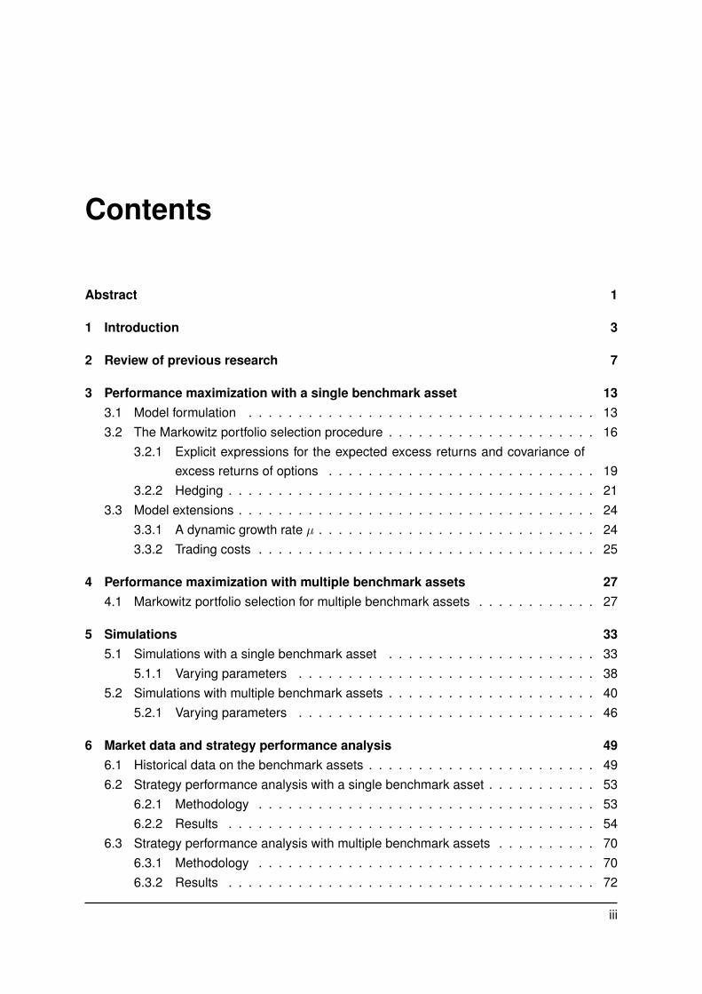
Contents
Abstract 1
1 Introduction 3
2 Review of previous research 7
3 Performance maximization with a single benchmark asset 133.1 Model formulation . . . . . . . . . . . . . . . . . . . . . . . . . . . . . . . . . . . 133.2 The Markowitz portfolio selection procedure . . . . . . . . . . . . . . . . . . . . . 16
3.2.1 Explicit expressions for the expected excess returns and covariance ofexcess returns of options . . . . . . . . . . . . . . . . . . . . . . . . . . . 19
3.2.2 Hedging . . . . . . . . . . . . . . . . . . . . . . . . . . . . . . . . . . . . . 213.3 Model extensions . . . . . . . . . . . . . . . . . . . . . . . . . . . . . . . . . . . . 24
3.3.1 A dynamic growth rate µ . . . . . . . . . . . . . . . . . . . . . . . . . . . . 243.3.2 Trading costs . . . . . . . . . . . . . . . . . . . . . . . . . . . . . . . . . . 25
4 Performance maximization with multiple benchmark assets 274.1 Markowitz portfolio selection for multiple benchmark assets . . . . . . . . . . . . 27
5 Simulations 335.1 Simulations with a single benchmark asset . . . . . . . . . . . . . . . . . . . . . 33
5.1.1 Varying parameters . . . . . . . . . . . . . . . . . . . . . . . . . . . . . . 385.2 Simulations with multiple benchmark assets . . . . . . . . . . . . . . . . . . . . . 40
5.2.1 Varying parameters . . . . . . . . . . . . . . . . . . . . . . . . . . . . . . 46
6 Market data and strategy performance analysis 496.1 Historical data on the benchmark assets . . . . . . . . . . . . . . . . . . . . . . . 496.2 Strategy performance analysis with a single benchmark asset . . . . . . . . . . . 53
6.2.1 Methodology . . . . . . . . . . . . . . . . . . . . . . . . . . . . . . . . . . 536.2.2 Results . . . . . . . . . . . . . . . . . . . . . . . . . . . . . . . . . . . . . 54
6.3 Strategy performance analysis with multiple benchmark assets . . . . . . . . . . 706.3.1 Methodology . . . . . . . . . . . . . . . . . . . . . . . . . . . . . . . . . . 706.3.2 Results . . . . . . . . . . . . . . . . . . . . . . . . . . . . . . . . . . . . . 72
iii

7 Conclusions and recommendations for further research 83
Bibliography I
A Proofs IIIA.1 Proof of Theorem 3.2.3 . . . . . . . . . . . . . . . . . . . . . . . . . . . . . . . . IIIA.2 Proof of Theorem 3.2.4 . . . . . . . . . . . . . . . . . . . . . . . . . . . . . . . . IVA.3 Proof of Theorem 4.1.1 . . . . . . . . . . . . . . . . . . . . . . . . . . . . . . . . V
B Tables IXB.1 Mean absolute portfolio weights . . . . . . . . . . . . . . . . . . . . . . . . . . . . IXB.2 Realized option excess returns analysis . . . . . . . . . . . . . . . . . . . . . . . XB.3 Expected option excess returns analysis . . . . . . . . . . . . . . . . . . . . . . . XII
iv

Abstract
In this thesis we derive a trading strategy which maximizes its excess returns, whilst control-ling for the standard deviation of these excess returns, by dynamically investing in a portfolio ofEuropean call options on one or multiple benchmark assets and the benchmarks themselves.We show that this implies that the Sharpe ratio of these excess returns is maximized and thatthis is equivalent to the maximization of Jensen’s alpha, the intercept in the ordinary leastsquares regression of these excess returns on the excess returns on the complete US equitymarket. The strategy is constructed such that the exposure of the obtained excess returns tothe excess returns on the complete US equity market is statistically insignificant. The portfolioselection procedure for this strategy turns out to be a variant of Markowitz portfolio selection,adapted to admit derivatives in the selection.
The strategy’s performance is studied in a theoretical framework, where the benchmarks followgeometric Brownian motions and options are priced at the benchmark’s volatility with the Black-Scholes formula. We find that in this setting it is hard to generate superior performance asthe statistical significance in the generated alphas is low. We also study the performance ofour strategy with historical market data on four major stock indices on the US equity marketover 1996-2013. In this setting we do find alphas that are significantly larger than zero andsubstantial Sharpe ratios, even in times of high volatility on the benchmarks, and that oneobtains even better results when considering more benchmarks to invest on.
1


CHAPTER 1
INTRODUCTION
A growing literature suggests that a hedge fund manager can generate a positive return on topof the risk free rate (an excess return) by following strategies that repeatedly invest in dynamicportfolios that consist of one or more options on an underlying asset and have the possibilityof holding the underlying asset itself. In previous research this has been shown through sim-ulations and examples, but it remains unclear about the magnitude of the excess returns thatcan be achieved and how big the involved risk is.
Coval and Shumway [1] state that under the Black-Scholes model assumptions, optionsare redundant assets, but when one deviates from these assumptions, one can generate sig-nificant option returns. Broadie et al. [2] agree and report high returns on-out-of-the money(OTM) puts and straddles on the S&P 500 and explain this by mispricing effects of the market.Eraker [3], Jones [4], Kapadia and Szado [5], Liang et al. [6] and Santa-Clara and Saretto [7]all report similar findings on a variety of underlying assets, however, not all of them control forthe involved risk. In these studies the term “risk” is used to denote the standard deviation ofachieved excess returns.
This thesis is a follow up research on Guasoni et al. [8], in which a theoretical answer isprovided for the questions that are left unanswered by the previous research. In this paper atrading strategy is derived which maximizes the alpha of the achieved excess returns, control-ling for the risk. This paper explains the achieved excess returns by a single factor ordinaryleast squares (OLS) regression:
rpf = α+ βrmkt + ε, (1.1)
where
• rpf is the vector of excess returns generated by the investment strategy,
• α is the regression intercept, which captures the amount of excess return that is gener-ated by the strategy itself (the excess returns linear projection orthogonal to the marketsexcess return), and is known as Jensen’s alpha,
• β is the sensitivity of the strategy excess returns with respect to the market excess re-turns,
• rmkt is the vector of excess returns on the market itself, making βrmkt the linear projectionof the strategy’s excess returns on the market excess returns,
3
CHAPTER 1. INTRODUCTION
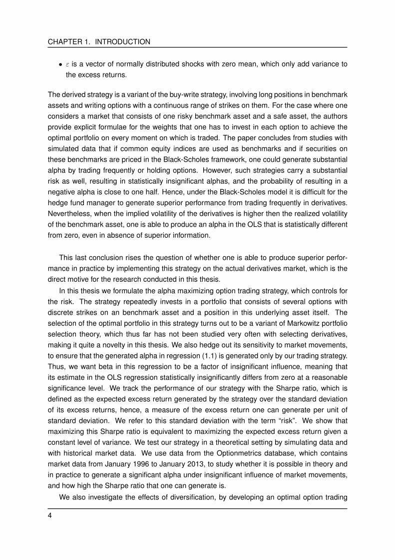
• ε is a vector of normally distributed shocks with zero mean, which only add variance tothe excess returns.
The derived strategy is a variant of the buy-write strategy, involving long positions in benchmarkassets and writing options with a continuous range of strikes on them. For the case where oneconsiders a market that consists of one risky benchmark asset and a safe asset, the authorsprovide explicit formulae for the weights that one has to invest in each option to achieve theoptimal portfolio on every moment on which is traded. The paper concludes from studies withsimulated data that if common equity indices are used as benchmarks and if securities onthese benchmarks are priced in the Black-Scholes framework, one could generate substantialalpha by trading frequently or holding options. However, such strategies carry a substantialrisk as well, resulting in statistically insignificant alphas, and the probability of resulting in anegative alpha is close to one half. Hence, under the Black-Scholes model it is difficult for thehedge fund manager to generate superior performance from trading frequently in derivatives.Nevertheless, when the implied volatility of the derivatives is higher then the realized volatilityof the benchmark asset, one is able to produce an alpha in the OLS that is statistically differentfrom zero, even in absence of superior information.
This last conclusion rises the question of whether one is able to produce superior perfor-mance in practice by implementing this strategy on the actual derivatives market, which is thedirect motive for the research conducted in this thesis.
In this thesis we formulate the alpha maximizing option trading strategy, which controls forthe risk. The strategy repeatedly invests in a portfolio that consists of several options withdiscrete strikes on an benchmark asset and a position in this underlying asset itself. Theselection of the optimal portfolio in this strategy turns out to be a variant of Markowitz portfolioselection theory, which thus far has not been studied very often with selecting derivatives,making it quite a novelty in this thesis. We also hedge out its sensitivity to market movements,to ensure that the generated alpha in regression (1.1) is generated only by our trading strategy.Thus, we want beta in this regression to be a factor of insignificant influence, meaning thatits estimate in the OLS regression statistically insignificantly differs from zero at a reasonablesignificance level. We track the performance of our strategy with the Sharpe ratio, which isdefined as the expected excess return generated by the strategy over the standard deviationof its excess returns, hence, a measure of the excess return one can generate per unit ofstandard deviation. We refer to this standard deviation with the term “risk”. We show thatmaximizing this Sharpe ratio is equivalent to maximizing the expected excess return given aconstant level of variance. We test our strategy in a theoretical setting by simulating data andwith historical market data. We use data from the Optionmetrics database, which containsmarket data from January 1996 to January 2013, to study whether it is possible in theory andin practice to generate a significant alpha under insignificant influence of market movements,and how high the Sharpe ratio that one can generate is.
We also investigate the effects of diversification, by developing an optimal option trading
4
CHAPTER 1. INTRODUCTION
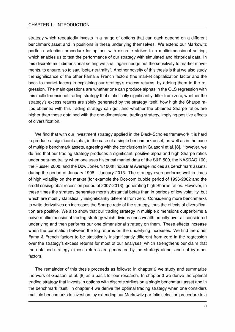
strategy which repeatedly invests in a range of options that can each depend on a differentbenchmark asset and in positions in these underlying themselves. We extend our Markowitzportfolio selection procedure for options with discrete strikes to a multidimensional setting,which enables us to test the performance of our strategy with simulated and historical data. Inthis discrete multidimensional setting we shall again hedge out the sensitivity to market move-ments, to ensure, so to say, “beta-neutrality”. Another novelty of this thesis is that we also studythe significance of the other Fama & French factors (the market capitalization factor and thebook-to-market factor) in explaining our strategy’s excess returns, by adding them to the re-gression. The main questions are whether one can produce alphas in the OLS regression withthis multidimensional trading strategy that statistically significantly differ from zero, whether thestrategy’s excess returns are solely generated by the strategy itself, how high the Sharpe ra-tios obtained with this trading strategy can get, and whether the obtained Sharpe ratios arehigher than those obtained with the one dimensional trading strategy, implying positive effectsof diversification.
We find that with our investment strategy applied in the Black-Scholes framework it is hardto produce a significant alpha, in the case of a single benchmark asset, as well as in the caseof multiple benchmark assets, agreeing with the conclusions in Guasoni et al. [8]. However, wedo find that our trading strategy produces a significant, positive alpha and high Sharpe ratiosunder beta-neutrality when one uses historical market data of the S&P 500, the NASDAQ 100,the Russell 2000, and the Dow Jones 1/100th Industrial Average indices as benchmark assets,during the period of January 1996 - January 2013. The strategy even performs well in timesof high volatility on the market (for example the Dot-com bubble period of 1996-2002 and thecredit crisis/global recession period of 2007-2013), generating high Sharpe ratios. However, inthese times the strategy generates more substantial betas than in periods of low volatility, butwhich are mostly statistically insignificantly different from zero. Considering more benchmarksto write derivatives on increases the Sharpe ratio of the strategy, thus the effects of diversifica-tion are positive. We also show that our trading strategy in multiple dimensions outperforms anaive multidimensional trading strategy which divides ones wealth equally over all consideredunderlying and then performs our one dimensional strategy on them. These effects increasewhen the correlation between the log returns on the underlying increases. We find the otherFama & French factors to be statistically insignificantly different from zero in the regressionover the strategy’s excess returns for most of our analyses, which strengthens our claim thatthe obtained strategy excess returns are generated by the strategy alone, and not by otherfactors.
The remainder of this thesis proceeds as follows: in chapter 2 we study and summarizethe work of Guasoni et al. [8] as a basis for our research. In chapter 3 we derive the optimaltrading strategy that invests in options with discrete strikes on a single benchmark asset and inthe benchmark itself. In chapter 4 we derive the optimal trading strategy when one considersmultiple benchmarks to invest on, by extending our Markowitz portfolio selection procedure to a
5

CHAPTER 1. INTRODUCTION
multidimensional setting. We then test our derived strategies with data simulated from a Black-Scholes framework in chapter 5. In chapter 6 we first present and analyze the historical marketdata from the Optionmetrics database which we use in our strategy performance analyses, andthen we test our strategies in a one and two dimensional setting, using different benchmarkassets during different sub-periods of 1996-2013. In chapter 7 we present our conclusions andwe make a few recommendations for further research.
6

CHAPTER 2
REVIEW OF PREVIOUS RESEARCH
This thesis is a follow up on Guasoni et al. [8]. In this chapter we introduce and summarizethe research presented in the paper “Performance maximization of actively managed funds”, inwhich the trading strategy is derived that trades in options with continuous strikes on a singlebenchmark asset and maximizes alpha in the regression (1.1), whilst controlling for the risk.The strategy turns out to be a variant of a buy-write strategy. Since this is a summary, theformulations in this chapter are sometimes very similar to the ones in the paper.
The motivation for the research conducted in this paper is that in previous literature it hasbeen reported that positive regression alphas can be obtained by frequently trading in options,but leaves it unclear what the magnitude of these alphas can be and how big the risk involvedis. A theoretical answer to these questions is derived in the paper, providing explicit formulaefor the trading strategy that maximizes alpha by trading frequently in options with continuousstrikes on a single benchmark, whilst controlling for the risk. In this thesis we bring the theoryderived in the paper to practice by formulating the strategy for options with discrete strikes andtesting the performance with historical market data. We also extend this strategy such that itcan trade in options with discrete strikes that can each depend on a different benchmark.
The paper states that a lot of different trading strategies from the previous literature pro-duce high alphas, but at a high level of risk, making the estimated alphas in the regressionover the returns statistically insignificantly different from zero, and the probability of generatinga negative alpha is close to one-half. Also, the question arises whether an investor could repli-cate the return generated by the strategy by investing in a set of benchmark assets. If not, howmuch more return can one generate with respect to the benchmark space? And what is theprobability of actually generating more, in stead of less, return with respect to the benchmarkspace? The difference between the generated return and the return that can be generated withthe benchmarks is labeled alpha, and is widely used in practice to measure the performanceof a fund. The standard error of alpha, which measures the uncertainty of alpha, is used asthe tracking error of the fund. The resulting ratio of alpha to its tracking error is referred to asthe appraisal ratio. A high appraisal ratio indicates superior performance, because it indicatesa high probability of a positive return. Maximizing this appraisal ratio is necessary for maxi-mizing the Sharpe ratio, which is a widely used measure of fund performance. For a hedgefund, the appraisal ratio of the fund is itself the Sharpe ratio of the hedged position that neutral-izes the benchmark risk. The appraisal ratio is the asymptotic T-statistic of the estimated alpha.
7
CHAPTER 2. REVIEW OF PREVIOUS RESEARCH
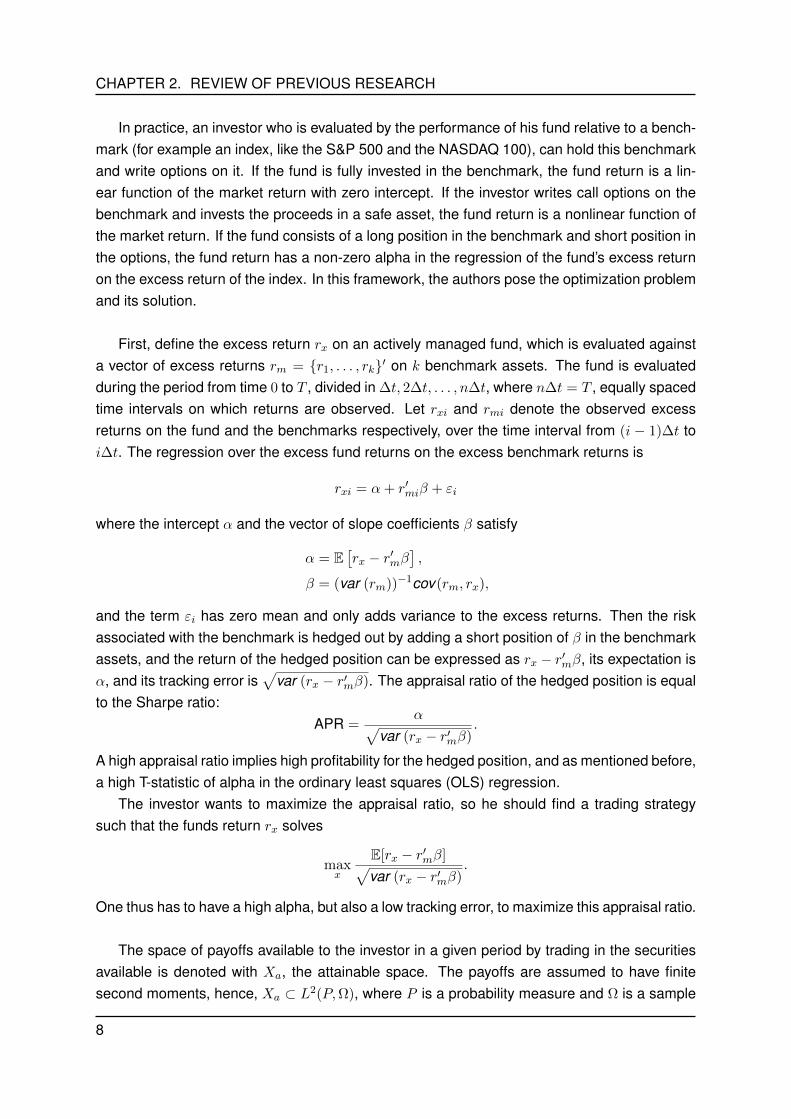
In practice, an investor who is evaluated by the performance of his fund relative to a bench-mark (for example an index, like the S&P 500 and the NASDAQ 100), can hold this benchmarkand write options on it. If the fund is fully invested in the benchmark, the fund return is a lin-ear function of the market return with zero intercept. If the investor writes call options on thebenchmark and invests the proceeds in a safe asset, the fund return is a nonlinear function ofthe market return. If the fund consists of a long position in the benchmark and short position inthe options, the fund return has a non-zero alpha in the regression of the fund’s excess returnon the excess return of the index. In this framework, the authors pose the optimization problemand its solution.
First, define the excess return rx on an actively managed fund, which is evaluated againsta vector of excess returns rm = r1, . . . , rk′ on k benchmark assets. The fund is evaluatedduring the period from time 0 to T , divided in ∆t, 2∆t, . . . , n∆t, where n∆t = T , equally spacedtime intervals on which returns are observed. Let rxi and rmi denote the observed excessreturns on the fund and the benchmarks respectively, over the time interval from (i − 1)∆t toi∆t. The regression over the excess fund returns on the excess benchmark returns is
rxi = α+ r′miβ + εi
where the intercept α and the vector of slope coefficients β satisfy
α = E[rx − r′mβ
],
β = (var (rm))−1cov(rm, rx),
and the term εi has zero mean and only adds variance to the excess returns. Then the riskassociated with the benchmark is hedged out by adding a short position of β in the benchmarkassets, and the return of the hedged position can be expressed as rx − r′mβ, its expectation isα, and its tracking error is
√var (rx − r′mβ). The appraisal ratio of the hedged position is equal
to the Sharpe ratio:APR =
α√var (rx − r′mβ)
.
A high appraisal ratio implies high profitability for the hedged position, and as mentioned before,a high T-statistic of alpha in the ordinary least squares (OLS) regression.
The investor wants to maximize the appraisal ratio, so he should find a trading strategysuch that the funds return rx solves
maxx
E[rx − r′mβ]√var (rx − r′mβ)
.
One thus has to have a high alpha, but also a low tracking error, to maximize this appraisal ratio.
The space of payoffs available to the investor in a given period by trading in the securitiesavailable is denoted with Xa, the attainable space. The payoffs are assumed to have finitesecond moments, hence, Xa ⊂ L2(P,Ω), where P is a probability measure and Ω is a sample
8
CHAPTER 2. REVIEW OF PREVIOUS RESEARCH
space, and L2(P,Ω) is the set of all measurable functions with finite second moments. Thenorm on this space is given by ||x|| = E[x2]1/2. The assumption of finite second moments isa minimal requirement to ensure that the sample estimates of linear regressions converge totheir population counterparts. The space Xa allows the market to be incomplete, because it isallowed to be a strict subset of L2(P,Ω). Its dimension could be infinite, which allows optionswith a continuous range of strikes and maturities on the benchmarks. The only constraint onthe linearity of the payoff space.
The linear space of payoffs spanned by the benchmark assets, is denoted by Xb and re-ferred to as the benchmark space. Its dimension is assumed to be k+1. Let xjj=0,...,k be thepayoffs of the k + 1 independent assets that span Xb. Let the first payoff, x0, be the constantpayoff of a safe asset. A fund has abnormal return relative to its benchmarks if, and only if, itsreturn or payoff falls outside the benchmark space. This can only be the case of Xb is a strictsubset of Xa.
Let ν : Xa 7→ < be the pricing function. Assume that the law of one price holds, thus ν islinear. Define a stochastic discount factor (SDF) for Xa as a random variable m ∈ L2(P,Ω)
such that ν(x) = E[xm] for all x ∈ Xa. Let Ma denote the set of all SDFs for Xa with Ma. Then,by Riesz representation theorem, the exists some ma ∈ Xa such that ν(x) = E[xma] for allx ∈ Xa, thus, ma ∈ Xa ∩Ma. It follows that ma is of smallest norm. The price function alsoapplies to the set of benchmark assets, so the set of SDFs for Xb is Mb = m ∈ L2(P,Ω) :
ν(x) = E[mx] for all x ∈ Xb, and there exists a smallest norm SDF mb ∈ Xb ∩Mb.
A trading strategy corresponds to a payoff x ∈ Xa. Assume that the payoff of the safe assetis x0 = 1 and that its price is ν(1) > 0. The return on the safe asset is thus R0 = 1/ν(1). Onecan then write the excess return on the fund as rx = x − ν(x)R0, and the excess return onthe j-th benchmark as rj = xj − ν(xj)R0 (for i = 1, . . . , k). Let rm = r1, . . . , rk′. Based onobservations (rx, r
′m) over n time intervals of equal length, one can obtain estimates of alpha
(denoted αn) and the appraisal ratio (denoted APRn) by the OLS regression. As n → ∞ theestimates converge to their population counterparts. The alpha and appraisal ratio depend onthe fund’s strategy x and are denoted with α(x) and APR(x).
The optimization problem translates to finding the strategy x that maximizes APR(x), de-noted by
APRmax = maxAPR(x) : x ∈ Xa.
The solution to this problem is found in a similar way as the construction of the mean-variancefrontier and is given by
Theorem 2.0.1. The alpha of any payoff x ∈ Xa is
α(x) = R0E[rx(mb −ma)].
The maximal appraisal ratio over all payoffs in Xa is
APRmax = R0||mb −ma||,
9
CHAPTER 2. REVIEW OF PREVIOUS RESEARCH
and the maximum is achieved for any payoff x of the form
x = z + θ(mb −ma)
for some z ∈ Xb and θ > 0.
Proof. For the proof of this theorem we refer the reader to Guasoni et al. [8].
The term mb −ma in the expression for the maximal appraisal ratio can be interpreted asthe Hansen and Jagannathan (HJ) distance from mb to the set of discount factors that price allpayoffs in Xa. The HJ distance is
δ = min||mb −m|| : m ∈Ma.
One can write any SDF m ∈Ma as m = ma + (m−ma) with E[(m−ma)x] = 0 for all x ∈ Xa.From mb −ma ∈ Xa follows that
||mb −m||2 = ||mb −ma||2 + ||m−ma||2,
and the minimum of ||mb −m|| over m ∈Ma is achieved when ||m−ma|| = 0, thus APRmax =
R0δ. The maximal appraisal ratio can be related to the variance bounds, known as the HansenJagannathan bounds; one can reduce the expression for the maximal appraisal ratio to
APRmax = R0
√var (ma)− var (mb),
and according to Hansen and Jagannathan, var (ma) is the greatest lower bound of the vari-ance of the SDFs in Ma, and the same statement holds for var (mb) and Mb. Furthermore, onecan write the Sharpe ratios of both spaces as
SHPi = R0
√var (mi), for i = a, b,
which implies
APRmax =
√SHP2
a − SHP2b .
Theorem 2.0.1 solves the maximization problem of the appraisal ratio and provides the so-lution of the maximization of alpha itself, but in practice there could be some constraints onthe maximization of alpha. The authors mention two constraints. One, the investor might notexceed a certain level of risk; typical risk management mandates that the tracking error of thestrategy is to be lower than a certain upper bound. Second, investors can face collateral re-quirements, which depend on the riskiness of the total position, that limit their leverage. Theauthors provide the explicit expressions for the maximal alpha in these cases as well.
The paper then studies maximal performance in a complete market; the implications ofTheorem 2.0.1 are studied under the assumption that the benchmark assets follow a geometricBrownian motion. An explicit solution for SHPb is easily derived from the moments of thebenchmark returns. An explicit solution for SHPa is harder to obtain, because Xa could contain
10
CHAPTER 2. REVIEW OF PREVIOUS RESEARCH
infinitely many security payoffs. If the market is complete, the space Xa = L2(P,Ω) and onecan obtain a minimum norm discount factorma in L2(P,Ω). Under the assumption of geometricBrownian motion price processes and a complete market an explicit expression for SHPa isderived. With these explicit expressions for the Sharpe ratios, an explicit expression for theappraisal ratio is obtained.
The derived formulae remain valid in the presence of additional securities other than thebenchmarks, which carry unpriced idiosyncratic risk. This means that using options on individ-ual securities cannot improve the appraisal ratio if the returns on the benchmark assets spanthe risk factors and the options on the benchmarks are used optimally.
To outperform the strategy of trading in benchmarks, the authors suggest to write optionson the benchmarks. They explore their intuition, by first applying Theorem 2.0.1 to describethe optimal option writing strategy and they argue that the relation between the pricing of theoptions and the process generating the benchmark returns is important for the assessment ofthe appraisal ratio that the optimal policy is likely to generate. The first case that is studied, isthe case where benchmarks follow geometric Brownian motion and options are priced accord-ing to the Black-Scholes formula, hence, physical and implied volatilities coincide. The authorsconsider a benchmark space of one risky asset in addition to the safe asset, in this case theexpression of the optimal payoff can be derived as a function of the benchmark return Rm.
Theorem 2.0.2. Assume that the benchmark space consists of only one risky asset and itsprice follows a geometric Brownian motion with growth rate µ and volatility σ. Assume thecontinuously compounded safe rate is r. Then, for any numbers γ and φ and any positivenumber θ, the payoff satisfies
x = γ + φRm − θf(Rm),
wheref(Rm) = cR−bm , with b = (µ− r)/σ2; c = e[−r+0.5b(µ+r−σ2)]∆t,
solves the optimization problem of the appraisal ratio.
Proof. For this proof we refer the reader to Guasoni et al. [8] again.
The payoff of the optimal strategy given in Theorem 2.0.2 is a nonlinear function of Rm,because f is nonlinear. The first derivative of f is negative (f ′ < 0) and the second derivativeof f is positive (f ′′ > 0). In the analysis of this strategy, the authors choose θ to be one,and φ in such a way that the delta of the strategy with respect to the benchmark is one. Theparameter γ is chosen so that the value of the strategy is one, to make x a return on a dollarinvestment. ∆t is set to one, so the returns are annualized. The authors then explain thatthe optimal strategy can be implemented by writing options on the benchmarks, because thenonlinear part of f(Rm) can be replicated by a portfolio of call and put options. Integration byparts shows that for any K > 0 and any twice differentiable function f , one has
f(Rm) = f(K) + f ′(K)(Rm −K) +
∫ K
0f ′′(k)(k −Rm)+ dk +
∫ ∞Kf ′′(k)(Rm − k)+ dk.
11

CHAPTER 2. REVIEW OF PREVIOUS RESEARCH
The first integration represents long positions in put options and the second integral representslong positions in call options. The second derivatives in these integrations give one the weightsone has to invest in options with strike k. Hence, the strategy works with a continuous rangeof strikes.
The authors test their strategy with simulated data in a Black-Scholes framework and con-clude that in this setting it is very hard to produce a statistically significant alpha. Then theyshow through simulation, that if one prices options at an implied volatility that is higher than therealized volatility, one is able to generate a significant alpha.
This last conclusion is the immediate motive for the research in this thesis. The authorshave performed their analysis with simulated options with higher implied volatilities than therealized volatilities on the benchmark. In our research, we derive an equivalent option tradingstrategy for options with discrete strikes and we then test this strategy with simulated andhistorical market data on traded options, for which the implied volatility generally differs fromthe realized volatility on the underlying. We also derive the equivalent strategy that considersmultiple benchmarks to invest on, which trades in options with discrete strikes that can eachdepend on a different, individual benchmark, and we test the performance of this strategy withsimulated and historical market data as well.
12
CHAPTER 3
PERFORMANCE MAXIMIZATION WITH A
SINGLE BENCHMARK ASSET
As we have elaborated on in chapter 2, Guasoni et al. [8] derive a performance maximizingoption trading strategy that repeatedly invests in a portfolio of options with continuous strikeson a single benchmark asset and a position in the underlying asset itself. However, such atheory could not be implemented in practice, as options are not available at every strike onthe derivatives market. In this chapter we derive an equivalent trading strategy that repeatedlyinvests in a portfolio of European call options with discrete strikes on a single benchmark assetand in this underlying itself. We show that this strategy maximizes alpha, controlling for therisk, and that this is equivalent to the maximization of the Sharpe ratio of excess returns.
We find that constructing a Markowitz portfolio of European call options with discrete strikesfor every trading period we consider maximizes the Sharpe ratio of the obtained excess returns.Dynamically investing in such a portfolio thus constitutes our trading strategy. The Markowitzportfolio selection procedure applied to derivatives in stead of equity securities is quite a noveltyof this thesis. After formulating our model for the dynamics of the benchmark price, the optionpricing framework and all involved assumptions, we therefore elaborate on why the Markowitzportfolio selection procedure meets our needs in maximizing the Sharpe ratio of the excessreturns that it generates and how it is adapted to support options in the selection procedure. Inthe remainder of this chapter we use our model and assumptions to derive explicit expressionsfor the expected excess returns on each option available on the moment on which we decideto trade and the covariance matrix of these excess returns, which are vital components in theconstruction of portfolio weights. We show how to adjust the weights such that beta-neutralityis ensured, and we formulate the performance maximizing portfolio weights for each momenton which we trade in explicit expressions. Finally, we pose two extensions to our model thatcould make the model more realistic.
3.1 Model formulation
Throughout this whole thesis, we assume that the price of the underlying (or, benchmark) assetfollows a geometric Brownian motion. The price process is given by:
dSt = µStdt+ σStdWt, (3.1)
13

CHAPTER 3. PERFORMANCE MAXIMIZATION WITH A SINGLE BENCHMARK ASSET
and is solved by
St = S0 · e(µ−σ2
2)t+σWt , (3.2)
in continuous time, where
• St is the price of the underlying at time t,
• S0 is the price of the underlying at time 0,
• µ is the growth rate of the Brownian motion,
• σ is the volatility of the Brownian motion,
• Wt is a standard Brownian motion.
The parameter µ is assumed to be constant, but one can extend the model in such a waythat this parameter does vary over time. We pose this model extension in section 3.3. Ina Black-Scholes framework, the parameter σ is also assumed to be constant, but when oneuses market data, one can use the historical/realized volatility process of the benchmark, whichmakes σ a time dependent variable. The assumption of a price process that follows a geomet-ric Brownian motion implies that the log returns of the underlying are normally distributed. Wejustify the use of a geometric Brownian motion process to model the underlying asset pricewith a few, straightforward arguments: first of all, a geometric Brownian motion only assumespositives values, which ensures us that the underlying price will not drop below zero. Second,the geometric Brownian motion generates the same kind of ‘random shocks’ in the asset price,which we also observe on the market, and last, the expected returns of a geometric Brownianmotion process are independent of the value of the process itself, which is also something thatagrees with the reality.
Now, define “trading days” as the dates on which we trade, i.e., as the days on which weassemble our portfolio of options. Let these trading days take place on t = 0,∆t, 2∆t, . . . ,
(k − 1)∆t (for certain integer k), between which are equally spaced time intervals ∆t. Nofurther action is undertaken on other days. The payoff of options depends on the price ofthe underlying at expiration of the options, which in this setting is observed in discrete time.Therefore, we rewrite the underlying price process in equation (3.2) in a discrete setting. Weassume that the options traded on trading day t have the same expiration date T = t+ ∆t. Wecan express the price of the underlying at expiration of the options traded on trading day t as:
ST = St · e(µ−σ2
2)∆t+σ
√∆tε, (3.3)
where
• ST is the price of the underlying at expiration of the options in our portfolio,
• St is the price of the underlying on trading day t,
14
CHAPTER 3. PERFORMANCE MAXIMIZATION WITH A SINGLE BENCHMARK ASSET
• ∆t = T − t is the time between the trading day and the time on which the options tradedon this trading day expire, denoted in annualized terms,
• ε is a standard normally distributed variable.
The portfolio assembled on trading day t will thus be evaluated at day T = t+ ∆t. The excessreturn on the benchmark during this period is given by
runderlyingt = e−rf (t)∆tSTSt− 1, (3.4)
where rf (t) is the annualized continuously compounded risk free interest rate on our tradingday t, which we henceforth abbreviate to rf , whilst noting it is still a function of time. In theBlack-Scholes model, rf is assumed to be constant over time.
Suppose that on a certain trading day t there are n− 1 European call options available onthe underlying, with strikes K1 > K2 > . . . > Kn−1 and corresponding prices C1, C2, . . . , Cn−1,and assume that all options have the same expiry. The price of these options under the riskneutral measure is given by EQ [e−rf∆t(ST −Ki)
+], for which an explicit expression is given
by the Black-Scholes formula:
Ci(St,∆t) = N(d1)St −N(d2)Kie−rf∆t, i = 1, 2, . . . , n− 1, (3.5)
with
d1 =1
σ√
∆t
[ln
(StKi
)+
(rf +
σ2
2
)∆t
], d2 = d1 − σ
√∆t, (3.6)
andN(x) =
1√2π
∫ x
−∞e−
12z2 dz,
the cumulative distribution function (CDF) of the standard normal distribution. The probabilitydensity function (PDF) of the standard normal distribution is given by
N ′(x) =1√2πe−
12x2 .
For hedging purposes we introduce a final, the n-th, option, which we shall refer to as the “zerostrike option”. With this option we facilitate a position in the underlying asset itself, hence thestrike of the option is zero and the price of the option is equal to the price of the underlying atour trading day, St. The realized excess return on each option is given by
ropti (t) =e−rf∆t(ST −Ki)
+
Ci− 1, i = 1, 2, . . . , n, (3.7)
and for the zero strike option, equation (3.7) reduces to equation (3.4). Let ropt1 (t), ropt2 (t), . . . ,
roptn (t)′ = rrealizedt ∈ <n×1 denote the vector containing the realized excess returns on alloptions available on this trading day t. We assume that the payoffs of all options have finitesecond moments, which is a minimal requirement to ensure that the sample estimates of linear
15
CHAPTER 3. PERFORMANCE MAXIMIZATION WITH A SINGLE BENCHMARK ASSET
regressions converge to their population counterparts.
When one uses market data, then one can observe the option prices Ci on the market andone can relax the Black-Scholes model assumptions for pricing the options. The fact that thereis a difference between the prices dictated by the market and the ones given by the Black-Scholes model is referred to as “market mispricing”.
We omit put options in our portfolio selection, for most of the put options on the market areof American exercising style, making the models more complicated. With the put-call parity
Pi(St,∆t) = Kie−rf∆t − St + Ci(St,∆t) (3.8)
one can synthesize European style puts, and we can interpret positions in certain calls as po-sitions in puts, cash and in the underlying.
Now that we have our model and options framework, we proceed with the issue of choos-ing the optimal portfolio on each trading day, which in this case is the portfolio with the highestexpected excess return for a given level of standard deviation in these excess returns. Weshall refer to the standard deviation of the obtained excess returns with the term “risk”, whichdeviates from more traditional formulations of risk, like the possibility of loss when a companydefaults and the Value at Risk. We define a unit of standard deviation as a unit of risk. As typi-cal risk management mandates that the tracking error of a strategy is to be lower than a certainupper bound, we construct the portfolio weights each trading day such that a predeterminedupper bound on the risk will not be crossed. This limits the magnitude of a negative excessreturn generated by the portfolio, and in such a way limits the potential of a ‘big’ loss, but it alsolimits our upward potential.
In the next section we show that the Markowitz portfolio selection procedure gives us theoptimal portfolio on each trading day and we derive explicit expressions for the figures neededin the assembly of this portfolio.
3.2 The Markowitz portfolio selection procedure
Our goal is to develop a trading strategy which maximizes our portfolios excess returns, con-trolling for the risk. Since the future is uncertain, we aim to maximize the expected portfolioexcess returns. We find that the Markowitz portfolio selection procedure does exactly this,though it is not common to use this theory with derivatives. Using this selection procedure withderivatives is quite a novelty, but has been performed before, for example by Liang et al. [6].We briefly introduce this selection procedure and its relevance for our research. We then de-rive the technicalities needed for our research.
16

CHAPTER 3. PERFORMANCE MAXIMIZATION WITH A SINGLE BENCHMARK ASSET
In 1952, Harry Markowitz [9] publishes the article “Portfolio selection”, which is still used asa basis in modern portfolio selection. He derives an asset selection procedure that maximizesthe discounted expected return of the portfolio, given a constant level of variance in these ex-cess returns, based on relevant beliefs of future performances of the assets which one canchoose from. He considers the discounted expected return, because the future is uncertain.The portfolio with maximum expected return is not necessarily the portfolio with minimum vari-ance, so one is able to pick a portfolio with a very high expected return, but bearing a very highvariance as well, which makes it an undesirable portfolio, that is why he seeks to maximize theexpected return, given the risk preference of the investor.
So, this selection procedure is highly suitable to fit our goals, but there are two issues. First,the Markowitz selection procedure as presented in the paper of Markowitz considers a rangeof different assets to assemble ones portfolio with, not derivatives on these assets. We wantto assemble a portfolio of European call options on one underlying asset, so we have to adaptthe portfolio selection procedure to this setting. Second, the selection procedure in the paperis presented in a static setting, meaning that the investor assembles his portfolio on one pointin time and then holds it. We want to develop a strategy that dynamically invests in a portfolioof options during a certain period, so selecting a portfolio of options once and holding thisportfolio throughout this period does not yield the result we are aiming at.
We tackle this first issue by treating each available option on a trading day as if it werean asset available in the Markowitz portfolio selection procedure. In this setting, one is ableto follow the same derivations as in Markowitz [9], but with somewhat different expressions,accounting for the fact that options have a different payoff than the underlying. The secondissue is fairly easy to tackle; on each trading day we assemble our portfolio in a static setting,knowing exactly when the options expire and thus, when an excess return is generated on theportfolio. After all options have expired, the portfolio is useless and is thus dissolved. Assem-bling a Markowitz portfolio on each trading day with the available European call options on thattrading day constitutes our dynamic trading strategy that maximizes alpha, and controls for therisk.
We first formulate the framework in which we are going to work for our portfolio selection oneach trading day, and then we show in Proposition 3.2.1 that the Markowitz portfolio selectionprocedure also gives us the maximal Sharpe ratio. Maximizing the Sharpe ratio of every port-folio we assemble, maximizes the Sharpe ratio of all excess returns obtained with our strategy,and thus alpha in our regression (1.1). We then derive explicit expressions for the terms usedin the Markowitz portfolio selection procedure on each trading day and extend the selectionprocedure with hedging arguments that will lead to beta-neutrality of the excess returns.
Consider a certain trading day t. On this day we invest in a range of options, including thezero strike option, hence in the underlying itself. Let πi(t) denote the weight (the proportion ofour wealth) of the option with strike Ki we buy (when πi > 0) in our portfolio or short (whenπi < 0) on this trading day. We directly drop the time index to abbreviate to πi for practical
17
CHAPTER 3. PERFORMANCE MAXIMIZATION WITH A SINGLE BENCHMARK ASSET
reasons. Let π1, π2, . . . , πn′ = π ∈ <n×1 denote the vector that contains all these weights.In equation (3.7) the realized excess return for each option is given, hence, we can write therealized excess return of our portfolio under choice of π as Rπ =
∑ni=1 πi · r
opti (t) = π′rrealizedt
(for which we also omit the time index). Its variance is denoted with var (Rπ), and its standarddeviation with σ(Rπ). The Sharpe ratio of the excess return generated by our portfolio choiceon this trading day is now given by E[Rπ]/σ(Rπ). We formalize our claim that the Markowitzselection procedure maximizes the Sharpe ratio of excess returns in Proposition 3.2.1. Thefirst two formulations in Proposition 3.2.1 are the formulations from which Markowitz derivedhis selection procedure, using Rπ as the vector of excess returns generated by the differentassets in the portfolio under the choice of weights π.
Proposition 3.2.1. The following statements are equivalent:
(i) maxπE[Rπ] : var (Rπ) = σ2,
(ii) minπvar (Rπ) : E[Rπ] = µ,
(iii) maxπE[Rπ]/σ(Rπ).
Proof. Equivalence of the first two statements follows easily from introducing Lagrange multi-pliers and the fact that maximizing an expression f is the same as minimizing −f . Equivalenceof the first two statements and the third follows from the fact that the first two statements finda point on the mean-variance frontier, which’ slope is exactly the Sharpe ratio, as is argued inCochrane [10].
So, using the Markowitz procedure to select our derivatives every trading day, we maximizethe Sharpe ratio of our excess return generated by the portfolio. To choose our weights opti-mally on such a trading day, we follow the same derivations as Markowitz [9], but adapt themto options. In the selection procedure the vector of expected excess returns on the assetsand the covariance matrix between them are used in the construction of the portfolio weights.We introduce mi(t) = E[ropti (t)], the expected excess return on an option with strike Ki tradedon trading day t, m(t) = m1(t),m2(t), . . . ,mn(t)′ ∈ <n×1, the vector containing all theseexpected excess returns, which we shall abbreviate to m, and we introduce S ∈ <n×n, thecovariance matrix of option excess returns, omitting its time index as well. Now we can write
E[Rπ] = π′m, var (Rπ) = π′Sπ,
and we arrive at the following Lemma that gives us the optimal portfolio weights on a certaintrading day when we do not incur any hedging.
Lemma 3.2.2. The weights π that maximize E[Rπ] : var (Rπ) = σ2 and the Sharpe ratio ofexcess returns on a certain trading day are given by
π = λS−1m,
with λ = σ/√m′S−1m,
(3.9)
18
CHAPTER 3. PERFORMANCE MAXIMIZATION WITH A SINGLE BENCHMARK ASSET
where m is the vector of expected excess returns on all options available on that trading day,and S is the covariance matrix of these excess returns.
Proof. We take the first statement from Proposition 3.2.1 and we introduce the Lagrange mul-tiplier γ/2:
maxπE[Rπ] : var (Rπ) = σ2 ⇔ max
π,γE[Rπ]− γ
2var (Rπ) = max
π,γπ′m− γ
2π′Sπ.
When we take the derivative of the target function w.r.t. π and set the equation equal to zero,we get
m− γSπ = 0⇒ π =1
γS−1m.
Now, setting λ = 1/γ, we get the first equality in equation (3.9). Finally, we need to meetthe variance restriction var (Rπ) = σ2 by choosing λ correctly. We plug π into the varianceexpression:
var (Rπ) = π′Sπ = (λS−1m)′S(λS−1m) = λ2π′Sπ = σ2, with π = S−1m
⇒ λ = σ/√π′Sπ = σ/
√(S−1m)′S(S−1m) = σ/
√m′S−1m,
and we arrive at the result.
With these weights we optimize our expected excess returns, adjusted for the risk σ. Wecan adjust λ in the weights to match our risk preference of σ per trading period. If one were touse these weights in practice, one needs expressions for m and S, which we derive in the nextsubsection. Furthermore, we want to hedge out our β-position w.r.t. the market, so we have toadjust the weights derived in Lemma 3.2.2 some more. This is elaborated on in section 3.2.2.
3.2.1 Explicit expressions for the expected excess returns and covariance ofexcess returns of options
As our portfolio selection each trading day depends on the expected excess returns vectorm and the covariance matrix of excess returns S of that trading day, we need to find explicitexpressions for these quantities. We first focus on the vector m.
The expected option excess return vector m
We have that m = m1,m2, . . . ,mn′, and mi, i = 1, . . . , n is the expected excess returnthat is generated by an option with strike Ki:
mi = E[ropti ] = E[e−rf∆t(ST −Ki)
+
Ci− 1
]=e−rf∆tEP [(ST −Ki)
+]Ci
− 1, (3.10)
where rf ,Ki and Ci can be observed on the market, or where Ci is given under the riskneutral measure Q by the Black-Scholes model. Since we assume that the underlying followsa geometric Brownian motion, we can derive an explicit expression for the expected payoff ofthe option under the physical measure P, hence, one can express mi explicitly:
19

CHAPTER 3. PERFORMANCE MAXIMIZATION WITH A SINGLE BENCHMARK ASSET
Theorem 3.2.3. We can express the expected excess return of an European call option withstrike Ki and price Ci, i ∈ 1, 2, . . . , n, longed on trading day t and with expiration on T =
t+ ∆t, explicitly as
mi =e−rf∆t
[St · eµ∆tN(d2)−KiN(d1)
]Ci
− 1, (3.11)
where
d1 =ln [St/Ki] +
(µ− σ2
2
)∆t
σ√
∆t, d2 = d1 + σ
√∆t =
ln [St/Ki] +(µ+ σ2
2
)∆t
σ√
∆t.
Proof. For the proof of this theorem we refer the reader to Appendix A.1.
Now, one can assemble the vector m by calculating all mi individually. For the zero strikeoption one has that N(d2) = N(∞) = 1, which reduces equation (3.11) to
mn = E[roptn ] = e(µ−rf )∆t − 1, (3.12)
which is exactly the result we would expect, as it is the discounted expectation of a geometricBrownian motion return.
The covariance matrix of option excess returns S
The covariance matrix of option excess returns S has the following structure:
S =
cov
(ropt1 , ropt1
)cov
(ropt1 , ropt2
)· · · cov
(ropt1 , roptn
)cov
(ropt2 , ropt1
)cov
(ropt2 , ropt2
)· · · cov
(ropt2 , roptn
)...
.... . .
...
cov(roptn , ropt1
)cov
(roptn , ropt2
)· · · cov
(roptn , roptn
)
. (3.13)
We derive an explicit expression for the general term, cov(ropti , roptj
), i, j ∈ 1, 2, . . . , n, in
this matrix:
Theorem 3.2.4. We can express the covariance between the excess returns on European calloptions with strikes Ki and Kj , with corresponding prices Ci and Cj , i, j ∈ 1, 2, . . . , n, longedon trading day t and with expiration on T = t+ ∆t, explicitly as
cov(ropti , roptj
)=e−2rf∆t
CiCj
[S2t e
(2µ+σ2)∆tN(d3)− St(Ki +Kj)eµ∆tN(d4) +KiKjN(d5)
]− (mi + 1)(mj + 1),
(3.14)
20
CHAPTER 3. PERFORMANCE MAXIMIZATION WITH A SINGLE BENCHMARK ASSET
where
d3 =ln[St/max(Ki,Kj)] +
(µ+ 3σ2
2
)∆t
σ√
∆t,
d4 =ln[St/max(Ki,Kj)] +
(µ+ σ2
2
)∆t
σ√
∆t,
d5 =ln[St/max(Ki,Kj)] +
(µ− σ2
2
)∆t
σ√
∆t.
Proof. For the proof of this theorem we refer the reader to Appendix A.2.
One can assemble the covariance matrix S by calculating each individual component. Forthe covariance of excess returns of zero strike options, we get that N(d3) = N(∞) = 1, whichreduces equation (3.14) to
cov(roptn , roptn ) = var(roptn
)= e2(µ−rf )∆t
(eσ
2∆t − 1), (3.15)
which is exactly the result we would expect, as it is the discounted variance of a geometricBrownian motion return.
Having explicit expressions for m and S, we can compute the optimal portfolio weights π atevery trading day. However, we still want our portfolio excess returns to be explained solely byour strategy and not by market movements, so, considering our regression (1.1), we want betato be zero, or at least statistically insignificantly different from zero. With the current choice ofweights, beta is very unlikely to be insignificantly different from zero, hence, we want to removethe sensitivity of our strategy excess returns w.r.t. market movements by altering our weights.We show how this is done in the next section.
3.2.2 Hedging
As we have mentioned in the previous section, we want our strategy excess returns to beexplained by our strategy alone and not by the excess returns on the market. Therefore, weneed to adjust our portfolio weights each trading day in such a way that beta in the regression(1.1) is statistically insignificantly different from zero at an acceptable level of significance. Weperform a hedge in our portfolio that will realize this, in a similar way as Guasoni et al. [8], asdescribed in chapter 2. In this case, with “hedging” we mean removing the portfolio’s sensitivitywith the respect to the excess returns on the whole market, deviating from standard definitionsof hedging that refer to removing the portfolios sensitivity with respect to its own underlying as-set. Also, in traditional ways, hedges are often established by adding products to the portfolio.We shall establish the hedge by altering the weight of the zero strike option in our portfolio.Removing the portfolio’s sensitivity with respect to the market excess returns on each tradingday will make beta in regression (1.1) an insignificant factor.
21
CHAPTER 3. PERFORMANCE MAXIMIZATION WITH A SINGLE BENCHMARK ASSET
A natural, first thought would be to perform a delta-hedge, which is fairly easy to implementand does not need the zero strike option as a hedging position. We perform the hedge on theweights before the risk adjustment takes place. Define initial, unadjusted portfolio weights asπ = S−1m. If one has computed these weights, one can compute the total delta position ofthe portfolio. The delta of each option, ∆i, is given by the N(d1) of the Black-Scholes equation(3.5). Let ∆ = ∆1,∆2, . . . ,∆n′ ∈ <n×1 be the vector that contains the delta of all options.Then the total delta position of the portfolio is given by π′∆ = ∆pf . To make this position zero,we add a constant c to each of the weights, the value of which is determined by
(π + c)′∆ = ∆pf + c ·∑i
∆i = 0,
⇒ c =−∆pf∑i ∆i
.
Rebalancing the weights with this constant and then adjusting for the risk in each trading pe-riod makes the strategy delta-neutral, meaning that its sensitivity to movements in the price ofits own underlying is hedged out. Unfortunately, this does not imply a zero or insignificant betawhen one uses large time intervals. For example, when one uses a monthly interval, then thismethod will not work. Therefore, we need another approach.
To make our strategy beta-neutral, we perform a direct beta-hedge, by rebalancing theweight of the zero strike option. The beta of an option is given by cov(ropti , rmktt )/var
(rmktt
)(see chapters 5 and 6 of Cochrane [10] on beta-representations), where rmktt is the excessreturn on the market over the period of assembling our portfolio and expiration of the optionsin it. Unfortunately, measuring the covariance between an option excess return and the marketexcess return is not that easy, as they do not depend on the same underlying. Therefore, weshall hedge with option betas w.r.t. their own underlying, which are defined as
βi =cov(ropti , roptn )
var(roptn
) . (3.16)
The beta of the zero strike option, βn, is by definition equal to one. The total beta position ofthe portfolio prior to hedging is given by βpf =
∑i πiβi and we aim to make it zero by adjusting
the weight on the zero strike option. Now, the question is how to relate the zero strike optionbeta to the market excess returns. If we assume that the zero strike option is just as sensitiveto its own underlying as it is to the market, then the total beta position of the portfolio is itssensitivity to the market and we can hedge it out by subtracting it from the weight of the zerostrike option. However, when the zero strike option is more sensitive to the market then to itsown underlying, we would get overcompensation effects when we simply extract the total betaposition from the weight on the zero strike option, or when it is less sensitive to the market thanto its own underlying, we would not hedge out the total position by simply subtracting it. In thiscase, we should scale the amount we subtract from the zero strike option to account for theseeffects. Define the “market beta” of the zero strike option, βmkt, as the sensitivity of the zero
22
CHAPTER 3. PERFORMANCE MAXIMIZATION WITH A SINGLE BENCHMARK ASSET
strike option to the market excess returns, given by the covariance of excess returns on theunderlying and the market divided by the variance of market excess returns. We have threeoptions for choosing this market beta:
1. Assume that the market beta of the zero strike option is equal to one (implying that thestrategy’s sensitivity to the excess returns on its own underlying is equal to the sensitivityto the excess returns on the complete market).
2. Calculate the market beta of the zero strike option using a certain period prior to our firsttrade and keep constant over time.
3. Calculate the market beta of the zero strike option dynamically, using the same period asin option 2 to calculate the market beta used for our first portfolio, but then add every newobservation of the strategy excess returns and the market excess returns to the vectorswe use to calculate this market beta, and calculate it again on each trading day.
The first option is by far the easiest one, as no extra work has to be done. The secondand third option demand extra calculations. The market beta of the zero strike option, βmkt,can be computed by taking the excess returns of the market and the underlying over a certainperiod prior to our first trade and then calculate the covariance between these excess returnsdivided by the variance of the market excess returns, which can be done once (option 2) orevery trading day (option 3).
To hedge, we subtract the portfolio beta position from the initial weight of the zero strikeoption. When using option 1, this can be done directly. Define b = 0, 0, . . . , 0, βpf′ ∈ <n×1,and then subtract this vector from the initial weights and then adjust for the risk. When onedoes not assume that the market beta of the zero strike option is one, one needs to divide b
by the calculated market beta first, to compensate for the fact that the beta position we hedgewith is not equal to one; when it is larger than one, we need to subtract a smaller proportionof the weight on the zero strike option, when it is smaller than one, we need to subtract moreto obtain beta-neutrality with respect to the market. This procedure makes the portfolio betaequal to zero each trading day, so we expect the beta of our realized excess returns to be closeto zero as well.
Theorem 3.2.5. On each trading day, the weights π that maximize E[Rπ] : var (Rπ) = σ2 andthe Sharpe ratio of excess returns for that trading day, whilst hedging out the portfolio’s marketexposure, are given by
π = λ(S−1m− b
),
with λ = σ/√m′S−1m,
b = 0, 0, . . . , 0, βpf/βmkt′,
βpf =∑
i πicov(ropti ,roptn )
var(roptn ),
π = S−1m,
(3.17)
23
CHAPTER 3. PERFORMANCE MAXIMIZATION WITH A SINGLE BENCHMARK ASSET
and the elements of m are given by Theorem 3.2.3 and the elements of S by Theorem 3.2.4,and where one can choose βmkt either equal to one or compute it from historical excess re-turns, as the covariance of the underlying excess returns and the market excess returns dividedby the variance of the market excess returns beforehand and use it as a constant, or update itdynamically when new information is obtained each trading day.
Proof. The proof of this theorem is analog to the proof of Lemma 3.2.2, but it adds the hedgingarguments provided in this section.
If one where to choose his portfolio weights every trading day according to Theorem 3.2.5,one would have an alpha-maximizing option trading strategy in one dimension that controls forthe risk and hedges out the sensitivity to market movements. This strategy also maximizes theSharpe ratio of the strategy’s excess returns, which under beta-neutrality is given by α/σ(rpf ).In chapter 5 we test the performance of this strategy with simulated data from a Black-Scholesframework, and then we test the performance of the strategy using historical market data inchapter 6. We investigate whether alpha is statistically significantly different from zero, whetherbeta is an insignificant factor in the regression (1.1) and how high the Sharpe ratio can get. Wewill also test our three options for choosing βmkt and see what the effects are on the strategyperformance.
Finally, we can extend our model in a few ways to meet more market properties. We shortlydiscuss two of them in the next section.
3.3 Model extensions
The model assumptions made in section 3.1 are fairly basic. In this section we propose twomodel extensions, which could make the model more realistic. First, we have assumed thatthe growth rate of the underlying geometric Brownian motion is constant throughout time. Thisis not entirely realistic, so we propose an extension that makes µ a time-dependent variable.Second, we have assumed that one can buy and sell options at the same price. In practice,this is not the case, because there are trading costs involved; there is a substantial bid-askspread on the options. We introduce this bid-ask spread in a simple manner to the model. Weomit a bid-ask spread on the underlying itself, as it is far more liquid than the derivatives writtenon it, hence, if there were a spread, then it would be marginal. We analyze the effects of theimplementation of these extensions with our market data analysis in chapter 6.
3.3.1 A dynamic growth rate µ
As mentioned before, µ is the growth rate of the geometric Brownian motion of the underlyingasset price. In the geometric Brownian motion, this term is assumed to be constant, but wecan argue that this term should be time-dependent. For example, if we would assemble ourportfolio at every first trading day of the month and we would do this for several years, then it
24

CHAPTER 3. PERFORMANCE MAXIMIZATION WITH A SINGLE BENCHMARK ASSET
would be a strong assumption that the growth rate stays the same over all these years. Wemake it time-dependent in the following way:
µ(t) = rf (t) +1
2σ(t), (3.18)
where µ(t) is the growth rate on trading day t, rf (t) is the annualized, continuously com-pounded risk free interest rate on trading day t and σ(t) is the historical/realized volatility of theunderlying on this day. The factor 1/2 is the average Sharpe ratio on the US equity market inpostwar data; 8% average excess return divided by 16% average volatility (all are annualizedfigures). Hence, in this way µ(t) is the risk free rate plus the expected excess return on dayt, making it the expected return on day t, which agrees with the definition of the parameter.The dynamic growth rate is easy to implement this way, because it only uses terms that werealready introduced to the model. A simple substitution will do.
3.3.2 Trading costs
In practice, there are no frictionless markets. Hence, the assumption that one can buy and selloptions at the same price is a strong one. We try to implement trading costs for options to themodel in a very simple way. As mentioned before, we omit trading costs on the underlying, asit is far more liquid than the derivatives written on it.
Introducing trading costs beforehand by defining a bid price and an ask price complicatesthe strategy, because the strategy assumes one price for buying and selling. An overly simpleway of introducing trading costs to our model, is to do it in hindsight, so we can at least studytheir impact on the strategy’s performance. If our strategy consistently buys options of a certainlevel of moneyness and sells options of another level of moneyness, then we can adjust theirprices by a certain factor beforehand; if one buys an option, one has to pay more than theamount of money one would get when selling the same option, so say, if there are tradingcosts of x percent of the option price, then we multiply the prices of the options we buy witha factor 1 + x and the options we sell with 1 − x. Then we run the data analysis again, and ifthe strategy still consistently buys or sells the same options, then we can say something aboutthe effects of the trading costs on the magnitude of the Sharpe ratio of the strategy’s excessreturns. However, if we observe that in this new setting one sells options which first we bought,and vice versa, then this approach produces erroneous results and is therefore useless.
25


CHAPTER 4
PERFORMANCE MAXIMIZATION WITH
MULTIPLE BENCHMARK ASSETS
In the previous chapter we have derived a trading strategy that dynamically invests in a portfolioof European call options on a single benchmark asset. In this chapter we raise the questionwhether we can increase alpha (and thus the Sharpe ratio) by constructing a strategy thatdynamically invests in a portfolio that consists of a range of European call options that caneach depend on a different underlying benchmark asset. If the returns of all underlying areindependent, one can add squared Sharpe ratios. When there is correlation, we still expectaddition effects, but to a lesser extent. We expect an increase in the strategy’s Sharpe ratiodue to diversification in the portfolio. In this chapter we derive the alpha-maximizing strategy,controlled for the risk, for this setting with multiple benchmarks, by extending our Markowitzportfolio selection procedure of the previous chapter to one that admits European call optionswith discrete strikes that can each depend on a different, individual benchmark.
4.1 Markowitz portfolio selection for multiple benchmark assets
In this section we extend the Markowitz portfolio selection procedure derived in the previouschapter such that it supports multiple underlying assets and options with discrete strikes onthem. By the same arguments as in section 3.2 and Proposition 3.2.1 we conclude that theMarkowitz portfolio selection procedure still provides us with the maximal Sharpe ratio for eachtrading day. Investing dynamically in such a portfolio constitutes our strategy and maximizesthe Sharpe ratio of its excess returns. We first pose our multidimensional model and then wederive new explicit expressions for the optimal portfolio weights on each trading day.
Suppose that we haveN benchmark assets on which options can be traded, which each fol-low a geometric Brownian motion price process S(i)
t , i = 1, 2, . . . , N , with parameters µ1, . . . , µN
and σ1, . . . , σN , which can be correlated in the Brownian motion terms with parameter ρij . Sup-pose that there is a annualized risk free rate rf on every trading day.
Suppose that on a certain trading day t, t ∈ 0,∆t, 2∆t, . . . , (k − 1)∆t, there are ni
European call options available on benchmark i, with strikes K(i)1 > K
(i)2 > . . . > K
(i)ni
and prices C(i)1 , C
(i)2 , . . . , C
(i)ni , where we again use the nthi option as a zero strike option for
hedging purposes. Assume that all options on all underlying have the same expiration dateT = t + ∆t. We again assume that the payoffs of all options have finite second moments.
27
CHAPTER 4. PERFORMANCE MAXIMIZATION WITH MULTIPLE BENCHMARK ASSETS
Denote the excess return on option with strike Kj on underlying i with r(i)j . Denote with
r(i) = r(i)1 , r
(i)2 , . . . , r
(i)ni ′ ∈ <ni×1 the vector of realized option excess returns on underly-
ing i for the options traded on this trading day. We use ropt = r(1), r(2), . . . , r(N)′ ∈ <∑ni×1
as the vector containing all realized excess return vectors of all underlying. As options onlydepend on the price of their own underlying at expiry, there does not change anything for thevectors of expected excess returns on the options. We denote with m(i) the vector of expectedexcess returns of the options on underlying i, with its elements defined as in theorem 3.2.3.We combine these vectors m(i) in vector m = m(1),m(2), . . . ,m(N)′ ∈ <
∑ni×1, the vector
that contains all expected excess returns on all options on all underlying. We can express thecovariance matrix of option excess returns as
S =
S11 S12 · · · S1N
S21 S22 · · · S2N
......
. . ....
SN1 SN2 · · · SNN
∈ <∑ni×
∑ni , (4.1)
where Sii for i = 1, . . . , N is given by Theorem 3.2.4 and where S′ji = Sij for i, j = 1, . . . , N .We are left with finding explicit expressions for the elements of Sij , the covariance matrix ofexcess returns of options on underlying i and options on underlying j, where i 6= j. We expresssuch a covariance matrix as
Sij =
cov(r
(i)1 , r
(j)1 ) cov(r
(i)1 , r
(j)2 ) · · · cov(r
(i)1 , r
(j)nj )
cov(r(i)2 , r
(j)1 ) cov(r
(i)2 , r
(j)2 ) · · · cov(r
(i)2 , r
(j)nj )
......
. . ....
cov(r(i)ni , r
(j)1 ) cov(r
(i)ni , r
(j)2 ) · · · cov(r
(i)ni , r
(j)nj )
. (4.2)
We want to have explicit expressions for its entries. To this end, we divide the matrix into threecategories:
1. Covariances of the type cov(r(i)k , r
(j)l ), for k = 1, . . . , ni − 1 and l = 1, . . . , nj − 1,
2. Covariances of the type cov(r(i)ni , r
(j)k ), for k = 1, . . . , nj − 1, and cov(r
(i)k , r
(j)nj ), for k =
1, . . . , ni − 1, which are equivalent,
3. Covariances of the type cov(r(i)ni , r
(j)nj ).
We will derive explicit expressions for each class when considering two benchmark assets asfollows. The N -dimensional case follows the same derivations, but adds some terms. Ex-tension is straightforward. The results for the two dimensional setting are presented in thefollowing theorem.
Theorem 4.1.1. For N = 2, consider the covariance matrix component S12 of option excessreturns as in (4.2) and its three types of covariances. An explicit expression for covariances of
28

CHAPTER 4. PERFORMANCE MAXIMIZATION WITH MULTIPLE BENCHMARK ASSETS
type 1 is given by
cov(r(1)i , r
(2)j ) =
e−2rf∆t
C(1)i C
(2)j
[S
(1)t S
(2)t e(µ1+µ2+ρ12σ1σ2)∆tMN(d1, d2)−K(1)
i S(2)t eµ2∆tMN(d3, d4)
−K(2)j S
(1)t eµ1∆tMN(d5, d6) +K
(1)i K
(2)j MN(d7, d8)
]− (m
(1)i + 1)(m
(2)j + 1),
(4.3)Where MN(x, y) is the CDF of the standard bivariate normal distribution, and
d1 =ln[S(1)t /K
(1)i
]+
(µ1+
σ212
)∆t
σ1√
∆t+ ρσ2
√∆t, d2 =
ln[S(2)t /K
(2)j
]+
(µ2+
σ222
)∆t
σ2√
∆t+ ρσ1
√∆t,
d3 =ln[S(1)t /K
(1)i
]+
(µ1−
σ212
)∆t
σ1√
∆t+ ρσ2
√∆t, d4 =
ln[S(2)t /K
(2)j
]+
(µ2+
σ222
)∆t
σ2√
∆t,
d5 =ln[S(1)t /K
(1)i
]+
(µ1+
σ212
)∆t
σ1√
∆t, d6 =
ln[S(2)t /K
(2)j
]+
(µ2−
σ222
)∆t
σ2√
∆t+ ρσ1
√∆t,
d7 =ln[S(1)t /K
(1)i
]+
(µ1−
σ212
)∆t
σ1√
∆t, d8 =
ln[S(2)t /K
(2)j
]+
(µ2−
σ222
)∆t
σ2√
∆t.
An explicit expression for covariances of type 2 is given by
cov(r(1)i , r(2)
n2) =
e−2rf∆t
C(1)i
[S
(1)t e(µ1+µ2+2ρ12σ1σ2)∆tN(d1)−K(1)
i eµ2∆tN(d2)]−(m
(1)i +1)(m(2)
n2+1),
(4.4)where
d1 =ln[S(1)t /K
(1)i
]+
(µ1+
σ212
)∆t
σ1√
∆t+ ρσ2
√∆t, d2 =
ln[S(1)t /K
(1)i
]+
(µ1−
σ212
)∆t
σ1√
∆t+ ρσ2
√∆t,
for which the lower case indices of excess returns can be swapped to swap the roles of theassets.
An explicit expression for covariances of type 3 is given by
cov(r(i)ni , r
(j)nj ) = e−2rf∆te(µ1+µ2+ρ12σ1σ2)∆t − (m(1)
n1+ 1)(m(2)
n2+ 1). (4.5)
Proof. For the proof of this theorem we refer the reader to Appendix A.3.
One now has the tools to assemble a Markowitz portfolio again, but now we can hedge ontwo positions; both zero strike options. Define π = S−1m as the initial weights again. One hasthe same three options as in the one dimensional case for the market betas of the zero strikeoptions (βmktk , k = 1, 2), and one can compute them in the same way as before. The total betaposition of the portfolio w.r.t. the first underlying is calculated as:
βpf1 =
n1+n2∑i=1
πicov
(r
(1)i , r
(1)n1
)var
(r
(1)n1
) ,
29
CHAPTER 4. PERFORMANCE MAXIMIZATION WITH MULTIPLE BENCHMARK ASSETS
and we again subtract this position from the weight of the zero strike option on the first un-derlying to hedge. In this way, new weights are formed, call them π∗, which are equal to theinitial weights, but differ in the zero strike option position of the first underlying. With these newweights we calculate the total beta position of the portfolio w.r.t. the second underlying as
βpf2 =
n1+n2∑j=1
π∗j
cov(r
(2)j , r
(2)n2
)var
(r
(2)n2
) ,
and we subtract this position from the zero strike option on the second underlying to hedgeagain.
The optimal portfolio weights weights are given by the hedged Markowitz portfolio selectionprocedure, presented in the next theorem.
Theorem 4.1.2. Consider two benchmark assets to trade options on. Then, on each tradingday, the weights π that maximize E[Rπ] : var (Rπ) = σ2 and the Sharpe ratio of excessreturns for that trading day, and hedge out the portfolio’s market exposure, are given by
π = λ(π∗ − c),
with λ =√m′S−1m,
π∗ = π − b,
π = S−1m,
b = 0, 0, . . . , 0, βpf1 /βmkt1 , 0, . . . , 0′,
c = 0, 0, . . . , 0, βpf2 /βmkt2 ′,
βpf1 =∑n1+n2
i=1 πicov
(r(1)i ,r
(1)n1
)var
(r(1)n1
) ,
βpf2 =∑n1+n2
j=1 π∗jcov
(r(2)j ,r
(2)n2
)var
(r(2)n2
) ,
(4.6)
where m = m(1),m(2), with the components of m(k), k = 1, 2, given by Theorem 3.2.3 andS is as in equation 4.1, with its components given by Theorem 3.2.4 and Theorem 4.1.1, andwhere one can choose βmktk , k = 1, 2, either equal to one, or compute it from historical excessreturns, as the covariance of the underlying excess returns and the market excess returns overthe variance of the market excess returns beforehand and use it as a constant, or update itdynamically when new information is obtained each trading day.
Proof. The proof of this theorem is equivalent to the proof of Theorem 3.2.5, but adds hedgingarguments on each underlying, as discussed in this section.
Theorem 4.1.2 is easily extended for more than two underlying assets, one just has to cal-culate m and S in higher dimensions and hedge subsequently with respect to each underlyingasset, extending the way which we showed for two underlying. If one chooses his portfolioweights every trading day according to Theorem 4.1.2, one would have an alpha-maximizing
30

CHAPTER 4. PERFORMANCE MAXIMIZATION WITH MULTIPLE BENCHMARK ASSETS
option trading strategy in multiple dimensions that hedges out the sensitivity to market move-ments. This strategy also maximizes the Sharpe ratio of its excess returns.
In chapter 5 we test the performance of our two dimensional strategy with simulated datafrom a Black-Scholes framework. In chapter 6 we apply the strategy to historical market dataand study whether statistically significant alphas can be generated under beta-neutrality andhow high the Sharpe ratio we can generate is.
31


CHAPTER 5
SIMULATIONS
In this chapter we test the performance of our strategies for a single benchmark (as derivedin chapter 3) and multiple benchmarks (as derived in chapter 4) in a theoretical setting. Froma Black-Scholes framework we generate data and we study whether one can generate analpha which is significantly different from zero. We investigate how high the Sharpe ratio onecan achieve is and how well the beta-hedge performs. For both cases we explain how thesimulations are performed in an algorithmic fashion. We start off with the one dimensionalcase.
5.1 Simulations with a single benchmark asset
In this section we test the performance of the investment strategy derived in chapter 3 withsimulated data. We explain step by step how the simulation is performed and then we elaborateon the results. The steps that we take are as follows:
1. Generate an underlying price process from geometric Brownian motion with certain pa-rameters, on which we can write options. We consider the market to consist of thisbenchmark, and there is a risk free asset available.
2. For every trading day, generate a range of strikes (including a strike of zero) of Europeancall options that are available on the benchmark.
3. Use the Black-Scholes formula to calculate the call option prices corresponding to thesestrikes for each trading day. Use the benchmark price as the price of the zero strikeoption on each trading day.
4. Calculate realized excess returns on all available derivatives on each trading day. Theexcess return on the zero strike option is the excess return on the market.
5. Calculate the expected excess returns on all available derivatives and assemble the vec-tor m on each trading day.
6. Calculate the covariance matrix of excess returns S for each trading day.
7. Calculate initial weights on each trading day.
8. Perform a beta-hedge for the weights on each trading day.
9. Adjust the weights for a certain level of risk on each trading day.
33
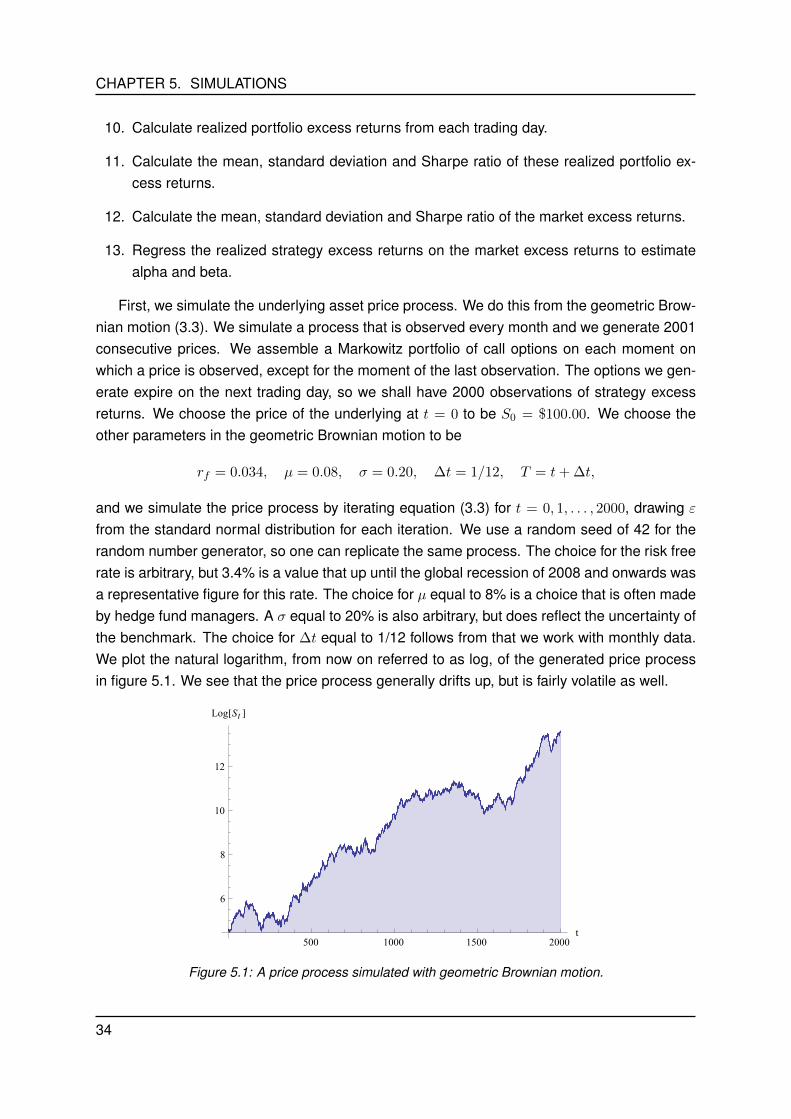
CHAPTER 5. SIMULATIONS
10. Calculate realized portfolio excess returns from each trading day.
11. Calculate the mean, standard deviation and Sharpe ratio of these realized portfolio ex-cess returns.
12. Calculate the mean, standard deviation and Sharpe ratio of the market excess returns.
13. Regress the realized strategy excess returns on the market excess returns to estimatealpha and beta.
First, we simulate the underlying asset price process. We do this from the geometric Brow-nian motion (3.3). We simulate a process that is observed every month and we generate 2001consecutive prices. We assemble a Markowitz portfolio of call options on each moment onwhich a price is observed, except for the moment of the last observation. The options we gen-erate expire on the next trading day, so we shall have 2000 observations of strategy excessreturns. We choose the price of the underlying at t = 0 to be S0 = $100.00. We choose theother parameters in the geometric Brownian motion to be
rf = 0.034, µ = 0.08, σ = 0.20, ∆t = 1/12, T = t+ ∆t,
and we simulate the price process by iterating equation (3.3) for t = 0, 1, . . . , 2000, drawing ε
from the standard normal distribution for each iteration. We use a random seed of 42 for therandom number generator, so one can replicate the same process. The choice for the risk freerate is arbitrary, but 3.4% is a value that up until the global recession of 2008 and onwards wasa representative figure for this rate. The choice for µ equal to 8% is a choice that is often madeby hedge fund managers. A σ equal to 20% is also arbitrary, but does reflect the uncertainty ofthe benchmark. The choice for ∆t equal to 1/12 follows from that we work with monthly data.We plot the natural logarithm, from now on referred to as log, of the generated price processin figure 5.1. We see that the price process generally drifts up, but is fairly volatile as well.
500 1000 1500 2000t
6
8
10
12
Log@St D
Figure 5.1: A price process simulated with geometric Brownian motion.
34
CHAPTER 5. SIMULATIONS
Throughout these simulations, we assume that the market only consists of this risky assetand a risk free rate. Therefore, we treat the underlying excess returns given by equation (3.4)as the market excess returns.
Next, we generate a range of options on the benchmark for each trading day. In the Op-tionmetrics database, there are 13 options available on each trading day and they are charac-terized by their delta, which is their sensitivity to movements in the underlying price process.In the database, the available options are options with deltas running from 0.20 through 0.80with steps of 0.05. Therefore, we adapt our simulations to this framework. On each tradingday we generate 13 options, and we start of with generating their strike prices. We solve thestrikes from the theoretical delta of European call options, which is given by the term N(d1) inthe Black-Scholes formula (3.5), which is given as
N
(1
σ√
∆t
[ln
(StKi
)+
(rf +
σ2
2
)∆t
]).
We see that the only unknown parameter in this expression is the strike Ki, hence, we cansolve the equations
N(d1) = ∆i, ∆i ∈ 0.20, 0.25, . . . , 0.80
for Ki on each trading day, giving us 13 strikes per trading day. We repeat this for every tradingday. Then, from this generated strikes, we generate the prices, Ci, for all these options withthe Black-Scholes formula (3.5). Options with a delta of 0.5 are usually interpreted in financeas at-the-money (ATM) options, hence, options for which the strike price is equal to the currentprice of the underlying. This is formally not exactly the case, but the strike is very close to thecurrent price of the underlying. A delta below 0.5 implies that the option is out-of-the-money(OTM), hence, the option has a higher strike price than the current underlying price. The lowerthe delta, the further the option is OTM. A delta above 0.5 implies that the option is in-the-money (ITM), hence, the option has a lower strike price than the current underlying price. Thehigher the delta, the further the option is ITM. We extend the range of strikes on each tradingday with a strike price of zero and the option prices with the underlying price on that trading day.
Having a price process and options available on every trading day, we compute the realizedexcess return of each option on each trading day, using equation (3.7), creating the vectorrrealizedt for t = 0, 1, . . . , 1999. The excess return of the zero strike option is equal to the excessreturn on the underlying itself. The mean, realized monthly excess return of the options in thissimulation are
0.149916, 0.130867, 0.121305, 0.115353, 0.109943, 0.104326, 0.0991952,
0.0948217, 0.0892549, 0.0823697, 0.0736303, 0.0645233, 0.0557866, 0.00335623,
where the first element is the mean, realized monthly excess return on the option with ∆ = 0.20,the second that of the option with ∆ = 0.25, continuing to the next to last element, which isthe mean, realized monthly excess return on the option with ∆ = 0.80. The last element is the
35
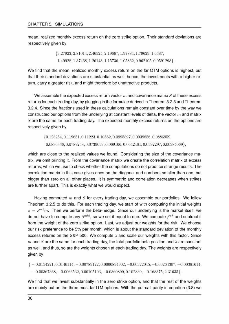
CHAPTER 5. SIMULATIONS
mean, realized monthly excess return on the zero strike option. Their standard deviations arerespectively given by
3.27923, 2.81014, 2.46525, 2.19667, 1.97884, 1.79629, 1.6387,
1.49928, 1.37468, 1.26148, 1.15736, 1.05862, 0.962105, 0.0591298.
We find that the mean, realized monthly excess return on the far OTM options is highest, butthat their standard deviations are substantial as well, hence, the investments with a higher re-turn, carry a greater risk, and might therefore be unattractive products.
We assemble the expected excess return vectorm and covariance matrix S of these excessreturns for each trading day, by plugging in the formulae derived in Theorem 3.2.3 and Theorem3.2.4. Since the fractions used in these calculations remain constant over time by the way weconstructed our options from the underlying at constant levels of delta, the vector m and matrixS are the same for each trading day. The expected monthly excess returns on the options arerespectively given by
0.128254, 0.119651, 0.11223, 0.10562, 0.0995897, 0.0939856, 0.0886959,
0.0836336, 0.0787258, 0.0739059, 0.069106, 0.0642481, 0.0592297, 0.00384069,
which are close to the realized values we found. Considering the size of the covariance ma-trix, we omit printing it. From the covariance matrix we create the correlation matrix of excessreturns, which we use to check whether the computations do not produce strange results. Thecorrelation matrix in this case gives ones on the diagonal and numbers smaller than one, butbigger than zero on all other places. It is symmetric and correlation decreases when strikesare further apart. This is exactly what we would expect.
Having computed m and S for every trading day, we assemble our portfolios. We followTheorem 3.2.5 to do this. For each trading day, we start of with computing the initial weightsπ = S−1m. Then we perform the beta-hedge. Since our underlying is the market itself, wedo not have to compute any βmkt, so we set it equal to one. We compute βpf and subtract itfrom the weight of the zero strike option. Last, we adjust our weights for the risk. We chooseour risk preference to be 5% per month, which is about the standard deviation of the monthlyexcess returns on the S&P 500. We compute λ and scale our weights with this factor. Sincem and S are the same for each trading day, the total portfolio beta position and λ are constantas well, and thus, so are the weights chosen at each trading day. The weights are respectivelygiven by
− 0.0154221, 0.0146114,−0.00789122, 0.0000894902,−0.00322045,−0.00264307,−0.00361614,
− 0.00367368,−0.0066532, 0.00105103,−0.0360899, 0.102839,−0.168375, 2.31635.
We find that we invest substantially in the zero strike option, and that the rest of the weightsare mainly put on the three most far ITM options. With the put-call parity in equation (3.8) we
36
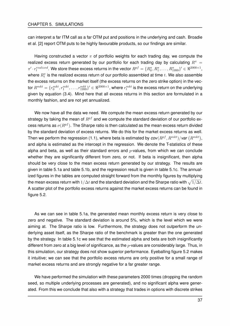
CHAPTER 5. SIMULATIONS
can interpret a far ITM call as a far OTM put and positions in the underlying and cash. Broadieet al. [2] report OTM puts to be highly favourable products, so our findings are similar.
Having constructed a vector π of portfolio weights for each trading day, we compute therealized excess return generated by our portfolio for each trading day by calculating Rπ =
π′ · rrealizedt . We store these excess returns in the vector Rpf = Rπ0 , Rπ1 , . . . , Rπ1999′ ∈ <2000×1,where Rπt is the realized excess return of our portfolio assembled at time t. We also assemblethe excess returns on the market itself (the excess returns on the zero strike option) in the vec-tor Rmkt = rmkt0 , rmkt1 , . . . , rmkt1999′ ∈ <2000×1, where rmktt is the excess return on the underlyinggiven by equation (3.4). Mind here that all excess returns in this section are formulated in amonthly fashion, and are not yet annualized.
We now have all the data we need. We compute the mean excess return generated by ourstrategy by taking the mean of Rpf and we compute the standard deviation of our portfolio ex-cess returns as σ(Rpf ). The Sharpe ratio is then calculated as the mean excess return dividedby the standard deviation of excess returns. We do this for the market excess returns as well.Then we perform the regression (1.1), where beta is estimated by cov(Rpf , Rmkt)/var
(Rmkt
),
and alpha is estimated as the intercept in the regression. We denote the T-statistics of thesealpha and beta, as well as their standard errors and p-values, from which we can concludewhether they are significantly different from zero, or not. If beta is insignificant, then alphashould be very close to the mean excess return generated by our strategy. The results aregiven in table 5.1a and table 5.1b, and the regression result is given in table 5.1c. The annual-ized figures in the tables are computed straight forward from the monthly figures by multiplyingthe mean excess return with 1/∆t and the standard deviation and the Sharpe ratio with
√1/∆t.
A scatter plot of the portfolio excess returns against the market excess returns can be found infigure 5.2.
As we can see in table 5.1a, the generated mean monthly excess return is very close tozero and negative. The standard deviation is around 5%, which is the level which we wereaiming at. The Sharpe ratio is low. Furthermore, the strategy does not outperform the un-derlying asset itself, as the Sharpe ratio of the benchmark is greater than the one generatedby the strategy. In table 5.1c we see that the estimated alpha and beta are both insignificantlydifferent from zero at a big level of significance, as the p-values are considerably large. Thus, inthis simulation, our strategy does not show superior performance. Eyeballing figure 5.2 makesit intuitive; we can see that the portfolio excess returns are only positive for a small range ofmarket excess returns and are strongly negative for a far greater range.
We have performed the simulation with these parameters 2000 times (dropping the randomseed, so multiple underlying processes are generated), and no significant alpha were gener-ated. From this we conclude that also with a strategy that trades in options with discrete strikes
37
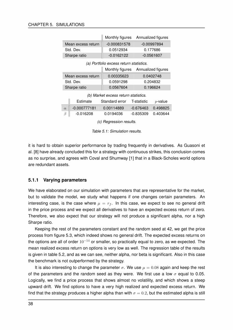
CHAPTER 5. SIMULATIONS
Monthly figures Annualized figures
Mean excess return -0.000831578 -0.00997894Std. Dev. 0.0512934 0.177686Sharpe ratio -0.0162122 -0.0561607
(a) Portfolio excess return statistics.Monthly figures Annualized figures
Mean excess return 0.00335623 0.0402748Std. Dev. 0.0591298 0.204832Sharpe ratio 0.0567604 0.196624
(b) Market excess return statistics.Estimate Standard error T-statistic p-value
α -0.000777181 0.00114889 -0.676463 0.498825β -0.016208 0.0194036 -0.835309 0.403644
(c) Regression results.
Table 5.1: Simulation results.
it is hard to obtain superior performance by trading frequently in derivatives. As Guasoni etal. [8] have already concluded this for a strategy with continuous strikes, this conclusion comesas no surprise, and agrees with Coval and Shumway [1] that in a Black-Scholes world optionsare redundant assets.
5.1.1 Varying parameters
We have elaborated on our simulation with parameters that are representative for the market,but to validate the model, we study what happens if one changes certain parameters. Aninteresting case, is the case where µ = rf . In this case, we expect to see no general driftin the price process and we expect all derivatives to have an expected excess return of zero.Therefore, we also expect that our strategy will not produce a significant alpha, nor a highSharpe ratio.
Keeping the rest of the parameters constant and the random seed at 42, we get the priceprocess from figure 5.3, which indeed shows no general drift. The expected excess returns onthe options are all of order 10−14 or smaller, so practically equal to zero, as we expected. Themean realized excess return on options is very low as well. The regression table of the resultsis given in table 5.2, and as we can see, neither alpha, nor beta is significant. Also in this casethe benchmark is not outperformed by the strategy.
It is also interesting to change the parameter σ. We use µ = 0.08 again and keep the restof the parameters and the random seed as they were. We first use a low σ equal to 0.05.Logically, we find a price process that shows almost no volatility, and which shows a steepupward drift. We find options to have a very high realized and expected excess return. Wefind that the strategy produces a higher alpha than with σ = 0.2, but the estimated alpha is still
38
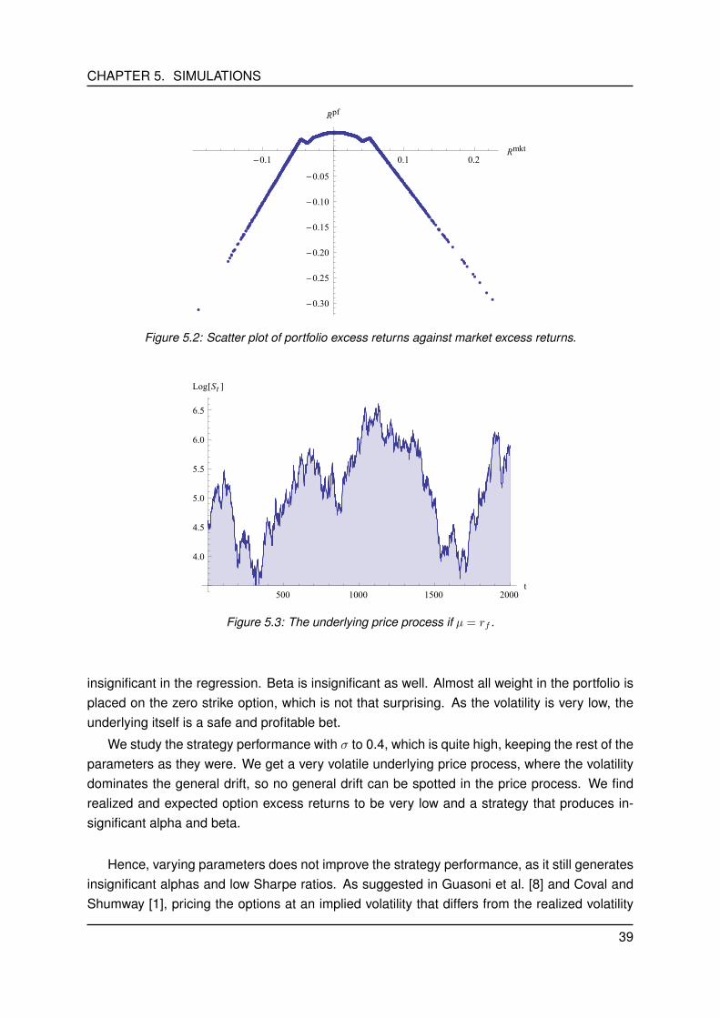
CHAPTER 5. SIMULATIONS
-0.1 0.1 0.2Rmkt
-0.30
-0.25
-0.20
-0.15
-0.10
-0.05
Rpf
Figure 5.2: Scatter plot of portfolio excess returns against market excess returns.
500 1000 1500 2000t
4.0
4.5
5.0
5.5
6.0
6.5
Log@St D
Figure 5.3: The underlying price process if µ = rf .
insignificant in the regression. Beta is insignificant as well. Almost all weight in the portfolio isplaced on the zero strike option, which is not that surprising. As the volatility is very low, theunderlying itself is a safe and profitable bet.
We study the strategy performance with σ to 0.4, which is quite high, keeping the rest of theparameters as they were. We get a very volatile underlying price process, where the volatilitydominates the general drift, so no general drift can be spotted in the price process. We findrealized and expected option excess returns to be very low and a strategy that produces in-significant alpha and beta.
Hence, varying parameters does not improve the strategy performance, as it still generatesinsignificant alphas and low Sharpe ratios. As suggested in Guasoni et al. [8] and Coval andShumway [1], pricing the options at an implied volatility that differs from the realized volatility
39

CHAPTER 5. SIMULATIONS
Estimate Standard error T-statistic p-value
α -0.000529743 0.0011316 -0.468135 0.639739β -0.00586368 0.0192153 -0.305157 0.760278
Table 5.2: Regression results for the case µ = rf .
on the underlying produces significant excess returns on options. In the chapter 6 we studythe strategy performance in this setting, where we use actual market data, so the option pricesdeviate from the ones given by the Black-Scholes formula used with the volatility of the under-lying.
5.2 Simulations with multiple benchmark assets
In this section we study the performance of the investment strategy derived in chapter 4 withsimulated data. We study the strategy that dynamically invests in options on two benchmarkassets. Again, we explain our simulation step by step and thereafter we elaborate on theresults. The steps that we take are as follows:
1. Generate two, underlying price processes from geometric Brownian motions with certainparameters, which are correlated in the Brownian motion terms. Consider the excessreturns on the first benchmark as the excess returns on the market.
2. For each trading day, generate a range of strikes (including the zero strike) of Europeancall options on both of the benchmark assets.
3. Use the Black-Scholes formula to calculate the call option prices corresponding to thesestrikes for each trading day. Use the benchmark prices as the prices of the zero strikeoptions on each trading day.
4. Calculate the realized excess returns on all available derivatives on both underlying oneach trading day. The excess return on the zero strike option on the first benchmark isthe excess return on the market.
5. Calculate the expected excess returns on all available derivatives on both underlying andassemble the vector m on each trading day.
6. Calculate the covariance matrix of excess returns S for each trading day.
7. Calculate initial weights for each trading day.
8. Perform a beta-hedge on the weights of both underlying on each day.
9. Adjust the weights for a certain level of risk on each trading day.
10. Calculate realized portfolio excess returns from each trading day.
40
CHAPTER 5. SIMULATIONS
11. Calculate the mean, standard deviation and Sharpe ratio of these realized portfolio ex-cess returns.
12. Calculate the mean, standard deviation and Sharpe ratio of excess returns on both un-derlying.
13. Regress the realized strategy excess returns on the market excess returns to estimatealpha and beta.
We start with simulating the underlying price processes. We generate them both with ageometric Brownian motion, each with its own parameters, but we need to generate themin such a way that the geometric Brownian motions are correlated in the Brownian motionterms. We simulate processes that are observed monthly and we generate 2001 consecutiveprices. We assemble a Markowitz portfolio of call options on each moment on which a priceis observed, except for the moment of the last observation. The options we generate expireon the next trading day, so we shall have 2000 observations of strategy excess returns. Wechoose the price of the underlying at t = 0 to be S(1)
0 = $100 and S(2)0 = $420. The parameters
we use are as follows:
rf = 0.034, µ1 = 0.07, µ2 = 0.08, σ1 = 0.20, σ2 = 0.22, ρ12 = 0.9, ∆t = 1/12.
and we simulate the price processes by iterating equation (3.3) for t = 0, 1, . . . , 2000 for bothunderlying, but to make them correlated, we do not simply draw ε1 and ε2 separately from thestandard normal distribution. We first construct 2 strings of 2001 standard normal distributeddrawings, x1 and x2. Then we define η1 = x2 and η2 = ρ12x1 + x2
√1− ρ2
12, which are now twostrings with correlation ρ12. Now, in stead of drawing ε1 and ε2 for each trading day, we use thenext element in η1 and η2 respectively. The choice of parameters is again to match reality andare all but ρ12 explained by the same reasoning as in section 5.1 . We choose the correlationto be fairly high, because the indices which we work with in the market data analysis in chapter6 exhibit a large correlation as well. We plot the log of the resulting price processes in figure5.4, in which we see that the price processes show similar movements due to the correlationin their Brownian motion terms.
Next, we generate a range of options on both underlying on every trading day. We do this inthe same way as in the one dimensional simulation for both underlying, but with less availablestrikes on both. As we have seen in the one dimensional case, most of the weight was put onfar ITM options, and if we would use 14 options on both assets, the covariance matrix wouldbecome quite big, so we choose to use only the range of ATM to ITM options (deltas runningfrom 0.50 to 0.80 in steps op 0.05) on both underlying. We again use the Black-Scholes for-mula (3.5) to compute all option prices and we extend both ranges of strikes with a zero strikeon each trading day, and add their prices to our option prices (which are equal to S(1)
t and S(2)t
on trading day t respectively), resulting in 8 available European call options per underlying pertrading day.
41
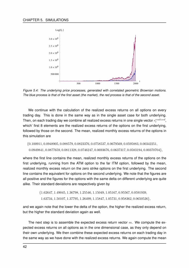
CHAPTER 5. SIMULATIONS
500 1000 1500 2000t
500000
1.0 ´ 106
1.5 ´ 106
2.0 ´ 106
2.5 ´ 106
3.0 ´ 106
Log@St D
Figure 5.4: The underlying price processes, generated with correlated geometric Brownian motions.The blue process is that of the first asset (the market), the red process is that of the second asset.
We continue with the calculation of the realized excess returns on all options on everytrading day. This is done in the same way as in the single asset case for both underlying.Then, on each trading day we combine all realized excess returns in one single vector rrealizedt ,which’ first 8 elements are the realized excess returns of the options on the first underlying,followed by those on the second. The mean, realized monthly excess returns of the options inthis simulation are
0.100911, 0.0948905, 0.088579, 0.0823376, 0.0758537, 0.0679569, 0.0595883, 0.00342251,
0.0949841, 0.0877659, 0.0811328, 0.0746247, 0.0693676, 0.0637317, 0.0583194, 0.00370704,
where the first line contains the mean, realized monthly excess returns of the options on thefirst underlying, running from the ATM option to the far ITM option, followed by the mean,realized monthly excess return on the zero strike options on the first underlying. The secondline contains the equivalent for options on the second underlying. We note that the figures areall positive and the figures for the options with the same delta on different underlying are quitealike. Their standard deviations are respectively given by
1.62647, 1.49045, 1.36798, 1.25546, 1.15049, 1.05167, 0.95567, 0.0591939,
1.63734, 1.50107, 1.37795, 1.26499, 1.15847, 1.05731, 0.958362, 0.0650526,
and we again note that the lower the delta of the option, the higher the realized excess return,but the higher the standard deviation again as well.
The next step is to assemble the expected excess return vector m. We compute the ex-pected excess returns on all options as in the one dimensional case, as they only depend ontheir own underlying. We then combine these expected excess returns on each trading day inthe same way as we have done with the realized excess returns. We again compute the mean
42
CHAPTER 5. SIMULATIONS
expected excess returns:
0.0689959, 0.0650948, 0.0613083, 0.0575854, 0.0538736, 0.0501125, 0.0462224, 0.0030045,
0.0807276, 0.0761497, 0.0717092, 0.0673457, 0.062998, 0.0585954, 0.0540445, 0.00384069,
which are again close to the realized values.
We assemble the covariance matrix S on each trading day. Considering the representationfor S given in equation (4.1), on each trading day we first calculate S11 and S22 as in the singleasset case. Then, we calculate S12 in a few steps. We first calculate the covariances of type1 with equation (4.3). Then we calculate the covariances of type 2 and 3 with the rest of theequations provided by Theorem 4.1.1. We combine the calculated terms to one matrix, and wetranspose this matrix to get S21. Then we combine all these matrices to one covariance matrixS, and from this covariance matrix, we can generate the correlation matrix. Again, all fractionsused in the explicit formulae to calculate m and S are constant over time, so m and S areconstant over time. Considering the sizes of the covariance and correlation matrices, we omitprinting them. The correlation matrix does show the behaviour that we would expect; the cor-relations in the S12 and S21 parts of the correlation matrix decrease as strikes drift further apart.
Having computed m and S for every trading day, we again assemble our portfolios. Forthis, we use Theorem 4.1.2 on each trading day. The initial weights are computed, and then thebeta-hedge is performed. We compute the beta with respect to the first underlying and subtractthis weight from its zero strike option. Then we calculate the beta position with respect to thesecond underlying with these adjusted weights, and subtract this position from the weight ofthe zero strike option on the second underlying. Hence, we assume that the βmkt2 is equal toone, which is not a bad assumption, as the correlation between the assets is very high. Thenwe adjust for 5% risk per month again, by calculating λ and adjusting the weights with thisfactor. Since m and S are constant over time, the weights will be constant as well. In the sameorder that we have used for the other vectors we presented, we find them to be
− 0.00400262, 0.00656925,−0.00157441, 0.00120184,−0.000811391, 0.00481288,−0.00363784,−2.00319,
− 0.0227464, 0.024274,−0.00917854, 0.00216984,−0.00789276, 0.0191966,−0.0324392, 2.03059.
For both assets we see that most weight is on the zero strike option again, and we cannotconclude that a certain kind of option is favourable along with the zero strike option, as all ofthe other weights are quite alike.
Having our vector π of portfolio weights on each trading day, we can again compute therealized excess returns generated by our portfolios by calculating Rπ = π′ · rrealizedt . We storethese excess returns in a vector Rpf again, like in the one dimensional case, and we assemblethe excess returns on the market itself (the excess returns on the zero strike option of the firstunderlying) in the vector Rmkt, as in the one dimensional case. Note that these excess returns
43
CHAPTER 5. SIMULATIONS
throughout this section are all formulated in a monthly fashion, and are not yet annualized.
We proceed as in the one dimensional case by calculating the mean of Rpf and its standarddeviation. Then we compute the Sharpe ratio. We do this for both benchmark assets as well.All figures can be annualized in the same way as we described in the one dimensional case.Then, we regress the strategy excess returns on the market excess returns to estimate alphaand beta, and we denote the standard error of the estimates, their T-statistics and their p-values. We report the results in table 5.3.
Monthly figures Annualized figures
Mean excess return -0.000929554 -0.0111546Std. Dev. 0.050492 0.17491Sharpe ratio -0.0184099 -0.0637738
(a) Portfolio excess return statistics.Monthly figures Annualized figures
Mean excess return 0.00342251 0.0410701Std. Dev. 0.0591939 0.205054Sharpe ratio 0.0578186 0.200289
(b) Market excess return statistics.Monthly figures Annualized figures
Mean excess return 0.00370704 0.0444845Std. Dev. 0.0650526 0.225349Sharpe ratio 0.0569853 0.197403
(c) Second underlying excess return statistics.Estimate Standard error T-statistic p-value
α 0.000321253 0.00102212 0.314301 0.753325β -0.365465 0.0172428 -21.1952 0
(d) Regression results.
Table 5.3: Simulation results.
As we can see in table 5.3a, the generated mean monthly excess return is very close tozero and negative. The standard deviation of strategy excess returns is around 5%, the levelwe were aiming at, and the Sharpe ratio is small. The strategy does not outperform eitherof the benchmarks, which generate higher Sharpe ratios, as can be found in tables 5.3b and5.3c. In table 5.3d we see that the estimated alpha is insignificantly different from zero at abig level of significance. However, the beta is significant, which shows that the beta-hedgefailed in this case. This is probably due to overcompensation in the hedging; we subtract thebeta position with respect to the market from the weight on the zero strike option of the firstunderlying, making the market beta position of the portfolio equal to zero. Since the correlationbetween the underlying is high, this would almost imply that the beta position with respect tothe second underlying is zero as well, but we still compensate for it. Therefore, there might
44
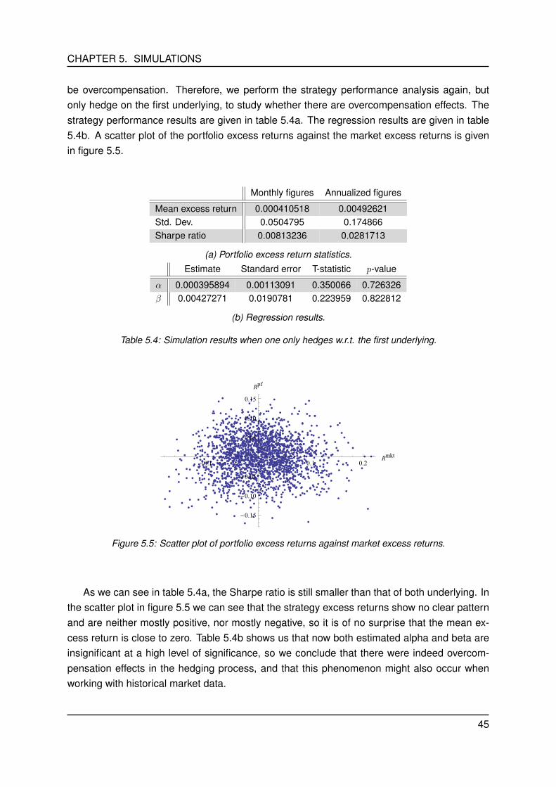
CHAPTER 5. SIMULATIONS
be overcompensation. Therefore, we perform the strategy performance analysis again, butonly hedge on the first underlying, to study whether there are overcompensation effects. Thestrategy performance results are given in table 5.4a. The regression results are given in table5.4b. A scatter plot of the portfolio excess returns against the market excess returns is givenin figure 5.5.
Monthly figures Annualized figures
Mean excess return 0.000410518 0.00492621Std. Dev. 0.0504795 0.174866Sharpe ratio 0.00813236 0.0281713
(a) Portfolio excess return statistics.Estimate Standard error T-statistic p-value
α 0.000395894 0.00113091 0.350066 0.726326β 0.00427271 0.0190781 0.223959 0.822812
(b) Regression results.
Table 5.4: Simulation results when one only hedges w.r.t. the first underlying.
-0.1 0.1 0.2Rmkt
-0.15
-0.10
-0.05
0.05
0.10
0.15
Rpf
Figure 5.5: Scatter plot of portfolio excess returns against market excess returns.
As we can see in table 5.4a, the Sharpe ratio is still smaller than that of both underlying. Inthe scatter plot in figure 5.5 we can see that the strategy excess returns show no clear patternand are neither mostly positive, nor mostly negative, so it is of no surprise that the mean ex-cess return is close to zero. Table 5.4b shows us that now both estimated alpha and beta areinsignificant at a high level of significance, so we conclude that there were indeed overcom-pensation effects in the hedging process, and that this phenomenon might also occur whenworking with historical market data.
45
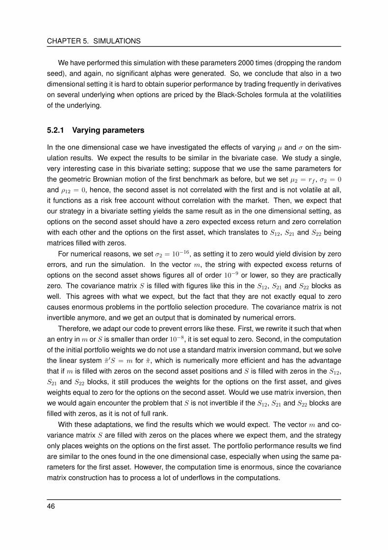
CHAPTER 5. SIMULATIONS
We have performed this simulation with these parameters 2000 times (dropping the randomseed), and again, no significant alphas were generated. So, we conclude that also in a twodimensional setting it is hard to obtain superior performance by trading frequently in derivativeson several underlying when options are priced by the Black-Scholes formula at the volatilitiesof the underlying.
5.2.1 Varying parameters
In the one dimensional case we have investigated the effects of varying µ and σ on the sim-ulation results. We expect the results to be similar in the bivariate case. We study a single,very interesting case in this bivariate setting; suppose that we use the same parameters forthe geometric Brownian motion of the first benchmark as before, but we set µ2 = rf , σ2 = 0
and ρ12 = 0, hence, the second asset is not correlated with the first and is not volatile at all,it functions as a risk free account without correlation with the market. Then, we expect thatour strategy in a bivariate setting yields the same result as in the one dimensional setting, asoptions on the second asset should have a zero expected excess return and zero correlationwith each other and the options on the first asset, which translates to S12, S21 and S22 beingmatrices filled with zeros.
For numerical reasons, we set σ2 = 10−16, as setting it to zero would yield division by zeroerrors, and run the simulation. In the vector m, the string with expected excess returns ofoptions on the second asset shows figures all of order 10−9 or lower, so they are practicallyzero. The covariance matrix S is filled with figures like this in the S12, S21 and S22 blocks aswell. This agrees with what we expect, but the fact that they are not exactly equal to zerocauses enormous problems in the portfolio selection procedure. The covariance matrix is notinvertible anymore, and we get an output that is dominated by numerical errors.
Therefore, we adapt our code to prevent errors like these. First, we rewrite it such that whenan entry in m or S is smaller than order 10−8, it is set equal to zero. Second, in the computationof the initial portfolio weights we do not use a standard matrix inversion command, but we solvethe linear system π′S = m for π, which is numerically more efficient and has the advantagethat if m is filled with zeros on the second asset positions and S is filled with zeros in the S12,S21 and S22 blocks, it still produces the weights for the options on the first asset, and givesweights equal to zero for the options on the second asset. Would we use matrix inversion, thenwe would again encounter the problem that S is not invertible if the S12, S21 and S22 blocks arefilled with zeros, as it is not of full rank.
With these adaptations, we find the results which we would expect. The vector m and co-variance matrix S are filled with zeros on the places where we expect them, and the strategyonly places weights on the options on the first asset. The portfolio performance results we findare similar to the ones found in the one dimensional case, especially when using the same pa-rameters for the first asset. However, the computation time is enormous, since the covariancematrix construction has to process a lot of underflows in the computations.
46

CHAPTER 5. SIMULATIONS
We conclude that when very small numerical errors are encountered, the strategy canproduce very erroneous results, hence, we use the alterations made to the code to solve thesenumerical errors in our market data analysis as well.
47


CHAPTER 6
MARKET DATA AND STRATEGY
PERFORMANCE ANALYSIS
In this chapter we study the performance of the strategies derived in chapters 3 and 4 withhistorical market data. We test the strategies in a one dimensional setting and in a two dimen-sional setting. We use market data from the Optionmetrics database, running from January 4th1996 to January 31st 2013. We consider the S&P 500, the NASDAQ 100, the Russell 2000and the Dow Jones 1/100th Industrial Average in our analyses. Throughout our entire dataanalysis, we will consider the S&P 500 as “the market”. The database contains all historicalprices on these assets, the realized volatility of these assets and an annualized risk free rateon every date. Although the database contains data on all historical traded options on theseassets, we use another table of the database for the option data; the volatility surface table.This table contains the interpolated volatility surface for each asset on each day, establishedusing a methodology based on a kernel smoothing algorithm and the actual traded options.This table contains information on standardized options on every business day with a range offixed expirations. The options are available at a range of deltas of 0.20 to 0.80 with steps of0.05.
In the first section of this chapter we provide a visualization and analysis of the data onthe underlying assets. In the second section we explain our analysis methodology used inthe single asset case and we then perform our strategy performance analysis over differentperiods of time and with settings, and then present the results. The same is done for the twodimensional case in the third section.
6.1 Historical data on the benchmark assets
In this section we provide a visualization and an analysis of the underlying price processes weconsider in our analyses, of their realized volatilities and of the risk free rate over time.
The S&P 500 index consists of 500 leading companies publicly traded in the US stock mar-ket. Therefore it is a suitable candidate to represent “the market”, thus, throughout this wholechapter we use the excess returns on the S&P 500 as the market excess returns. The NAS-DAQ 100 consists of the 100 largest non-financial companies listed on the NASDAQ, whichcontains a lot of stocks in technological companies. The Russell 2000 is a small capitalization
49

CHAPTER 6. MARKET DATA AND STRATEGY PERFORMANCE ANALYSIS
stock market index of the bottom 2000 stocks in the Russell 3000 index, and the Dow Jones1/100th Average Industrial index is the Dow Jones Industrial Average, an index that shows theperformance of 30 large publicly owned companies in the US, scaled by 1/100.
In figure 6.1 we present the underlying price processes of the four underlying assets. Weobserve the close of each underlying asset on every first trading day of the month, over theentire period of available data. We use these closing prices as the underlying prices in ouranalyses. We see that the S&P 500 and NASDAQ 100 have data available starting fromJanuary 1996, the Russell 2000 from January 1997 and the first available data of the DowJones 1/100th is from January 1998. For all indices we have data available until January31st 2013. In figure 6.1 we clearly see the effects of the Dot-com bubble for all assets. This
2000 2005 2010600
800
1000
1200
1400
(a) S&P 500.
2000 2005 2010500
1000
1500
2000
2500
3000
3500
4000
(b) NASDAQ 100.
2000 2005 2010
400
500
600
700
800
900
(c) Russell 2000.
2000 2005 2010
70
80
90
100
110
120
130
140
(d) Dow Jones 1/100th.
Figure 6.1: Historical underlying price processes, prices are given in US dollars.
Internet bubble was a historic speculative bubble during the period of 1997-2000, and burstin March 2000. The effects for the S&P 500 and NASDAQ 100 are most clear; the pricesrise steeply in the period 1997-2000, even reaching 4000 for the NASDAQ 100, and then theymake an enormous drop after March 2000. The magnitude of the effects on the NASDAQ 100is explained by the fact that the NASDAQ 100 contains a lot of technological stocks, whichwere of course most affected by a bubble in the Internet section. We also see the effects ofthe recent credit crisis on all assets; after the burst of the Dot-com bubble we see prices risingagain in early 2003. The prices continue to rise, until 2007, when the credit crisis kicked in,
50
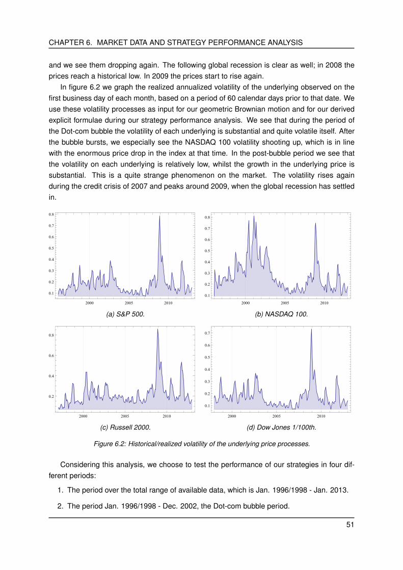
CHAPTER 6. MARKET DATA AND STRATEGY PERFORMANCE ANALYSIS
and we see them dropping again. The following global recession is clear as well; in 2008 theprices reach a historical low. In 2009 the prices start to rise again.
In figure 6.2 we graph the realized annualized volatility of the underlying observed on thefirst business day of each month, based on a period of 60 calendar days prior to that date. Weuse these volatility processes as input for our geometric Brownian motion and for our derivedexplicit formulae during our strategy performance analysis. We see that during the period ofthe Dot-com bubble the volatility of each underlying is substantial and quite volatile itself. Afterthe bubble bursts, we especially see the NASDAQ 100 volatility shooting up, which is in linewith the enormous price drop in the index at that time. In the post-bubble period we see thatthe volatility on each underlying is relatively low, whilst the growth in the underlying price issubstantial. This is a quite strange phenomenon on the market. The volatility rises againduring the credit crisis of 2007 and peaks around 2009, when the global recession has settledin.
2000 2005 2010
0.1
0.2
0.3
0.4
0.5
0.6
0.7
0.8
(a) S&P 500.
2000 2005 2010
0.1
0.2
0.3
0.4
0.5
0.6
0.7
0.8
(b) NASDAQ 100.
2000 2005 2010
0.2
0.4
0.6
0.8
(c) Russell 2000.
2000 2005 2010
0.1
0.2
0.3
0.4
0.5
0.6
0.7
(d) Dow Jones 1/100th.
Figure 6.2: Historical/realized volatility of the underlying price processes.
Considering this analysis, we choose to test the performance of our strategies in four dif-ferent periods:
1. The period over the total range of available data, which is Jan. 1996/1998 - Jan. 2013.
2. The period Jan. 1996/1998 - Dec. 2002, the Dot-com bubble period.
51
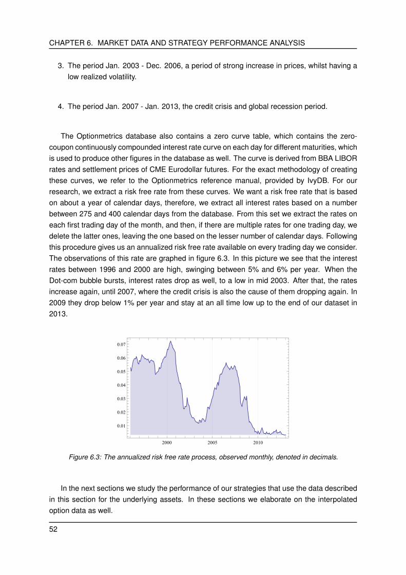
CHAPTER 6. MARKET DATA AND STRATEGY PERFORMANCE ANALYSIS
3. The period Jan. 2003 - Dec. 2006, a period of strong increase in prices, whilst having alow realized volatility.
4. The period Jan. 2007 - Jan. 2013, the credit crisis and global recession period.
The Optionmetrics database also contains a zero curve table, which contains the zero-coupon continuously compounded interest rate curve on each day for different maturities, whichis used to produce other figures in the database as well. The curve is derived from BBA LIBORrates and settlement prices of CME Eurodollar futures. For the exact methodology of creatingthese curves, we refer to the Optionmetrics reference manual, provided by IvyDB. For ourresearch, we extract a risk free rate from these curves. We want a risk free rate that is basedon about a year of calendar days, therefore, we extract all interest rates based on a numberbetween 275 and 400 calendar days from the database. From this set we extract the rates oneach first trading day of the month, and then, if there are multiple rates for one trading day, wedelete the latter ones, leaving the one based on the lesser number of calendar days. Followingthis procedure gives us an annualized risk free rate available on every trading day we consider.The observations of this rate are graphed in figure 6.3. In this picture we see that the interestrates between 1996 and 2000 are high, swinging between 5% and 6% per year. When theDot-com bubble bursts, interest rates drop as well, to a low in mid 2003. After that, the ratesincrease again, until 2007, where the credit crisis is also the cause of them dropping again. In2009 they drop below 1% per year and stay at an all time low up to the end of our dataset in2013.
2000 2005 2010
0.01
0.02
0.03
0.04
0.05
0.06
0.07
Figure 6.3: The annualized risk free rate process, observed monthly, denoted in decimals.
In the next sections we study the performance of our strategies that use the data describedin this section for the underlying assets. In these sections we elaborate on the interpolatedoption data as well.
52

CHAPTER 6. MARKET DATA AND STRATEGY PERFORMANCE ANALYSIS
6.2 Strategy performance analysis with a single benchmark asset
In this section we study the performance of our derived strategy for the one dimensional casewith historical market data. We first elaborate on how our analysis is performed and then testour one dimensional strategy on all four underlying assets, over all four periods mentioned inthe previous section. We study the effect of the three options we have for the choice of βmkt
in Theorem 3.2.5. Then we implement the model extensions as proposed in section 3.3 andtest them with the S&P 500. We shall also perform a regression on our strategy excess returnswith the market returns and the other Fama & French factors as explanatory variables; themarket capitalization factor (SMB) and the book-to-market factor (HML), which are available atKenneth French’s website. The tables on individual option analysis can be found in AppendixB.
6.2.1 Methodology
We trade on every first business day of the month, which thus will be our trading days. Weassume that the underlying price process follows a geometric Brownian motion with µ = 0.08
and σ equal to the realized volatility of the underlying at the current trading day. On everytrading day, we have a range of 13 standardized European call options available from theOptionmetrics database, which all expire in 30 calendar days, thus, we will use a ∆t of 1/12.The deltas of the options run from 0.20 to 0.80 in steps of 0.05 and the corresponding strikeprices and option prices are provided in the Optionmetrics database. For each trading day weadd the zero strike option with a price equal to the underlying price on the that trading day andan expiration of 30 calendar days to this set of options. Since expiration in 30 calendar daysdoes not necessarily have to correspond to our next trading day, we construct a vector whichcontains the underlying price at expiration of the options, or, if they expire on a non-businessday, the price on the closest preceding business day. This is thus the vector containing allvalues for ST .
Given these values of ST we calculate the realized excess return on all options and on theunderlying itself in the same way as in section 5.1, but using the market dictated values for allvariables.
We proceed with the calculation of the expected excess returns on all options on all tradingdays, the assembly of m on each trading day, and then with the calculation of the elements ofthe covariance matrix S and its assembly on each trading day. To avoid numerical errors dueto plugging in zeros for these calculations with the zero strike option, we use equations (3.12)and (3.15) to calculate mn and cov(roptn , roptn ) on each trading day, where n indicates the zerostrike option.
Then we calculate our portfolio weights on each trading day, in the same way as in section5.1, but with the option of choosing βmkt unequal to one, for which we explain the methodologyat the end of this section. Then, we compute the excess return generated by our portfoliochoice on each trading day and collect them in a vector Rpf . We compute the mean excess
53

CHAPTER 6. MARKET DATA AND STRATEGY PERFORMANCE ANALYSIS
return, the standard deviation of the excess returns and the Sharpe ratio of our strategy, whichis the fraction of these respective figures.
We then regress the strategy excess returns on the market excess returns. The marketexcess returns are in this case the realized excess returns on the S&P 500 during the tradingperiods, so we need to compute them once for every trading day and import them in the analy-ses on the other indices. We use the excess returns on the zero strike options on the S&P 500for this cause. The regression gives us the estimates of alpha and beta, the standard errorsof these estimates, their T-statistics and their p-values. From these statistics we can concludewhether the estimates of alpha and beta are statistically different from zero or not at a certainlevel of significance. We always use a 5% significance level, unless we mention otherwise.We also regress the realized portfolio excess returns on the market excess returns and on theother Fama & French factors, SMB and HML, and study whether the betas belonging to thesefactors are significant or not.
The remaining question is how to calculate βmkt when one deviates from the assumptionsthat it is equal to one. We have two options; use a period prior to our first trading day tocalculate it and then keep it constant throughout the entire period of analysis, or updating itdynamically by computing it each trading day, using a period prior to our first trading day tocompute the βmkt on our first trading day and then updating it on every new trading day, byadding the observed underlying and market excess returns from the previous trading day to thevectors of excess returns generated in the period before our first trade, used in the calculationof βmkt.
The first option is straightforward. We choose the length of the period prior to our first tradeand we compute the monthly excess returns on our underlying asset and on the S&P 500during this period. We then take the covariance of these excess returns divided by the varianceof the excess returns on the S&P 500, which gives us βmkt. If we analyze our strategy runningfrom 1996, then we can import the underlying data from Yahoo! Finance for the period. If weuse periods that start later, we can use Optionmetrics data as well.
The second option is quite like the first, but we compute βmkt on every trading day. Westart by doing the same as with the fixed beta method; we use a period prior to our first tradeto calculate excess returns on the underlying and the market and we then compute βmkt fromthis data, which we use as βmkt on our first trading day. Then, every next trading day weadd the observed excess returns on the underlying and the market to our vectors used in thecalculation of βmkt and compute it again. In this way, the market beta of the underlying isadapted to events on the market.
6.2.2 Results
In this subsection we present the results generated with our one dimensional strategy. We an-alyze the strategy performance on our four indices during the four periods mentioned in section6.1. We then analyze the effect of the different choices for βmkt and we then test our model
54
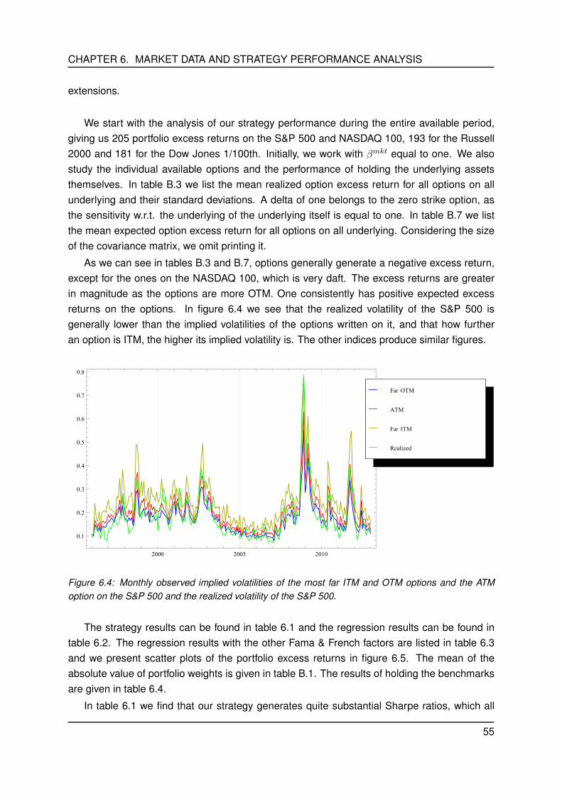
CHAPTER 6. MARKET DATA AND STRATEGY PERFORMANCE ANALYSIS
extensions.
We start with the analysis of our strategy performance during the entire available period,giving us 205 portfolio excess returns on the S&P 500 and NASDAQ 100, 193 for the Russell2000 and 181 for the Dow Jones 1/100th. Initially, we work with βmkt equal to one. We alsostudy the individual available options and the performance of holding the underlying assetsthemselves. In table B.3 we list the mean realized option excess return for all options on allunderlying and their standard deviations. A delta of one belongs to the zero strike option, asthe sensitivity w.r.t. the underlying of the underlying itself is equal to one. In table B.7 we listthe mean expected option excess return for all options on all underlying. Considering the sizeof the covariance matrix, we omit printing it.
As we can see in tables B.3 and B.7, options generally generate a negative excess return,except for the ones on the NASDAQ 100, which is very daft. The excess returns are greaterin magnitude as the options are more OTM. One consistently has positive expected excessreturns on the options. In figure 6.4 we see that the realized volatility of the S&P 500 isgenerally lower than the implied volatilities of the options written on it, and that how furtheran option is ITM, the higher its implied volatility is. The other indices produce similar figures.
2000 2005 2010
0.1
0.2
0.3
0.4
0.5
0.6
0.7
0.8
Realized
Far ITM
ATM
Far OTM
Figure 6.4: Monthly observed implied volatilities of the most far ITM and OTM options and the ATMoption on the S&P 500 and the realized volatility of the S&P 500.
The strategy results can be found in table 6.1 and the regression results can be found intable 6.2. The regression results with the other Fama & French factors are listed in table 6.3and we present scatter plots of the portfolio excess returns in figure 6.5. The mean of theabsolute value of portfolio weights is given in table B.1. The results of holding the benchmarksare given in table 6.4.
In table 6.1 we find that our strategy generates quite substantial Sharpe ratios, which all
55
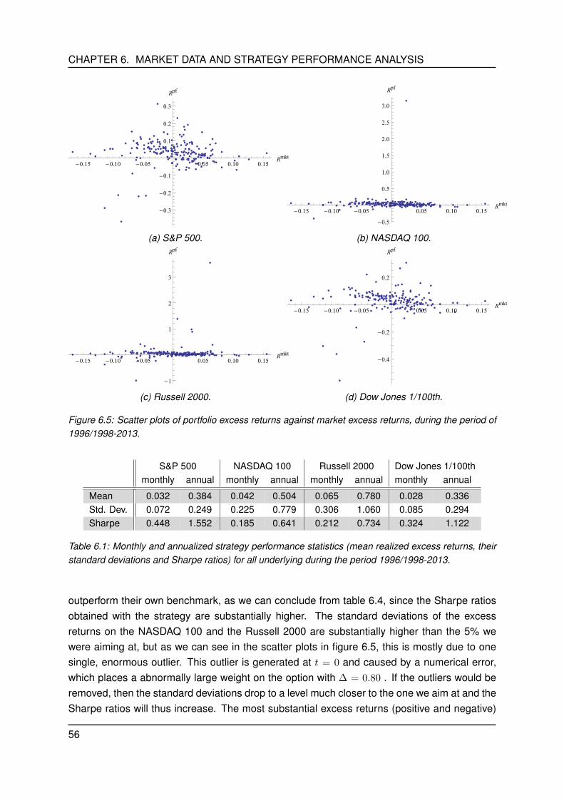
CHAPTER 6. MARKET DATA AND STRATEGY PERFORMANCE ANALYSIS
-0.15 -0.10 -0.05 0.05 0.10 0.15Rmkt
-0.3
-0.2
-0.1
0.1
0.2
0.3
Rpf
(a) S&P 500.
-0.15 -0.10 -0.05 0.05 0.10 0.15Rmkt
-0.5
0.5
1.0
1.5
2.0
2.5
3.0
Rpf
(b) NASDAQ 100.
-0.15 -0.10 -0.05 0.05 0.10 0.15Rmkt
-1
1
2
3
Rpf
(c) Russell 2000.
-0.15 -0.10 -0.05 0.05 0.10 0.15Rmkt
-0.4
-0.2
0.2
Rpf
(d) Dow Jones 1/100th.
Figure 6.5: Scatter plots of portfolio excess returns against market excess returns, during the period of1996/1998-2013.
S&P 500 NASDAQ 100 Russell 2000 Dow Jones 1/100thmonthly annual monthly annual monthly annual monthly annual
Mean 0.032 0.384 0.042 0.504 0.065 0.780 0.028 0.336Std. Dev. 0.072 0.249 0.225 0.779 0.306 1.060 0.085 0.294Sharpe 0.448 1.552 0.185 0.641 0.212 0.734 0.324 1.122
Table 6.1: Monthly and annualized strategy performance statistics (mean realized excess returns, theirstandard deviations and Sharpe ratios) for all underlying during the period 1996/1998-2013.
outperform their own benchmark, as we can conclude from table 6.4, since the Sharpe ratiosobtained with the strategy are substantially higher. The standard deviations of the excessreturns on the NASDAQ 100 and the Russell 2000 are substantially higher than the 5% wewere aiming at, but as we can see in the scatter plots in figure 6.5, this is mostly due to onesingle, enormous outlier. This outlier is generated at t = 0 and caused by a numerical error,which places a abnormally large weight on the option with ∆ = 0.80 . If the outliers would beremoved, then the standard deviations drop to a level much closer to the one we aim at and theSharpe ratios will thus increase. The most substantial excess returns (positive and negative)
56
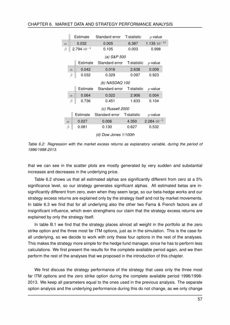
CHAPTER 6. MARKET DATA AND STRATEGY PERFORMANCE ANALYSIS
Estimate Standard error T-statistic p-value
α 0.032 0.005 6.387 1.135·10−19
β 2.794·10−4 0.105 0.003 0.998
(a) S&P 500Estimate Standard error T-statistic p-value
α 0.042 0.016 2.638 0.009β 0.032 0.329 0.097 0.923
(b) NASDAQ 100Estimate Standard error T-statistic p-value
α 0.064 0.022 2.906 0.004β 0.736 0.451 1.633 0.104
(c) Russell 2000Estimate Standard error T-statistic p-value
α 0.027 0.006 4.350 2.284·10−5
β 0.081 0.130 0.627 0.532
(d) Dow Jones 1/100th
Table 6.2: Regression with the market excess returns as explanatory variable, during the period of1996/1998-2013.
that we can see in the scatter plots are mostly generated by very sudden and substantialincreases and decreases in the underlying price.
Table 6.2 shows us that all estimated alphas are significantly different from zero at a 5%significance level, so our strategy generates significant alphas. All estimated betas are in-significantly different from zero, even when they seem large, so our beta-hedge works and ourstrategy excess returns are explained only by the strategy itself and not by market movements.In table 6.3 we find that for all underlying also the other two Fama & French factors are ofinsignificant influence, which even strengthens our claim that the strategy excess returns areexplained by only the strategy itself.
In table B.1 we find that the strategy places almost all weight in the portfolio at the zerostrike option and the three most far ITM options, just as in the simulation. This is the case forall underlying, so we decide to work with only these four options in the rest of the analyses.This makes the strategy more simple for the hedge fund manager, since he has to perform lesscalculations. We first present the results for the complete available period again, and we thenperform the rest of the analyses that we proposed in the introduction of this chapter.
We first discuss the strategy performance of the strategy that uses only the three mostfar ITM options and the zero strike option during the complete available period 1996/1998-2013. We keep all parameters equal to the ones used in the previous analysis. The separateoption analysis and the underlying performance during this do not change, as we only change
57
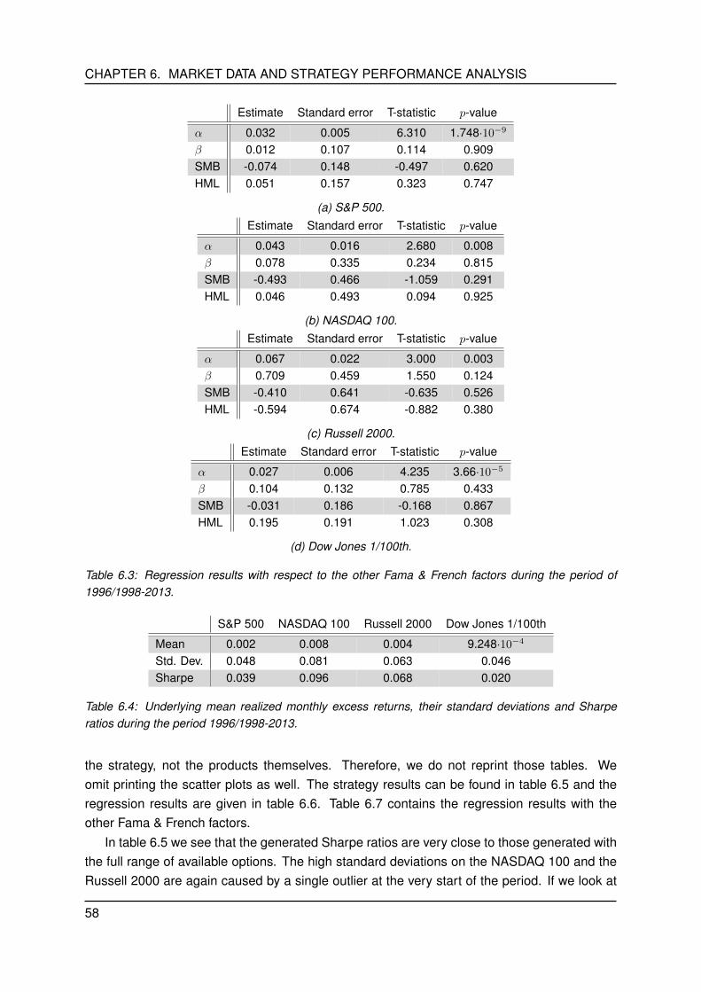
CHAPTER 6. MARKET DATA AND STRATEGY PERFORMANCE ANALYSIS
Estimate Standard error T-statistic p-value
α 0.032 0.005 6.310 1.748·10−9
β 0.012 0.107 0.114 0.909SMB -0.074 0.148 -0.497 0.620HML 0.051 0.157 0.323 0.747
(a) S&P 500.Estimate Standard error T-statistic p-value
α 0.043 0.016 2.680 0.008β 0.078 0.335 0.234 0.815SMB -0.493 0.466 -1.059 0.291HML 0.046 0.493 0.094 0.925
(b) NASDAQ 100.Estimate Standard error T-statistic p-value
α 0.067 0.022 3.000 0.003β 0.709 0.459 1.550 0.124SMB -0.410 0.641 -0.635 0.526HML -0.594 0.674 -0.882 0.380
(c) Russell 2000.Estimate Standard error T-statistic p-value
α 0.027 0.006 4.235 3.66·10−5
β 0.104 0.132 0.785 0.433SMB -0.031 0.186 -0.168 0.867HML 0.195 0.191 1.023 0.308
(d) Dow Jones 1/100th.
Table 6.3: Regression results with respect to the other Fama & French factors during the period of1996/1998-2013.
S&P 500 NASDAQ 100 Russell 2000 Dow Jones 1/100th
Mean 0.002 0.008 0.004 9.248·10−4
Std. Dev. 0.048 0.081 0.063 0.046Sharpe 0.039 0.096 0.068 0.020
Table 6.4: Underlying mean realized monthly excess returns, their standard deviations and Sharperatios during the period 1996/1998-2013.
the strategy, not the products themselves. Therefore, we do not reprint those tables. Weomit printing the scatter plots as well. The strategy results can be found in table 6.5 and theregression results are given in table 6.6. Table 6.7 contains the regression results with theother Fama & French factors.
In table 6.5 we see that the generated Sharpe ratios are very close to those generated withthe full range of available options. The high standard deviations on the NASDAQ 100 and theRussell 2000 are again caused by a single outlier at the very start of the period. If we look at
58
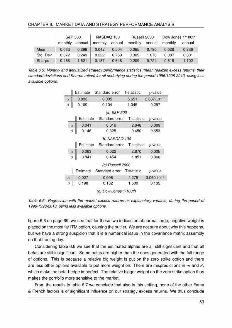
CHAPTER 6. MARKET DATA AND STRATEGY PERFORMANCE ANALYSIS
S&P 500 NASDAQ 100 Russell 2000 Dow Jones 1/100thmonthly annual monthly annual monthly annual monthly annual
Mean 0.033 0.396 0.042 0.504 0.065 0.780 0.028 0.336Std. Dev. 0.072 0.249 0.222 0.769 0.309 1.070 0.087 0.301Sharpe 0.468 1.621 0.187 0.648 0.209 0.724 0.318 1.102
Table 6.5: Monthly and annualized strategy performance statistics (mean realized excess returns, theirstandard deviations and Sharpe ratios) for all underlying during the period 1996/1998-2013, using lessavailable options.
Estimate Standard error T-statistic p-value
α 0.033 0.005 6.651 2.637·10−10
β 0.109 0.104 1.045 0.297
(a) S&P 500Estimate Standard error T-statistic p-value
α 0.041 0.016 2.648 0.009β 0.146 0.325 0.450 0.653
(b) NASDAQ 100Estimate Standard error T-statistic p-value
α 0.063 0.022 2.870 0.005β 0.841 0.454 1.851 0.066
(c) Russell 2000Estimate Standard error T-statistic p-value
α 0.027 0.006 4.278 3.060·10−5
β 0.198 0.132 1.500 0.135
(d) Dow Jones 1/100th
Table 6.6: Regression with the market excess returns as explanatory variable, during the period of1996/1998-2013, using less available options.
figure 6.6 on page 69, we see that for these two indices an abnormal large, negative weight isplaced on the most far ITM option, causing the outlier. We are not sure about why this happens,but we have a strong suspicion that it is a numerical issue in the covariance matrix assemblyon that trading day.
Considering table 6.6 we see that the estimated alphas are all still significant and that allbetas are still insignificant. Some betas are higher than the ones generated with the full rangeof options. This is because a relative big weight is put on the zero strike option and thereare less other options available to put more weight on. There are mispredictions in m and S,which make the beta-hedge imperfect. The relative bigger weight on the zero strike option thusmakes the portfolio more sensitive to the market.
From the results in table 6.7 we conclude that also in this setting, none of the other Fama& French factors is of significant influence on our strategy excess returns. We thus conclude
59

CHAPTER 6. MARKET DATA AND STRATEGY PERFORMANCE ANALYSIS
Estimate Standard error T-statistic p-value
α 0.033 0.005 6.649 2.717·10−10
β 0.125 0.106 1.176 0.241SMB -0.163 0.148 -1.104 0.271HML 0.017 0.156 0.111 0.912
(a) S&P 500.Estimate Standard error T-statistic p-value
α 0.042 0.016 2.693 0.008β 0.189 0.330 0.573 0.567SMB -0.496 0.459 -1.080 0.281HML 0.013 0.486 0.027 0.978
(b) NASDAQ 100.Estimate Standard error T-statistic p-value
α 0.066 0.022 2.958 0.003β 0.808 0.462 1.748 0.082SMB -0.355 0.646 -0.550 0.583HML -0.608 0.680 -0.894 0.372
(c) Russell 2000.Estimate Standard error T-statistic p-value
α 0.027 0.006 4.160 4.965·10−5
β 0.225 0.134 1.682 0.094SMB -0.040 0.188 -0.213 0.832HML 0.239 0.194 1.231 0.220
(d) Dow Jones 1/100th.
Table 6.7: Regression results with respect to the other Fama & French factors during the period of1996/1998-2013, using less available options.
that our strategy still performs well with this smaller range of available options.
We continue with our analysis of strategy performance during our second period of interest;the period running from January 1996/1998 to December 2002, the Dot-com bubble period,giving us 84 observations of excess returns for the S&P 500 and NASDAQ 100, 72 for theRussell 2000 and 60 for the Dow Jones 1/100th. For this period, we again present an analysisof the separate options and the performance of holding the underlying, as well as the strategyperformance results and regressions.
In table B.4 we see that during this period, one generally loses money when one simplyholds an option. Only the the NASDAQ 100 produces positive mean realized option excessreturns. Opposed to the complete timespan, we now find negative expected option excessreturns for every underlying in table B.8.
The strategy performance statistics are found in table 6.8, in which we can see that the
60
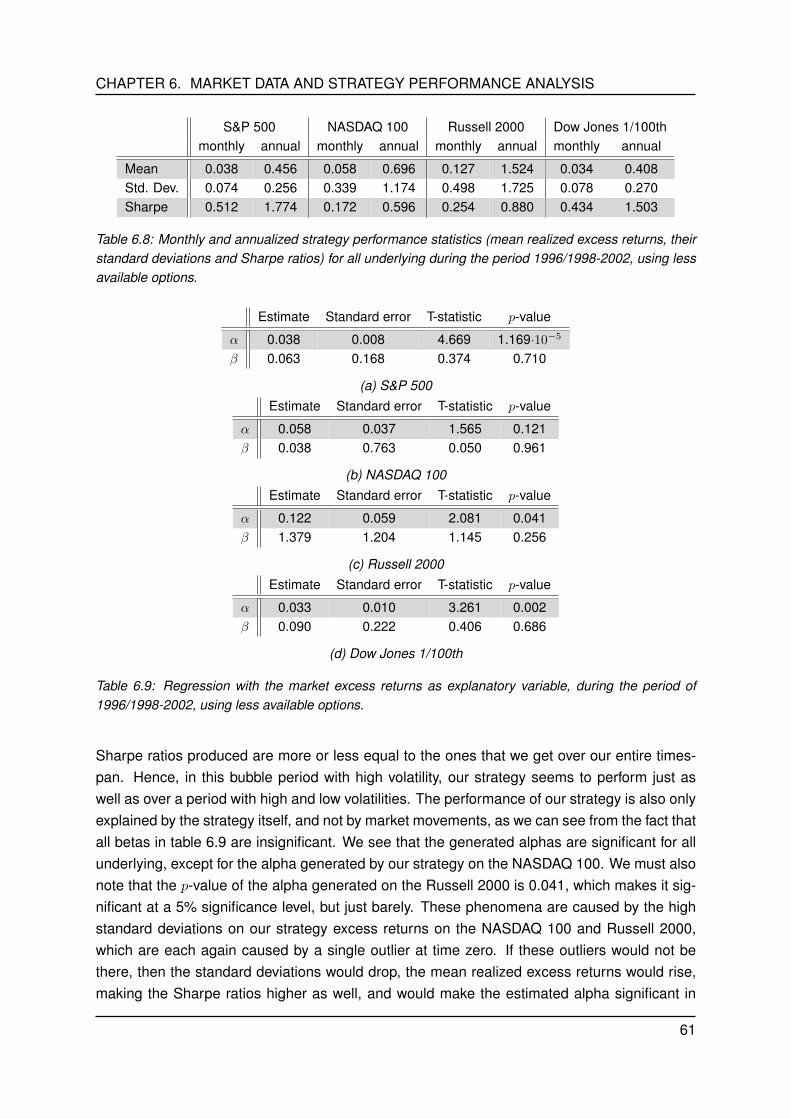
CHAPTER 6. MARKET DATA AND STRATEGY PERFORMANCE ANALYSIS
S&P 500 NASDAQ 100 Russell 2000 Dow Jones 1/100thmonthly annual monthly annual monthly annual monthly annual
Mean 0.038 0.456 0.058 0.696 0.127 1.524 0.034 0.408Std. Dev. 0.074 0.256 0.339 1.174 0.498 1.725 0.078 0.270Sharpe 0.512 1.774 0.172 0.596 0.254 0.880 0.434 1.503
Table 6.8: Monthly and annualized strategy performance statistics (mean realized excess returns, theirstandard deviations and Sharpe ratios) for all underlying during the period 1996/1998-2002, using lessavailable options.
Estimate Standard error T-statistic p-value
α 0.038 0.008 4.669 1.169·10−5
β 0.063 0.168 0.374 0.710
(a) S&P 500Estimate Standard error T-statistic p-value
α 0.058 0.037 1.565 0.121β 0.038 0.763 0.050 0.961
(b) NASDAQ 100Estimate Standard error T-statistic p-value
α 0.122 0.059 2.081 0.041β 1.379 1.204 1.145 0.256
(c) Russell 2000Estimate Standard error T-statistic p-value
α 0.033 0.010 3.261 0.002β 0.090 0.222 0.406 0.686
(d) Dow Jones 1/100th
Table 6.9: Regression with the market excess returns as explanatory variable, during the period of1996/1998-2002, using less available options.
Sharpe ratios produced are more or less equal to the ones that we get over our entire times-pan. Hence, in this bubble period with high volatility, our strategy seems to perform just aswell as over a period with high and low volatilities. The performance of our strategy is also onlyexplained by the strategy itself, and not by market movements, as we can see from the fact thatall betas in table 6.9 are insignificant. We see that the generated alphas are significant for allunderlying, except for the alpha generated by our strategy on the NASDAQ 100. We must alsonote that the p-value of the alpha generated on the Russell 2000 is 0.041, which makes it sig-nificant at a 5% significance level, but just barely. These phenomena are caused by the highstandard deviations on our strategy excess returns on the NASDAQ 100 and Russell 2000,which are each again caused by a single outlier at time zero. If these outliers would not bethere, then the standard deviations would drop, the mean realized excess returns would rise,making the Sharpe ratios higher as well, and would make the estimated alpha significant in
61

CHAPTER 6. MARKET DATA AND STRATEGY PERFORMANCE ANALYSIS
Estimate Standard error T-statistic p-value
α 0.038 0.008 4.504 2.244·10−5
β 0.114 0.217 0.526 0.601SMB -0.003 0.217 -0.015 0.988HML 0.108 0.270 0.399 0.691
(a) S&P 500.Estimate Standard error T-statistic p-value
α 0.058 0.038 1.553 0.124β 0.035 0.784 0.045 0.964SMB -0.250 1.774 -0.141 0.888HML -0.503 1.494 -0.337 0.737
(b) NASDAQ 100.Estimate Standard error T-statistic p-value
α 0.113 0.059 1.901 0.062β 1.298 1.227 1.058 0.294SMB 2.649 2.808 0.943 0.349HML -2.510 2.304 -1.089 0.280
(c) Russell 2000.Estimate Standard error T-statistic p-value
α 0.033 0.011 3.167 0.002β 0.091 0.225 0.403 0.688SMB -0.033 0.465 -0.071 0.943HML -0.245 0.379 -0.647 0.520
(d) Dow Jones 1/100th.
Table 6.10: Regression results with respect to the other Fama & French factors during the period of1996/1998-2002, using less available options.
S&P 500 NASDAQ 100 Russell 2000 Dow Jones 1/100th
Mean -1.091·10−4 0.008 -8.762·10−4 0.003Std. Dev. 0.490 0.108 0.061 0.062Sharpe -0.002 0.077 -0.014 0.041
Table 6.11: Underlying mean realized monthly excess returns, their standard deviations and Sharperatios during the period 1996/1998-2002.
case of the NASDAQ 100. In table 6.10 we see that none of the other Fama & French factors isof significant influence in explaining our strategy excess returns on all of the underlying. If wecompare the underlying performance during this period, given in table 6.11, with our strategyperformance, we see that our strategy generates a higher monthly Sharpe ratio on all of theunderlying than the Sharpe ratios obtained by holding the underlying themselves. Hence, ourstrategy outperforms each benchmark asset during this period, even with the high standarddeviations on the NASDAQ 100 and Russell 2000.
62
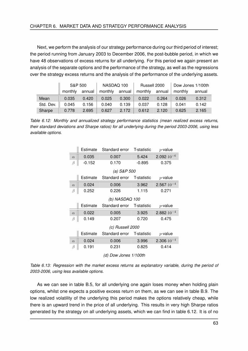
CHAPTER 6. MARKET DATA AND STRATEGY PERFORMANCE ANALYSIS
Next, we perform the analysis of our strategy performance during our third period of interest;the period running from January 2003 to December 2006, the post-bubble period, in which wehave 48 observations of excess returns for all underlying. For this period we again present ananalysis of the separate options and the performance of the strategy, as well as the regressionsover the strategy excess returns and the analysis of the performance of the underlying assets.
S&P 500 NASDAQ 100 Russell 2000 Dow Jones 1/100thmonthly annual monthly annual monthly annual monthly annual
Mean 0.035 0.420 0.025 0.300 0.022 0.264 0.026 0.312Std. Dev. 0.045 0.156 0.040 0.139 0.037 0.128 0.041 0.142Sharpe 0.778 2.695 0.627 2.172 0.612 2.120 0.625 2.165
Table 6.12: Monthly and annualized strategy performance statistics (mean realized excess returns,their standard deviations and Sharpe ratios) for all underlying during the period 2003-2006, using lessavailable options.
Estimate Standard error T-statistic p-value
α 0.035 0.007 5.424 2.092·10−6
β -0.152 0.170 -0.895 0.375
(a) S&P 500Estimate Standard error T-statistic p-value
α 0.024 0.006 3.962 2.567·10−4
β 0.252 0.226 1.115 0.271
(b) NASDAQ 100Estimate Standard error T-statistic p-value
α 0.022 0.005 3.925 2.882·10−4
β 0.149 0.207 0.720 0.475
(c) Russell 2000Estimate Standard error T-statistic p-value
α 0.024 0.006 3.996 2.306·10−4
β 0.191 0.231 0.825 0.414
(d) Dow Jones 1/100th
Table 6.13: Regression with the market excess returns as explanatory variable, during the period of2003-2006, using less available options.
As we can see in table B.5, for all underlying one again loses money when holding plainoptions, whilst one expects a positive excess return on them, as we can see in table B.9. Thelow realized volatility of the underlying this period makes the options relatively cheap, whilethere is an upward trend in the price of all underlying. This results in very high Sharpe ratiosgenerated by the strategy on all underlying assets, which we can find in table 6.12. It is of no
63
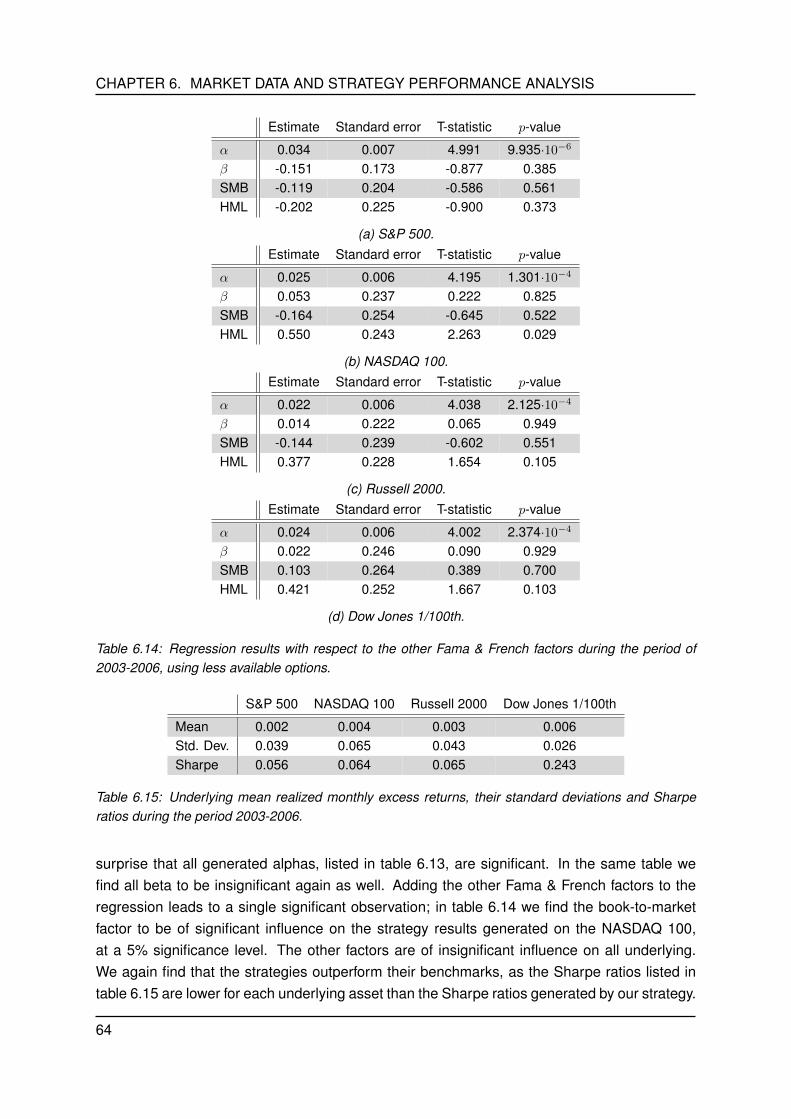
CHAPTER 6. MARKET DATA AND STRATEGY PERFORMANCE ANALYSIS
Estimate Standard error T-statistic p-value
α 0.034 0.007 4.991 9.935·10−6
β -0.151 0.173 -0.877 0.385SMB -0.119 0.204 -0.586 0.561HML -0.202 0.225 -0.900 0.373
(a) S&P 500.Estimate Standard error T-statistic p-value
α 0.025 0.006 4.195 1.301·10−4
β 0.053 0.237 0.222 0.825SMB -0.164 0.254 -0.645 0.522HML 0.550 0.243 2.263 0.029
(b) NASDAQ 100.Estimate Standard error T-statistic p-value
α 0.022 0.006 4.038 2.125·10−4
β 0.014 0.222 0.065 0.949SMB -0.144 0.239 -0.602 0.551HML 0.377 0.228 1.654 0.105
(c) Russell 2000.Estimate Standard error T-statistic p-value
α 0.024 0.006 4.002 2.374·10−4
β 0.022 0.246 0.090 0.929SMB 0.103 0.264 0.389 0.700HML 0.421 0.252 1.667 0.103
(d) Dow Jones 1/100th.
Table 6.14: Regression results with respect to the other Fama & French factors during the period of2003-2006, using less available options.
S&P 500 NASDAQ 100 Russell 2000 Dow Jones 1/100th
Mean 0.002 0.004 0.003 0.006Std. Dev. 0.039 0.065 0.043 0.026Sharpe 0.056 0.064 0.065 0.243
Table 6.15: Underlying mean realized monthly excess returns, their standard deviations and Sharperatios during the period 2003-2006.
surprise that all generated alphas, listed in table 6.13, are significant. In the same table wefind all beta to be insignificant again as well. Adding the other Fama & French factors to theregression leads to a single significant observation; in table 6.14 we find the book-to-marketfactor to be of significant influence on the strategy results generated on the NASDAQ 100,at a 5% significance level. The other factors are of insignificant influence on all underlying.We again find that the strategies outperform their benchmarks, as the Sharpe ratios listed intable 6.15 are lower for each underlying asset than the Sharpe ratios generated by our strategy.
64
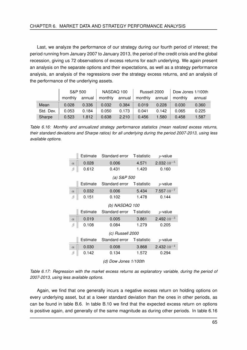
CHAPTER 6. MARKET DATA AND STRATEGY PERFORMANCE ANALYSIS
Last, we analyze the performance of our strategy during our fourth period of interest; theperiod running from January 2007 to January 2013, the period of the credit crisis and the globalrecession, giving us 72 observations of excess returns for each underlying. We again presentan analysis on the separate options and their expectations, as well as a strategy performanceanalysis, an analysis of the regressions over the strategy excess returns, and an analysis ofthe performance of the underlying assets.
S&P 500 NASDAQ 100 Russell 2000 Dow Jones 1/100thmonthly annual monthly annual monthly annual monthly annual
Mean 0.028 0.336 0.032 0.384 0.019 0.228 0.030 0.360Std. Dev. 0.053 0.184 0.050 0.173 0.041 0.142 0.065 0.225Sharpe 0.523 1.812 0.638 2.210 0.456 1.580 0.458 1.587
Table 6.16: Monthly and annualized strategy performance statistics (mean realized excess returns,their standard deviations and Sharpe ratios) for all underlying during the period 2007-2013, using lessavailable options.
Estimate Standard error T-statistic p-value
α 0.028 0.006 4.571 2.032·10−5
β 0.612 0.431 1.420 0.160
(a) S&P 500Estimate Standard error T-statistic p-value
α 0.032 0.006 5.434 7.557·10−7
β 0.151 0.102 1.478 0.144
(b) NASDAQ 100Estimate Standard error T-statistic p-value
α 0.019 0.005 3.861 2.492·10−3
β 0.108 0.084 1.279 0.205
(c) Russell 2000Estimate Standard error T-statistic p-value
α 0.030 0.008 3.868 2.432·10−4
β 0.142 0.134 1.572 0.294
(d) Dow Jones 1/100th
Table 6.17: Regression with the market excess returns as explanatory variable, during the period of2007-2013, using less available options.
Again, we find that one generally incurs a negative excess return on holding options onevery underlying asset, but at a lower standard deviation than the ones in other periods, ascan be found in table B.6. In table B.10 we find that the expected excess return on optionsis positive again, and generally of the same magnitude as during other periods. In table 6.16
65
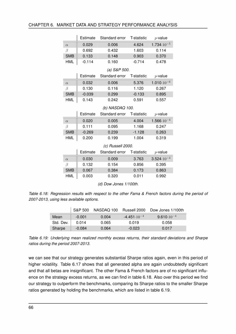
CHAPTER 6. MARKET DATA AND STRATEGY PERFORMANCE ANALYSIS
Estimate Standard error T-statistic p-value
α 0.029 0.006 4.624 1.734·10−5
β 0.692 0.432 1.603 0.114SMB 0.133 0.148 0.903 0.370HML -0.114 0.160 -0.714 0.478
(a) S&P 500.Estimate Standard error T-statistic p-value
α 0.032 0.006 5.376 1.010·10−6
β 0.130 0.116 1.120 0.267SMB -0.039 0.299 -0.133 0.895HML 0.143 0.242 0.591 0.557
(b) NASDAQ 100.Estimate Standard error T-statistic p-value
α 0.020 0.005 4.004 1.566·10−4
β 0.111 0.095 1.168 0.247SMB -0.269 0.239 -1.128 0.263HML 0.200 0.199 1.004 0.319
(c) Russell 2000.Estimate Standard error T-statistic p-value
α 0.030 0.009 3.763 3.524·10−4
β 0.132 0.154 0.856 0.395SMB 0.067 0.384 0.173 0.863HML 0.003 0.320 0.011 0.992
(d) Dow Jones 1/100th.
Table 6.18: Regression results with respect to the other Fama & French factors during the period of2007-2013, using less available options.
S&P 500 NASDAQ 100 Russell 2000 Dow Jones 1/100th
Mean -0.001 0.004 -4.451·10−4 9.610·10−4
Std. Dev. 0.014 0.065 0.019 0.058Sharpe -0.084 0.064 -0.023 0.017
Table 6.19: Underlying mean realized monthly excess returns, their standard deviations and Sharperatios during the period 2007-2013.
we can see that our strategy generates substantial Sharpe ratios again, even in this period ofhigher volatility. Table 6.17 shows that all generated alpha are again undoubtedly significantand that all betas are insignificant. The other Fama & French factors are of no significant influ-ence on the strategy excess returns, as we can find in table 6.18. Also over this period we findour strategy to outperform the benchmarks, comparing its Sharpe ratios to the smaller Sharperatios generated by holding the benchmarks, which are listed in table 6.19.
66
CHAPTER 6. MARKET DATA AND STRATEGY PERFORMANCE ANALYSIS
Considering the analysis of our strategy performance during the four periods, we concludethat our strategy performs well, as it generates substantial Sharpe ratios and outperforms hold-ing the benchmarks in every period. As all generated betas in all periods are insignificantlydifferent from zero at a 5% significance level, we conclude that the generated excess returnsby the strategy are all explained by only the strategy itself, and their alphas to be significantlydifferent from zero at a 5% significance level (except for the one on the NASDAQ 100 during2003-2006 as result of a numerical error). In almost all cases we find the other Fama & Frenchfactors to be insignificant in the regression as well, which strengthens our claim of that thestrategy excess returns are solely explained by the strategy itself. We note that the standarddeviation of the excess returns generated by the strategy is sometimes far from 5% per month,mostly due to a single outlier, of which the cause cannot be explained by market crashes, etc,but is more likely to be generated by numerical issues in the analysis. When we compareour obtained Sharpe ratios with Sharpe ratios of previous research, they look good as well.Eraker [3] reports Sharpe ratios near one in yearly figures for portfolios with short positions incall options on the S&P 500 during the period 1996-2013 and Kapadia and Szado [5] reportmonthly Sharpe ratios between 0.130 and 0.160 on buy-write strategies with call options onthe Russell 2000 during the period 1996-2006, but we do note that they use other models andperiods of time for their analyses, so we cannot easily compare the results, but we do get anidea of the magnitude of Sharpe ratios found in previous research. Therefore, we concludethat our strategy generally performs outstanding in this one dimensional setting during thesehistorical periods, even with the assumption of a fixed growth rate µ and the assumption thatthe underlying has a beta with respect to the market of one.
We now study whether the results improve when one uses a market beta unequal to one.As we use a more realistic beta, we expect that the estimated beta obtained in the regression(1.1) will be closer to zero, especially in the case where we update βmkt dynamically with theextra information available on the market every next trading day. We perform this analysisover the period of January 2001 - January 2013 (resulting in 145 observations of strategy andmarket excess returns), as this enables us to use data from the Optionmetrics database in theperiods prior to our first trade. For each underlying we choose the period to be the period fromwhen we first have data on the underlying to December 2000, hence, for the NASDAQ 100this is 1996-2000, for the Russell 2000 this is 1997-2000 and for the Dow Jones 1/100th thisis 1998-2000. In this analysis we use the same parameters as in our previous analyses, andwe work with the three most far ITM options and the zero strike option available in our portfolioselection.
In table 6.20 we list the results of the analysis; for every asset we present the mean monthlystrategy excess return, its standard deviation, its Sharpe ratio, and the estimated alpha andbeta in the regression (1.1). In the first column we present the results with a market beta equalto one, as a reference. In the second column we present the results generated with a fixedmarket beta, calculated over the period prior to our first trade. In the last column we list theresults generated with a dynamically updated market beta. All the reported alphas are sig-
67
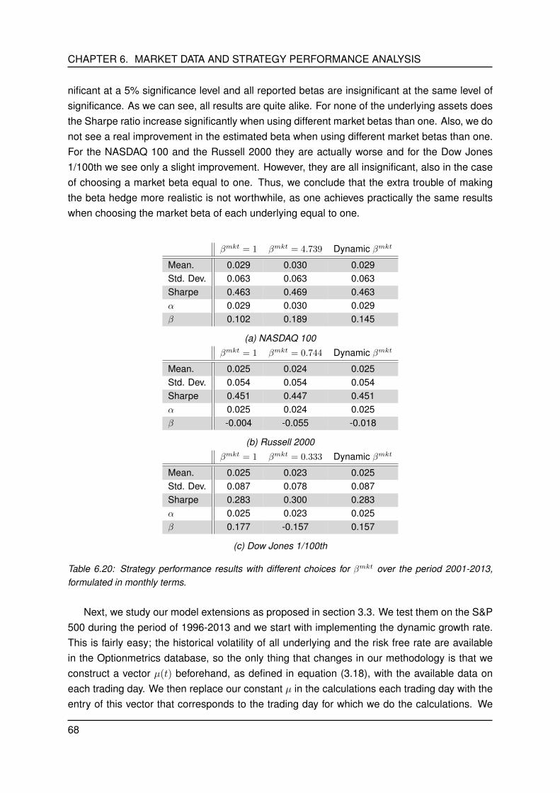
CHAPTER 6. MARKET DATA AND STRATEGY PERFORMANCE ANALYSIS
nificant at a 5% significance level and all reported betas are insignificant at the same level ofsignificance. As we can see, all results are quite alike. For none of the underlying assets doesthe Sharpe ratio increase significantly when using different market betas than one. Also, we donot see a real improvement in the estimated beta when using different market betas than one.For the NASDAQ 100 and the Russell 2000 they are actually worse and for the Dow Jones1/100th we see only a slight improvement. However, they are all insignificant, also in the caseof choosing a market beta equal to one. Thus, we conclude that the extra trouble of makingthe beta hedge more realistic is not worthwhile, as one achieves practically the same resultswhen choosing the market beta of each underlying equal to one.
βmkt = 1 βmkt = 4.739 Dynamic βmkt
Mean. 0.029 0.030 0.029Std. Dev. 0.063 0.063 0.063Sharpe 0.463 0.469 0.463α 0.029 0.030 0.029β 0.102 0.189 0.145
(a) NASDAQ 100βmkt = 1 βmkt = 0.744 Dynamic βmkt
Mean. 0.025 0.024 0.025Std. Dev. 0.054 0.054 0.054Sharpe 0.451 0.447 0.451α 0.025 0.024 0.025β -0.004 -0.055 -0.018
(b) Russell 2000βmkt = 1 βmkt = 0.333 Dynamic βmkt
Mean. 0.025 0.023 0.025Std. Dev. 0.087 0.078 0.087Sharpe 0.283 0.300 0.283α 0.025 0.023 0.025β 0.177 -0.157 0.157
(c) Dow Jones 1/100th
Table 6.20: Strategy performance results with different choices for βmkt over the period 2001-2013,formulated in monthly terms.
Next, we study our model extensions as proposed in section 3.3. We test them on the S&P500 during the period of 1996-2013 and we start with implementing the dynamic growth rate.This is fairly easy; the historical volatility of all underlying and the risk free rate are availablein the Optionmetrics database, so the only thing that changes in our methodology is that weconstruct a vector µ(t) beforehand, as defined in equation (3.18), with the available data oneach trading day. We then replace our constant µ in the calculations each trading day with theentry of this vector that corresponds to the trading day for which we do the calculations. We
68
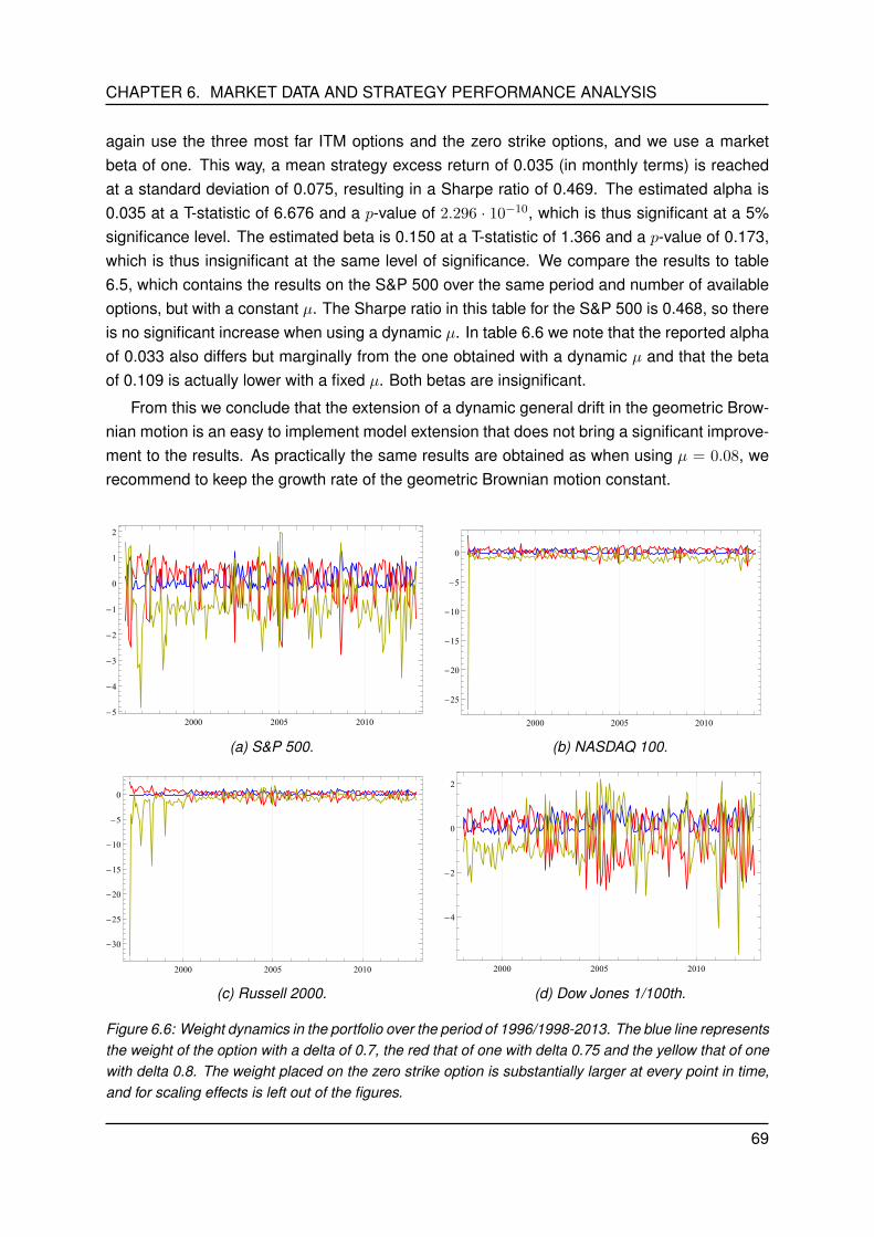
CHAPTER 6. MARKET DATA AND STRATEGY PERFORMANCE ANALYSIS
again use the three most far ITM options and the zero strike options, and we use a marketbeta of one. This way, a mean strategy excess return of 0.035 (in monthly terms) is reachedat a standard deviation of 0.075, resulting in a Sharpe ratio of 0.469. The estimated alpha is0.035 at a T-statistic of 6.676 and a p-value of 2.296 · 10−10, which is thus significant at a 5%significance level. The estimated beta is 0.150 at a T-statistic of 1.366 and a p-value of 0.173,which is thus insignificant at the same level of significance. We compare the results to table6.5, which contains the results on the S&P 500 over the same period and number of availableoptions, but with a constant µ. The Sharpe ratio in this table for the S&P 500 is 0.468, so thereis no significant increase when using a dynamic µ. In table 6.6 we note that the reported alphaof 0.033 also differs but marginally from the one obtained with a dynamic µ and that the betaof 0.109 is actually lower with a fixed µ. Both betas are insignificant.
From this we conclude that the extension of a dynamic general drift in the geometric Brow-nian motion is an easy to implement model extension that does not bring a significant improve-ment to the results. As practically the same results are obtained as when using µ = 0.08, werecommend to keep the growth rate of the geometric Brownian motion constant.
2000 2005 2010-5
-4
-3
-2
-1
0
1
2
(a) S&P 500.
2000 2005 2010
-25
-20
-15
-10
-5
0
(b) NASDAQ 100.
2000 2005 2010
-30
-25
-20
-15
-10
-5
0
(c) Russell 2000.
2000 2005 2010
-4
-2
0
2
(d) Dow Jones 1/100th.
Figure 6.6: Weight dynamics in the portfolio over the period of 1996/1998-2013. The blue line representsthe weight of the option with a delta of 0.7, the red that of one with delta 0.75 and the yellow that of onewith delta 0.8. The weight placed on the zero strike option is substantially larger at every point in time,and for scaling effects is left out of the figures.
69

CHAPTER 6. MARKET DATA AND STRATEGY PERFORMANCE ANALYSIS
The second, and last, model extension we suggested, was to implement trading costs inan easy fashion. If the strategy would constantly buy one type of option and would sell an-other, then we could adjust the prices of these products in hindsight and perform the analysesagain. However, when we look at figure 6.6, which describes the weight dynamics of the port-folio through time (with constant µ, βmkt = 1 and only the most far ITM and the zero strikeoptions available, over the period of 1996/1998-2013), we can see that for every underlying notype of option is solely bought or shorted in the period. The other investigated periods showsimilar dynamics, so unfortunately, we cannot simply implement the trading costs in the waywe suggested. Implementing them otherwise is beyond the scope of this thesis, but we dorecommend this addition for further research.
6.3 Strategy performance analysis with multiple benchmark as-sets
In this section we study the performance of our derived strategy for the multidimensional casewith historical market data. We perform the analyses in a two dimensional setting with theS&P 500 and the Russell 2000 as underlying assets, in which we again use the S&P 500 as arepresentative of the market itself. We first elaborate on our methodology and we then performour analyses during the same periods as in the previous section, but with a slight alterationto the first and second periods; since we now need data available on both underlying, we willlet the first trading day be January 3rd 2000. As we have concluded in the previous sessionthat the results do not improve with a dynamic µ or a market beta unequal to one, so wekeep µ constant for both assets and the market beta equal to one. We elaborate on thestrategy performance in a same kind of way as in the previous section and we again presentthe estimated alpha and beta in the regression (1.1), as well as the regression with the otherFama & French factors. We then compare the results obtained with our strategy to a naivestrategy that divides ones wealth in two equal parts and uses each part to invest on a singleunderlying asset with our one dimensional strategy. If our multidimensional strategy workswell, we expect to see an increase in the Sharpe ratio with respect to this naive strategy. Wealso test our strategy on two combinations of three separate assets in the Dow Jones indexover the period of January 2001 to January 2013; we consider the Walt Disney Corporation,the McDonald’s Corporation and Walmart Stores Incorporated, which are the three of the bestperforming assets in the Dow Jones index. The tables on individual option analysis can befound in Appendix B.
6.3.1 Methodology
Our methodology in this case is a lot like the one in the singe underlying case of the previoussection and the one used in the simulations in section 5.2. We again trade on every firstbusiness day of the month. We assume both underlying follow a geometric Brownian motion
70
CHAPTER 6. MARKET DATA AND STRATEGY PERFORMANCE ANALYSIS
with µ1 = µ2 = 0.08, where we use 1 to refer to the S&P 500 and 2 to refer to the Russell2000, and for σ1 and σ2 we use the observed realized volatilities on the S&P 500 and theRussell 2000 respectively on each trading day. We determine the correlation between the twogeometric Brownian motions by taking the daily log returns on both assets during a period priorto our first trade and compute the correlation between them. We keep this correlation constantthroughout the whole analysis. One could calculate this correlation dynamically each tradingday, based on a fixed period prior to the trading day, but whilst experimenting with this, we raninto numerical issues with the covariance matrix, so we chose to keep it constant.
We again use the monthly observed closing prices of the indices for S(i)t and S(i)
T , i = 1, 2,and we consider the same 13 standardized European call options available on each tradingday for each of the underlying available in the Optionmetrics database, and add the zero strikeoption. Each option has an expiry of 30 days, so ∆t = 1/12. We construct the vector S(i)
T
for both assets in the same way as in the one dimensional case and we calculate the realizedexcess return on all options and the underlying themselves for each trading day, using themarket data of prices, volatilities and interest rates. We combine the realized excess returnson options and the underlying themselves again in vectors, as in the simulations of section 5.2.
We then compute the entries of m and S as in section 4.1 and assemble them for everytrading day. We then assemble our portfolio each trading day with weights given by Theorem4.1.2. To prevent overcompensation in the hedging effect, we generally only hedge with respectto the S&P 500 (or in the case of the Dow Jones single components; we shall only hedge withrespect to one of the assets). In this case, βmkt1 is obviously equal to one and βmkt2 is left outof the equation.
We then compute the realized excess return that follows from the portfolio choice eachtrading day by multiplying the weights and the realized excess returns vector, collect them ina vector Rpf and then compute the mean excess return, its standard deviation and its Sharperatio. Then we perform the regressions with the market excess returns as explanatory variableand the complete set of Fama & French factors as explanatory variables, to see whether theregression alphas are significantly different from zero and the regression betas insignificantlydifferent from zero. We again always use a significance level of 5%, unless we mention other-wise.
When using the Dow Jones single components there is one minor adjustment to the method-ology; thus far we have worked with actual closing prices on the underlying, as there were noreported splits and dividends in the Optionmetrics database for the underlying indices, how-ever, these phenomena do occur with the single components of the Dow Jones. Therefore,we first adjust the closing prices of these stocks and the option prices and strikes for splits.Usually stock option prices are not adjusted for cash settled dividends of less than 10%, so wedo not adjust for dividends.
The methodology of our naive strategy is simple; for the same period we calculate theexcess returns generated by our one dimensional strategy on each underlying. On each trading
71
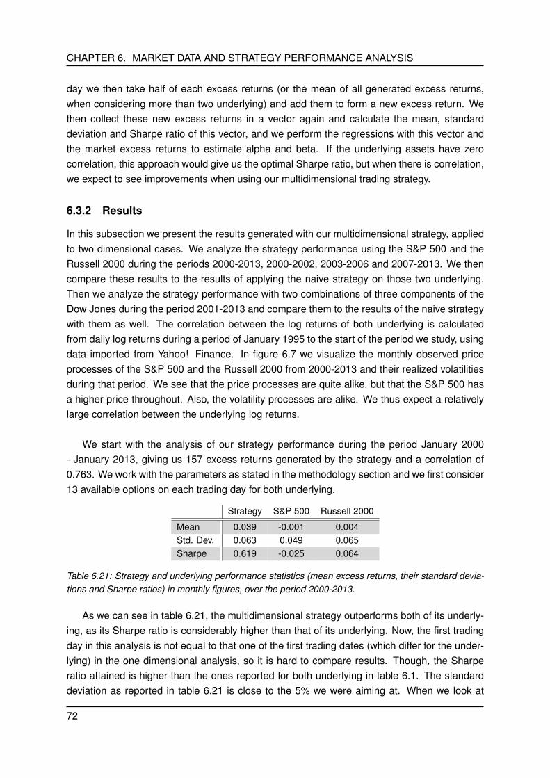
CHAPTER 6. MARKET DATA AND STRATEGY PERFORMANCE ANALYSIS
day we then take half of each excess returns (or the mean of all generated excess returns,when considering more than two underlying) and add them to form a new excess return. Wethen collect these new excess returns in a vector again and calculate the mean, standarddeviation and Sharpe ratio of this vector, and we perform the regressions with this vector andthe market excess returns to estimate alpha and beta. If the underlying assets have zerocorrelation, this approach would give us the optimal Sharpe ratio, but when there is correlation,we expect to see improvements when using our multidimensional trading strategy.
6.3.2 Results
In this subsection we present the results generated with our multidimensional strategy, appliedto two dimensional cases. We analyze the strategy performance using the S&P 500 and theRussell 2000 during the periods 2000-2013, 2000-2002, 2003-2006 and 2007-2013. We thencompare these results to the results of applying the naive strategy on those two underlying.Then we analyze the strategy performance with two combinations of three components of theDow Jones during the period 2001-2013 and compare them to the results of the naive strategywith them as well. The correlation between the log returns of both underlying is calculatedfrom daily log returns during a period of January 1995 to the start of the period we study, usingdata imported from Yahoo! Finance. In figure 6.7 we visualize the monthly observed priceprocesses of the S&P 500 and the Russell 2000 from 2000-2013 and their realized volatilitiesduring that period. We see that the price processes are quite alike, but that the S&P 500 hasa higher price throughout. Also, the volatility processes are alike. We thus expect a relativelylarge correlation between the underlying log returns.
We start with the analysis of our strategy performance during the period January 2000- January 2013, giving us 157 excess returns generated by the strategy and a correlation of0.763. We work with the parameters as stated in the methodology section and we first consider13 available options on each trading day for both underlying.
Strategy S&P 500 Russell 2000
Mean 0.039 -0.001 0.004Std. Dev. 0.063 0.049 0.065Sharpe 0.619 -0.025 0.064
Table 6.21: Strategy and underlying performance statistics (mean excess returns, their standard devia-tions and Sharpe ratios) in monthly figures, over the period 2000-2013.
As we can see in table 6.21, the multidimensional strategy outperforms both of its underly-ing, as its Sharpe ratio is considerably higher than that of its underlying. Now, the first tradingday in this analysis is not equal to that one of the first trading dates (which differ for the under-lying) in the one dimensional analysis, so it is hard to compare results. Though, the Sharperatio attained is higher than the ones reported for both underlying in table 6.1. The standarddeviation as reported in table 6.21 is close to the 5% we were aiming at. When we look at
72

CHAPTER 6. MARKET DATA AND STRATEGY PERFORMANCE ANALYSIS
2000 2005 2010
400
600
800
1000
1200
1400
(a) Price processes.
2000 2005 2010
0.2
0.4
0.6
0.8
(b) Realized volatilities.
Figure 6.7: The monthly price processes of the S&P 500 and the Russell 2000 during the period 2000-2013 and their realized volatilities. The blue lines are those of the S&P 500 and the red lines are thoseof the Russell 2000.
Estimate Standard error T-statistic p-value
α 0.039 0.005 7.747 1.153·10−12
β -0.145 0.104 -1.394 0.165
Table 6.22: Regression with the market excess returns as explanatory variable, during the period of2000-2013.
table 6.22, we can see that the estimated alpha is significant at a 5% significance level andthat the estimated beta of the market excess returns is insignificant at this significance level.In table 6.23 we find that none of the other Fama & French factors are of significant influenceon the strategy excess returns. When one studies the strategy performance when hedging on
73
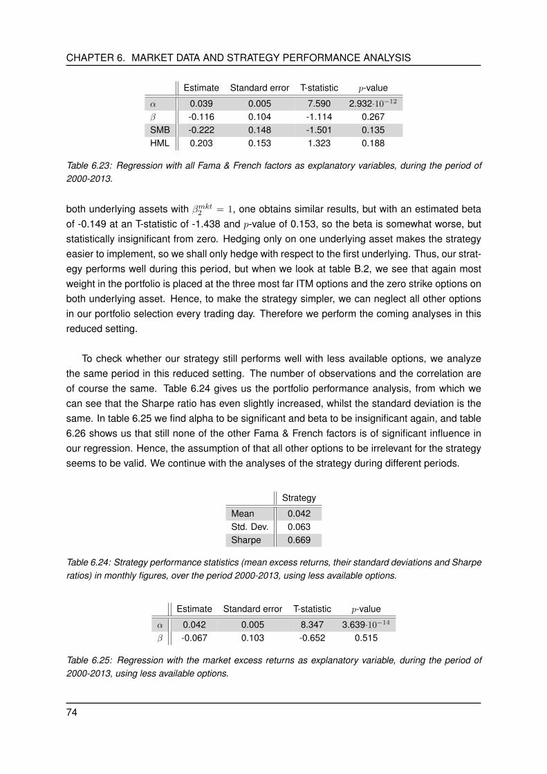
CHAPTER 6. MARKET DATA AND STRATEGY PERFORMANCE ANALYSIS
Estimate Standard error T-statistic p-value
α 0.039 0.005 7.590 2.932·10−12
β -0.116 0.104 -1.114 0.267SMB -0.222 0.148 -1.501 0.135HML 0.203 0.153 1.323 0.188
Table 6.23: Regression with all Fama & French factors as explanatory variables, during the period of2000-2013.
both underlying assets with βmkt2 = 1, one obtains similar results, but with an estimated betaof -0.149 at an T-statistic of -1.438 and p-value of 0.153, so the beta is somewhat worse, butstatistically insignificant from zero. Hedging only on one underlying asset makes the strategyeasier to implement, so we shall only hedge with respect to the first underlying. Thus, our strat-egy performs well during this period, but when we look at table B.2, we see that again mostweight in the portfolio is placed at the three most far ITM options and the zero strike options onboth underlying asset. Hence, to make the strategy simpler, we can neglect all other optionsin our portfolio selection every trading day. Therefore we perform the coming analyses in thisreduced setting.
To check whether our strategy still performs well with less available options, we analyzethe same period in this reduced setting. The number of observations and the correlation areof course the same. Table 6.24 gives us the portfolio performance analysis, from which wecan see that the Sharpe ratio has even slightly increased, whilst the standard deviation is thesame. In table 6.25 we find alpha to be significant and beta to be insignificant again, and table6.26 shows us that still none of the other Fama & French factors is of significant influence inour regression. Hence, the assumption of that all other options to be irrelevant for the strategyseems to be valid. We continue with the analyses of the strategy during different periods.
Strategy
Mean 0.042Std. Dev. 0.063Sharpe 0.669
Table 6.24: Strategy performance statistics (mean excess returns, their standard deviations and Sharperatios) in monthly figures, over the period 2000-2013, using less available options.
Estimate Standard error T-statistic p-value
α 0.042 0.005 8.347 3.639·10−14
β -0.067 0.103 -0.652 0.515
Table 6.25: Regression with the market excess returns as explanatory variable, during the period of2000-2013, using less available options.
74
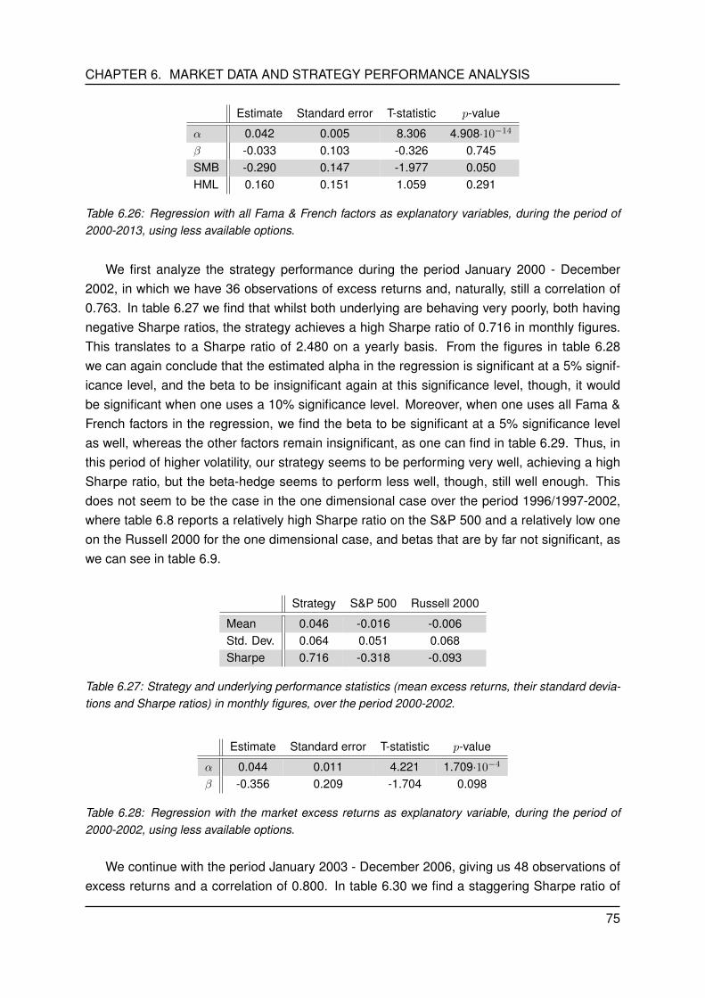
CHAPTER 6. MARKET DATA AND STRATEGY PERFORMANCE ANALYSIS
Estimate Standard error T-statistic p-value
α 0.042 0.005 8.306 4.908·10−14
β -0.033 0.103 -0.326 0.745SMB -0.290 0.147 -1.977 0.050HML 0.160 0.151 1.059 0.291
Table 6.26: Regression with all Fama & French factors as explanatory variables, during the period of2000-2013, using less available options.
We first analyze the strategy performance during the period January 2000 - December2002, in which we have 36 observations of excess returns and, naturally, still a correlation of0.763. In table 6.27 we find that whilst both underlying are behaving very poorly, both havingnegative Sharpe ratios, the strategy achieves a high Sharpe ratio of 0.716 in monthly figures.This translates to a Sharpe ratio of 2.480 on a yearly basis. From the figures in table 6.28we can again conclude that the estimated alpha in the regression is significant at a 5% signif-icance level, and the beta to be insignificant again at this significance level, though, it wouldbe significant when one uses a 10% significance level. Moreover, when one uses all Fama &French factors in the regression, we find the beta to be significant at a 5% significance levelas well, whereas the other factors remain insignificant, as one can find in table 6.29. Thus, inthis period of higher volatility, our strategy seems to be performing very well, achieving a highSharpe ratio, but the beta-hedge seems to perform less well, though, still well enough. Thisdoes not seem to be the case in the one dimensional case over the period 1996/1997-2002,where table 6.8 reports a relatively high Sharpe ratio on the S&P 500 and a relatively low oneon the Russell 2000 for the one dimensional case, and betas that are by far not significant, aswe can see in table 6.9.
Strategy S&P 500 Russell 2000
Mean 0.046 -0.016 -0.006Std. Dev. 0.064 0.051 0.068Sharpe 0.716 -0.318 -0.093
Table 6.27: Strategy and underlying performance statistics (mean excess returns, their standard devia-tions and Sharpe ratios) in monthly figures, over the period 2000-2002.
Estimate Standard error T-statistic p-value
α 0.044 0.011 4.221 1.709·10−4
β -0.356 0.209 -1.704 0.098
Table 6.28: Regression with the market excess returns as explanatory variable, during the period of2000-2002, using less available options.
We continue with the period January 2003 - December 2006, giving us 48 observations ofexcess returns and a correlation of 0.800. In table 6.30 we find a staggering Sharpe ratio of
75
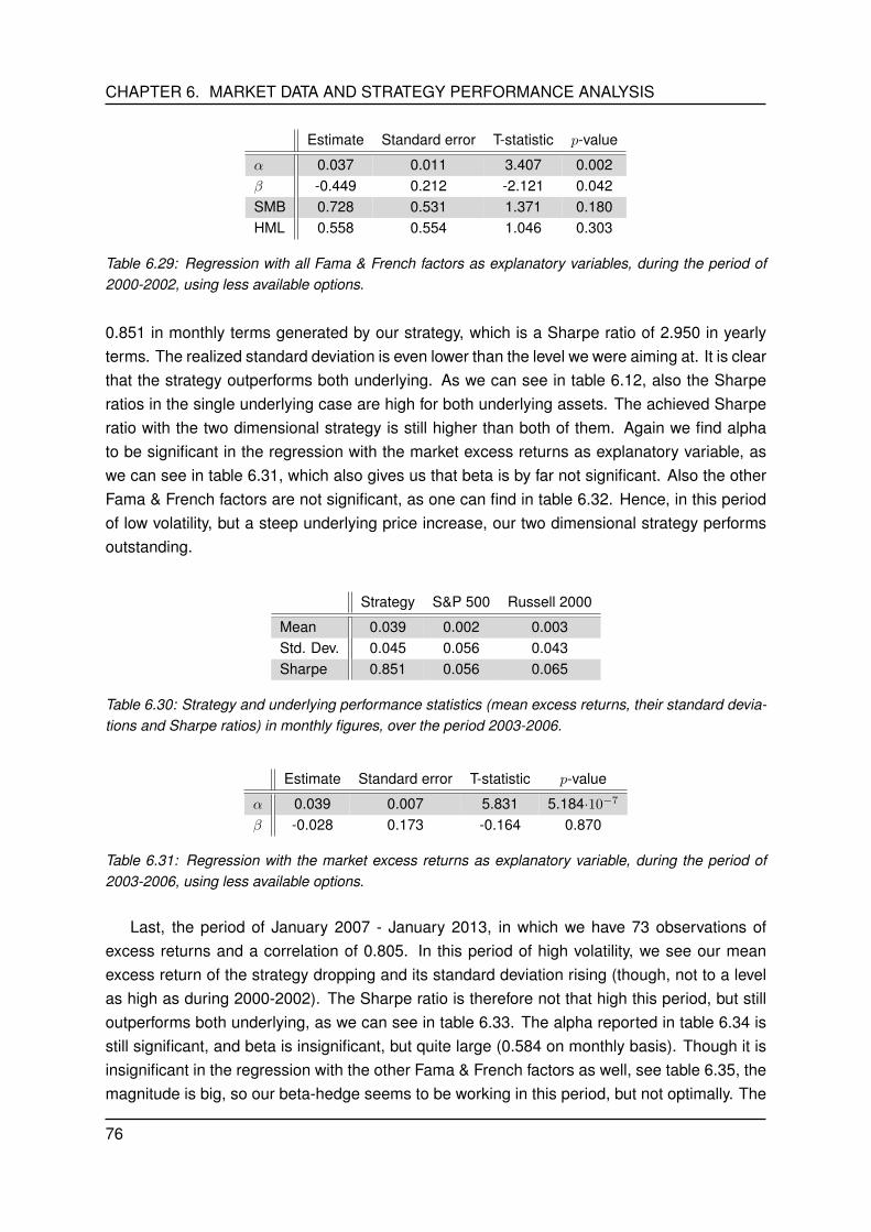
CHAPTER 6. MARKET DATA AND STRATEGY PERFORMANCE ANALYSIS
Estimate Standard error T-statistic p-value
α 0.037 0.011 3.407 0.002β -0.449 0.212 -2.121 0.042SMB 0.728 0.531 1.371 0.180HML 0.558 0.554 1.046 0.303
Table 6.29: Regression with all Fama & French factors as explanatory variables, during the period of2000-2002, using less available options.
0.851 in monthly terms generated by our strategy, which is a Sharpe ratio of 2.950 in yearlyterms. The realized standard deviation is even lower than the level we were aiming at. It is clearthat the strategy outperforms both underlying. As we can see in table 6.12, also the Sharperatios in the single underlying case are high for both underlying assets. The achieved Sharperatio with the two dimensional strategy is still higher than both of them. Again we find alphato be significant in the regression with the market excess returns as explanatory variable, aswe can see in table 6.31, which also gives us that beta is by far not significant. Also the otherFama & French factors are not significant, as one can find in table 6.32. Hence, in this periodof low volatility, but a steep underlying price increase, our two dimensional strategy performsoutstanding.
Strategy S&P 500 Russell 2000
Mean 0.039 0.002 0.003Std. Dev. 0.045 0.056 0.043Sharpe 0.851 0.056 0.065
Table 6.30: Strategy and underlying performance statistics (mean excess returns, their standard devia-tions and Sharpe ratios) in monthly figures, over the period 2003-2006.
Estimate Standard error T-statistic p-value
α 0.039 0.007 5.831 5.184·10−7
β -0.028 0.173 -0.164 0.870
Table 6.31: Regression with the market excess returns as explanatory variable, during the period of2003-2006, using less available options.
Last, the period of January 2007 - January 2013, in which we have 73 observations ofexcess returns and a correlation of 0.805. In this period of high volatility, we see our meanexcess return of the strategy dropping and its standard deviation rising (though, not to a levelas high as during 2000-2002). The Sharpe ratio is therefore not that high this period, but stilloutperforms both underlying, as we can see in table 6.33. The alpha reported in table 6.34 isstill significant, and beta is insignificant, but quite large (0.584 on monthly basis). Though it isinsignificant in the regression with the other Fama & French factors as well, see table 6.35, themagnitude is big, so our beta-hedge seems to be working in this period, but not optimally. The
76
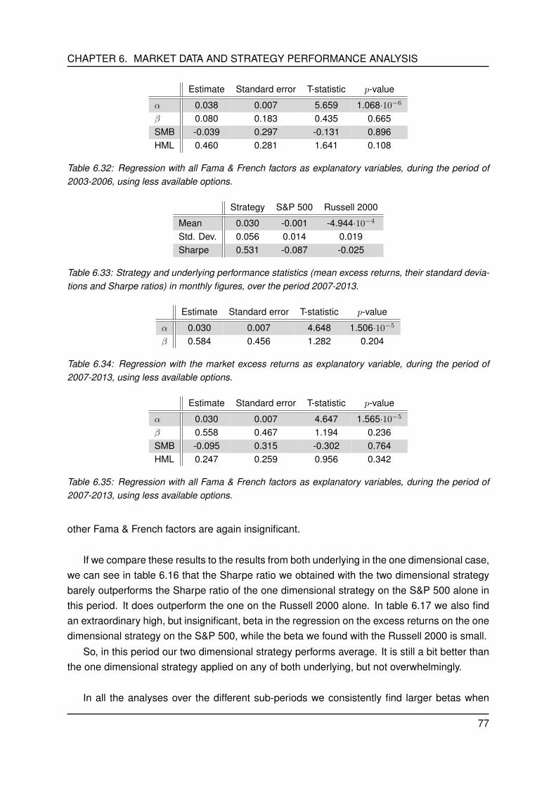
CHAPTER 6. MARKET DATA AND STRATEGY PERFORMANCE ANALYSIS
Estimate Standard error T-statistic p-value
α 0.038 0.007 5.659 1.068·10−6
β 0.080 0.183 0.435 0.665SMB -0.039 0.297 -0.131 0.896HML 0.460 0.281 1.641 0.108
Table 6.32: Regression with all Fama & French factors as explanatory variables, during the period of2003-2006, using less available options.
Strategy S&P 500 Russell 2000
Mean 0.030 -0.001 -4.944·10−4
Std. Dev. 0.056 0.014 0.019Sharpe 0.531 -0.087 -0.025
Table 6.33: Strategy and underlying performance statistics (mean excess returns, their standard devia-tions and Sharpe ratios) in monthly figures, over the period 2007-2013.
Estimate Standard error T-statistic p-value
α 0.030 0.007 4.648 1.506·10−5
β 0.584 0.456 1.282 0.204
Table 6.34: Regression with the market excess returns as explanatory variable, during the period of2007-2013, using less available options.
Estimate Standard error T-statistic p-value
α 0.030 0.007 4.647 1.565·10−5
β 0.558 0.467 1.194 0.236SMB -0.095 0.315 -0.302 0.764HML 0.247 0.259 0.956 0.342
Table 6.35: Regression with all Fama & French factors as explanatory variables, during the period of2007-2013, using less available options.
other Fama & French factors are again insignificant.
If we compare these results to the results from both underlying in the one dimensional case,we can see in table 6.16 that the Sharpe ratio we obtained with the two dimensional strategybarely outperforms the Sharpe ratio of the one dimensional strategy on the S&P 500 alone inthis period. It does outperform the one on the Russell 2000 alone. In table 6.17 we also findan extraordinary high, but insignificant, beta in the regression on the excess returns on the onedimensional strategy on the S&P 500, while the beta we found with the Russell 2000 is small.
So, in this period our two dimensional strategy performs average. It is still a bit better thanthe one dimensional strategy applied on any of both underlying, but not overwhelmingly.
In all the analyses over the different sub-periods we consistently find larger betas when
77
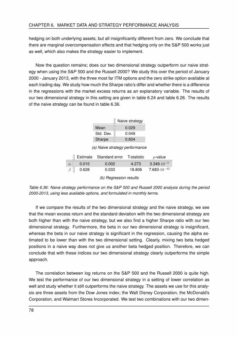
CHAPTER 6. MARKET DATA AND STRATEGY PERFORMANCE ANALYSIS
hedging on both underlying assets, but all insignificantly different from zero. We conclude thatthere are marginal overcompensation effects and that hedging only on the S&P 500 works justas well, which also makes the strategy easier to implement.
Now the question remains; does our two dimensional strategy outperform our naive strat-egy when using the S&P 500 and the Russell 2000? We study this over the period of January2000 - January 2013, with the three most far ITM options and the zero strike option available ateach trading day. We study how much the Sharpe ratio’s differ and whether there is a differencein the regressions with the market excess returns as an explanatory variable. The results ofour two dimensional strategy in this setting are given in table 6.24 and table 6.26. The resultsof the naive strategy can be found in table 6.36.
Naive strategy
Mean 0.029Std. Dev. 0.049Sharpe 0.604
(a) Naive strategy performance
Estimate Standard error T-statistic p-value
α 0.010 0.002 4.273 3.349·10−5
β 0.628 0.033 18.806 7.683·10−42
(b) Regression results
Table 6.36: Naive strategy performance on the S&P 500 and Russell 2000 analysis during the period2000-2013, using less available options, and formulated in monthly terms.
If we compare the results of the two dimensional strategy and the naive strategy, we seethat the mean excess return and the standard deviation with the two dimensional strategy areboth higher than with the naive strategy, but we also find a higher Sharpe ratio with our twodimensional strategy. Furthermore, the beta in our two dimensional strategy is insignificant,whereas the beta in our naive strategy is significant in the regression, causing the alpha es-timated to be lower than with the two dimensional setting. Clearly, mixing two beta hedgedpositions in a naive way does not give us another beta hedged position. Therefore, we canconclude that with these indices our two dimensional strategy clearly outperforms the simpleapproach.
The correlation between log returns on the S&P 500 and the Russell 2000 is quite high.We test the performance of our two dimensional strategy in a setting of lower correlation aswell and study whether it still outperforms the naive strategy. The assets we use for this analy-sis are three assets from the Dow Jones index; the Walt Disney Corporation, the McDonald’sCorporation, and Walmart Stores Incorporated. We test two combinations with our two dimen-
78
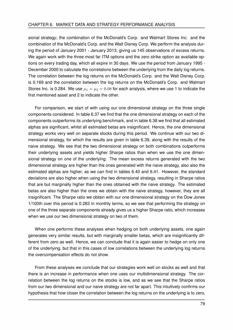
CHAPTER 6. MARKET DATA AND STRATEGY PERFORMANCE ANALYSIS
sional strategy; the combination of the McDonald’s Corp. and Walmart Stores Inc. and thecombination of the McDonald’s Corp. and the Walt Disney Corp. We perform the analysis dur-ing the period of January 2001 - January 2013, giving us 145 observations of excess returns.We again work with the three most far ITM options and the zero strike option as available op-tions on every trading day, which all expire in 30 days. We use the period from January 1995 -December 2000 to calculate the correlations between the underlying from the daily log returns.The correlation between the log returns on the McDonald’s Corp. and the Walt Disney Corp.is 0.169 and the correlation between the log returns on the McDonald’s Corp. and WalmartStores Inc. is 0.284. We use µ1 = µ2 = 0.08 for each analysis, where we use 1 to indicate thefirst mentioned asset and 2 to indicate the other.
For comparison, we start of with using our one dimensional strategy on the three singlecomponents considered. In table 6.37 we find that the one dimensional strategy on each of thecomponents outperforms its underlying benchmark, and in table 6.38 we find that all estimatedalphas are significant, whilst all estimated betas are insignificant. Hence, the one dimensionalstrategy works very well on separate stocks during this period. We continue with our two di-mensional strategy, for which the results are given in table 6.39, along with the results of thenaive strategy. We see that the two dimensional strategy on both combinations outperformstheir underlying assets and yields higher Sharpe ratios than when we use the one dimen-sional strategy on one of the underlying. The mean excess returns generated with the twodimensional strategy are higher than the ones generated with the naive strategy, also also theestimated alphas are higher, as we can find in tables 6.40 and 6.41. However, the standarddeviations are also higher when using the two dimensional strategy, resulting in Sharpe ratiosthat are but marginally higher than the ones obtained with the naive strategy. The estimatedbetas are also higher than the ones we obtain with the naive strategy, however, they are allinsignificant. The Sharpe ratio we obtain with our one dimensional strategy on the Dow Jones1/100th over this period is 0.283 in monthly terms, so we see that performing the strategy onone of the three separate components already gives us a higher Sharpe ratio, which increaseswhen we use our two dimensional strategy on two of them.
When one performs these analyses when hedging on both underlying assets, one againgenerates very similar results, but with marginally smaller betas, which are insignificantly dif-ferent from zero as well. Hence, we can conclude that it is again easier to hedge on only oneof the underlying, but that in this cases of low correlations between the underlying log returnsthe overcompensation effects do not show.
From these analyses we conclude that our strategies work well on stocks as well and thatthere is an increase in performance when one uses our multidimensional strategy. The cor-relation between the log returns on the stocks is low, and as we see that the Sharpe ratiosfrom our two dimensional and our naive strategy are not far apart. This intuitively confirms ourhypothesis that how closer the correlation between the log returns on the underlying is to zero,
79
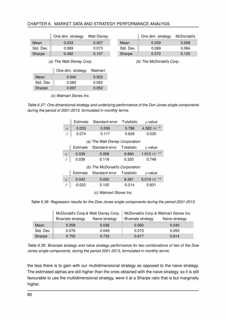
CHAPTER 6. MARKET DATA AND STRATEGY PERFORMANCE ANALYSIS
One dim. strategy Walt Disney
Mean 0.033 0.007Std. Dev. 0.069 0.073Sharpe 0.482 0.107
(a) The Walt Disney Corp.
One dim. strategy McDonald’s
Mean 0.039 0.008Std. Dev. 0.069 0.064Sharpe 0.572 0.120
(b) The McDonald’s Corp.
One dim. strategy Walmart
Mean 0.042 0.003Std. Dev. 0.060 0.052Sharpe 0.697 0.052
(c) Walmart Stores Inc.
Table 6.37: One dimensional strategy and underlying performance of the Don Jones single componentsduring the period of 2001-2013, formulated in monthly terms.
Estimate Standard error T-statistic p-value
α 0.033 0.006 5.786 4.382·10−8
β 0.074 0.117 0.629 0.530
(a) The Walt Disney CorporationEstimate Standard error T-statistic p-value
α 0.039 0.006 6.860 1.912·10−10
β 0.038 0.118 0.320 0.749
(b) The McDonald’s CorporationEstimate Standard error T-statistic p-value
α 0.042 0.005 8.361 5.019·10−14
β -0.022 0.102 -0.214 0.831
(c) Walmart Stores Inc.
Table 6.38: Regression results for the Dow Jones single components during the period 2001-2013.
McDonald’s Corp.& Walt Disney Corp. McDonald’s Corp & Walmart Stores Inc.Bivariate strategy Naive strategy Bivariate strategy Naive strategy
Mean 0.058 0.036 0.060 0.040Std. Dev. 0.076 0.049 0.073 0.050Sharpe 0.755 0.733 0.817 0.814
Table 6.39: Bivariate strategy and naive strategy performance for two combinations of two of the DowJones single components, during the period 2001-2013, formulated in monthly terms.
the less there is to gain with our multidimensional strategy as opposed to the naive strategy.The estimated alphas are still higher than the ones obtained with the naive strategy, so it is stillfavourable to use the multidimensional strategy, were it at a Sharpe ratio that is but marginallyhigher.
80

CHAPTER 6. MARKET DATA AND STRATEGY PERFORMANCE ANALYSIS
Estimate Standard error T-statistic p-value
α 0.058 0.006 9.076 8.136·10−16
β 0.110 0.130 0.845 0.400
(a) Bivariate strategy
Estimate Standard error T-statistic p-value
α 0.036 0.004 8.772 4.742·10−15
β 0.056 0.085 0.658 0.511
(b) Naive strategy
Table 6.40: Regression results of the bivariate strategy and naive strategy of the McDonald’s Corp.and Walt Disney Corp. with the market excess returns as explanatory variable, during the period of2001-2013.
Estimate Standard error T-statistic p-value
α 0.060 0.001 9.815 1.058·10−17
β 0.064 0.126 0.511 0.610
(a) Bivariate strategy
Estimate Standard error T-statistic p-value
α 0.040 0.004 9.734 1.708·10−17
β 0.008 0.085 0.092 0.927
(b) Naive strategy
Table 6.41: Regression results of the bivariate strategy and naive strategy of the McDonald’s Corp.and Walmart Stores Inc. with the market excess returns as explanatory variable, during the period of2001-2013.
Considering the analyses of our multidimensional strategy performance in all four periods,for indices and stocks, we conclude that our strategy performs very well. The generated Sharperatios are higher than those of the individual benchmarks and higher then the ones obtainedwith our one dimensional strategy on the individual benchmarks. The estimated alphas aresignificantly different from zero and all betas are insignificant, though, in times of high volatilitythey do tend to be high, but still insignificant. For underlying with high correlation one is betterof hedging on only one of the assets, as there are slight overcompensation effects when onehedges on both, though the results do not differ much. When correlation is low, then the hedgeworks marginally better when hedging on both assets. Hedging on only one of the underlyingmakes the strategy easier to implement and gives one almost the same results. We also findthat the multidimensional strategy outperforms our naive strategy and that the magnitude ofoutperformance increases when the correlation between the benchmarks increases.
81

CHAPTER 7
CONCLUSIONS AND RECOMMENDATIONS
FOR FURTHER RESEARCH
In this chapter we present the most important conclusions that we can draw from our researchand a few recommendations we can make for further research. We start with our conclusions:
• In a Black-Scholes world, one cannot generate a significant alpha with our tradingstrategies on options with discrete strikes, neither in the one dimensional case,nor in the multidimensional case.
Guasoni et al. [8] have already drawn this conclusion for the one dimensional case, usingoptions with continuous strikes. As we have seen in our simulations in chapter 5, also when us-ing European call options with discrete strikes, one cannot generate superior performance bytrading dynamically in options according to our strategies when one works in a Black-Scholesworld, where benchmark assets follow geometric Brownian motions with constant drift anddiffusion, and options are priced according to the Black-Scholes formula, neither when consid-ering one benchmark asset, nor when considering two.
• When using data obtained from the market, one can generate a statistically signif-icant alpha with our trading strategies. The results improve when one considersmore benchmark assets to invest on.
From the results of chapter 6 we can conclude that our strategy for the one dimensionalcase works very well, as the reported Sharpe ratios obtained with the strategy on each con-sidered benchmark asset are high and the generated alphas are significantly different fromzero at a 5% significance level. Even in times of high volatility on the underlying assets, thestrategy manages to outperform holding the benchmark asset. When one considers more thanone benchmark asset to trade options on and uses our multidimensional strategy, even betterresults are obtained. The obtained Sharpe ratios are generally higher than the ones obtainedin the one dimensional case and the alphas obtained are significant.
• Far in-the-money options and the zero strike option are favourable products in ourstrategies.
From our simulations and market data analyses we can conclude that our portfolio selec-tion each trading day places most weight on the most far in-the-money options and the zero
83
CHAPTER 7. CONCLUSIONS AND RECOMMENDATIONS FOR FURTHER RESEARCH
strike option, thus, the benchmark asset itself. When considering only the three most far in-the-money options in our dataset and this zero strike option as available options every tradingday, the results obtained even tend to be better than the ones obtained when considering allavailable options. This is the case for both the one dimensional strategy and the multidimen-sional strategy. Another positive side of this conclusion is that when a hedge fund managerwants to implement this strategy, he only has to consider a few products to invest on, insteadof a wide range. This makes the strategy easier to implement.
• Our way of hedging out the strategy’s sensitivity with respect to market excessreturns works, but tends to produce high regression betas in times of high volatilityon the market. When considering more than one benchmark asset in the strategyand when one uses all benchmarks to hedge out the sensitivity with respect tomarket excess returns, one can get overcompensated results that make the hedgeworse.
From our simulation results we can conclude that the beta-hedge works well when oneconsiders a Black-Scholes framework. The obtained betas are very close to zero and are sta-tistically insignificantly different from zero at a 5% significance level, for the one dimensionalstrategy, as well as for the multidimensional strategy. For the multidimensional strategy weencounter overcompensation effects when hedging on both underlying in the simulation, butwhen one hedges on only one of the underlying, the beta-hedge performs well. When one usesour one dimensional strategy with historical market data, the obtained betas are insignificantover every period we have analyzed, for every benchmark asset we have considered. Theobtained betas over the period 2007-2013, where volatilities are high, are larger than thoseover the period of 2003-2006, where volatilities are low. However, the betas obtained over1996/1998-2002, where volatility is high as well, do not differ much from those obtained over2003-2006. The credit crisis and global recession period contains a very large peak in volatilityfor all considered benchmark assets, which we think causes the high betas during that period.Also, with our multidimensional strategy we find similar results and we conclude that the effectof the high volatilities is even greater, though the obtained betas are still insignificant, so thehedge is still performs adequate. In the analyses with historical data we only find the overcom-pensation effects of hedging on both underlying when the correlation between the log returnsof the underlying is high, but on a marginal scale. The strategy is easier to implement whenone hedges only with respect to one underlying and the results are very similar in the caseswe have studied, so we recommend to omit the hedge on the second underlying.
• Our multidimensional strategy outperforms a naive strategy that spreads oneswealth and invests it on the considered benchmarks using our one dimensionalstrategy. The magnitude of this outperformance increases as the correlation be-tween the considered benchmarks increases.
When the correlation between the benchmarks would be zero, it would be optimal to splitones capital into equal parts and use each part to invest on a different benchmark using our
84
CHAPTER 7. CONCLUSIONS AND RECOMMENDATIONS FOR FURTHER RESEARCH
one dimensional strategy. As we have seen for the S&P 500 and the Russell 2000, for whichcorrelation is high, our two dimensional strategy outperforms this naive strategy, yielding ahigher Sharpe ratio and an insignificant beta, whereas the naive strategy produces a significantbeta. We have also investigated the differences between these strategies for two combinationsof three stocks in the Dow Jones index, for which the correlations are lower. We see that theSharpe ratios obtained with our multidimensional strategy are but marginally larger than thoseobtained with the naive strategy and for both strategies the generated betas are insignificant.
• When one hedges out the strategy’s sensitivity with respect to the market excessreturns using a position in the benchmark asset itself, but treating this benchmarkasset as if it were the market works better than more complicated approaches.Also, improving the model with a dynamic growth rate in the geometric Brownianmotion does not yield a significant improvement to the results.
As we have seen in our one dimensional data analysis, one does not win much by notchoosing βmkt of the underlying equal to something else than one. The results do not improve,and sometimes actually get worse by constructing this sensitivity parameter from historical dataand then using it as a constant, or updating it dynamically as one obtains more information onthe benchmarks and the market during the period on which we use our strategy. Making themodel more complicated, but more realistic, by making the growth rate in the geometric Brow-nian motion a function of time, does not bring any significant improvements to the results, soone can just treat this drift as a constant in the model.
We conclude this thesis with a few recommendations for further research, which in ouropinion interesting to pursue:
• Improve the stability of the covariance matrix of option excess returns.
The entries in the covariance matrix tend to get very, very small sometimes, leaving thecovariance matrix prone to numerical errors. This can cause the covariance matrix to becomenon positive semi definite, which cannot be the case for covariance matrices. We have encoun-tered this problems when using volatilities based on a historical period of 30 days, in stead of60, which we use in our analyses, and when using dynamic correlation coefficients in the mul-tidimensional case. We suspect that a dynamic correlation coefficient can improve the results.Thus far, we were not able to explain why the problem occurs exactly, so we recommend furtherresearch on this.
• Introduce trading costs and margins to the model.
We have worked with frictionless markets, as this is convenient for research. Our simpleapproach to introducing trading costs was too simple. To make the analysis more realistic, wesuggest to implement trading costs to the model. Also, we take quite substantial short positionsin some options in our portfolio. In practice, one has to make a down payment, a ‘margin’, to
85
CHAPTER 7. CONCLUSIONS AND RECOMMENDATIONS FOR FURTHER RESEARCH
be allowed to do this. We omit these margins, as there is not much data available on them.The effects on the results might be interesting, though.
• Extend the strategies to allow put options and American exercise style options.
A lot of traded options are of American exercise style and a lot of previous research sug-gests out-of-the-money puts to be favourable products. One can see our position in far in-the-money calls as positions in out-of-the-money puts, in the underlying, and in cash by the put-callparity, but introducing the actual product might provide interesting results. The problem withAmerican put options is the fact one can exercise them before the expiry date, so the strategyhas to be adapted to account for this.
• Test the strategies with actual traded options.
For convenience, we have worked with interpolated options throughout this research, whichare not actually traded on the market, but are based on options that are. We suggest toextend the strategies in such a way that one can work with actual traded options, on which theOptionmetrics database also contains a lot of data. The problem with the traded options is thatthe options do not all have the same time to expiration and that in practice it can happen thaton a certain trading day there are options available on one benchmark, but not on the other.As our strategy assumes that all options always expire at the same date and are traded at thesame date, it needs some extensions to account for actual traded options.
• Implement a stochastic volatility model with jump components.
We have seen in our market data analysis that very sudden, large movements in the un-derlying can lead to substantial excess returns (positive and negative) on our portfolio choice,as we ‘bet’ on a certain scenario, but end up in a completely different one. These large move-ments can be caused by market crashes etc. A model that can account for sudden jumps in theprice process and the volatility process might reduce the magnitude of these negative returns,but might also decrease the magnitude of our strong positive results. We think the effects ofthis implementation could be very interesting, but the explicit expressions for the expected op-tion excess returns and covariances between them might be much harder to obtain. Broadieet al. [2] and Eraker [3], for example, study these kind of models for their trading strategies.
86

Bibliography
[1] J. D. Coval and T. Shumway, “Expected option returns,” The Journal of Finance, vol. 56,pp. 983–1009, June 2001.
[2] M. Broadie, M. Chernov, and M. Johannes, “Understanding index option returns,” TheReview of Financial Studies, vol. 22, pp. 4493–4529, May 2009.
[3] B. Eraker, “The performance of model based option trading strategies,” Review of Deriva-tives Research, vol. 16, pp. 1–23, April 2013.
[4] C. S. Jones, “A nonlinear factor analysis of s&p 500 index option returns,” The Journal ofFinance, vol. LXI, pp. 2325–2363, October 2006.
[5] N. Kapadia and E. Szado, “The risk and return characteristics of the buy write strategy onthe russel 2000 index,” Journal of Alternative Investments, vol. 9, pp. 39–56, Spring 2007.
[6] J. Liang, S. Zhang, and D. Li, “Optioned portfolio selection: Models and analysis,” Mathe-matical Finance, vol. 18, pp. 569–593, October 2008.
[7] P. Santa-Clara and A. Saretto, “Option strategies: Good deals and margin calls,” Journalof Financial Markets, vol. 12, pp. 391–417, January 2009.
[8] P. Guasoni, G. Huberman, and Z. Wang, “Performance maximization of actively managedfunds,” Journal of Financial Economics, vol. 101, pp. 574–595, September 2011.
[9] H. Markowitz, “Portfolio selection,” The Journal of Finance, vol. 7, pp. 77–91, March 1952.
[10] J. H. Cochrane, Asset Pricing. 3 Market Place, Woodstock, Oxfordshire: Priceton Univer-sity Press, 2001.
I


APPENDIX A
PROOFS
A.1 Proof of Theorem 3.2.3
Since the only unknown in equation (3.10) is EP [(ST −Ki)+], we will focus on this term and
use that the underlying price process is a geometric Brownian motion. Since the ε in equation(3.3) is standard normal distributed under the physical measure, we have:
EP [(ST −Ki)+] =
∫(ST −Ki)
+N ′(x) dx =
∫ (St · e
(µ−σ
2
2
)∆t+σ
√∆tx −Ki
)+
N ′(x) dx,
for which the integrand is only nonzero if
St · e(µ−σ
2
2
)∆t+σ
√∆tx −Ki > 0
e
(µ−σ
2
2
)∆t+σ
√∆tx
> Ki/St(µ− σ2
2
)∆t+ σ
√∆tx > ln [Ki/St]
x >ln [Ki/St]−
(µ− σ2
2
)∆t
σ√
∆t= d1,
so, we have
EP [(ST −Ki)+] =
∫ (St · e
(µ−σ
2
2
)∆t+σ
√∆tx −Ki
)+
N ′(x) dx
=
∫ ∞d1
(St · e
(µ−σ
2
2
)∆t+σ
√∆tx −Ki
)N ′(x) dx
=
∫ ∞d1
St · e(µ−σ
2
2
)∆t+σ
√∆tx
N ′(x) dx−∫ ∞d1
KiN′(x) dx
= St · e(µ−σ
2
2
)∆t∫ ∞d1
eσ√
∆txN ′(x) dx−KiN(−d1),
where for the last integral we use that the normal distribution is symmetric. To find an explicitexpression for the first integral, we will write the exponential times the PDF as a standard-ized normal PDF with mean µ∗ and standard deviation σ∗, by completing the square in theexponential:
− (x− µ∗)2
2σ∗2=−1
2σ∗2
[x2 − 2µ∗x+ µ∗
2]
= σ√
∆tx− 1
2x2 + C
⇒ σ∗ = 1, µ∗ = σ√
∆t, and C = −σ2
2∆t.
III

APPENDIX A. PROOFS
Since we do not have C in our initial exponential, we have to compensate for this term bymultiplication with e−C , and since we are now using a standardized normal distribution, wemust subtract µ∗ from our lower integration bound, yielding:
EP [(ST −Ki)+] = St · e
(µ−σ
2
2
)∆t∫ ∞d1
eσ√
∆txN ′(x) dx−KiN(−d1)
= St · e(µ−σ
2
2
)∆teσ2
2∆t
∫ ∞d1−µ∗
1√2πe−
(x−µ∗)22 dx−KiN(−d1)
= St · eµ∆t
∫ ∞d2
N ′(x) dx−KiN(−d1)
= St · eµ∆tN(−d2)−KiN(−d1)
= St · eµ∆tN(d2)−KiN(d1),
where
d1 = −d1 = −ln [Ki/St]−
(µ− σ2
2
)∆t
σ√
∆t=
ln [St/Ki] +(µ− σ2
2
)∆t
σ√
∆t,
d2 = −d2 = −(d1 − σ√
∆t) = d1 + σ√
∆t =ln [St/Ki] +
(µ+ σ2
2
)∆t
σ√
∆t.
Plugging this expression in to equation (3.10) yields the result.
A.2 Proof of Theorem 3.2.4
We first rewrite cov(ropti , roptj
)in terms of expectations:
cov(ropti , roptj
)= cov
(e−rf∆t(ST −Ki)
+
Ci− 1,
e−rf∆t(ST −Kj)+
Cj− 1
)= cov
(e−rf∆t(ST −Ki)
+
Ci,e−rf∆t(ST −Kj)
+
Cj
)= EP
[e−rf∆t(ST −Ki)
+
Ci· e−rf∆t(ST −Kj)
+
Cj
]− EP
[e−rf∆t(ST −Ki)
+
Ci
]EP[e−rf∆t(ST −Kj)
+
Cj
]=e−2rf∆t
CiCjEP [(ST −Ki)
+(ST −Kj)+]− (mi + 1)(mj + 1),
in which the only unknown term is EP [(ST −Ki)+(ST −Kj)
+]. We obtain this term throughintegration, in a similar fashion as with the proof of Theorem 3.2.3:
EP [(ST −Ki)+(ST −Kj)
+]
=
∫(ST −Ki)
+(ST −Kj)+N ′(x) dx
IV

APPENDIX A. PROOFS
=
∫ (St · e(µ−σ
2
2)∆t+σ
√∆tx −Ki
)+(St · e(µ−σ
2
2)∆t+σ
√∆tx −Kj
)+
N ′(x) dx
=
∫ ∞d5
(St · e(µ−σ
2
2)∆t+σ
√∆tx −Ki
)(St · e(µ−σ
2
2)∆t+σ
√∆tx −Kj
)N ′(x) dx
= S2t e
(2µ−σ2)∆t
∫ ∞d5
e2σ√
∆txN ′(x) dx− St(Ki +Kj)e
(µ−σ
2
2
)∆t∫ ∞d5
eσ√
∆txN ′(x) dx
+KiKj
∫ ∞d5
N ′(x) dx,
in which we again complete the square in the first two integrals, subtract the corresponding µ∗
from the lower integration bound and compensate for the corresponding eC-terms that are notin our initial integrals. This yields:
= S2t e
(2µ+σ2)∆tN(−d3)− St(Ki +Kj)eµ∆tN(−d4) +KiKjN(−d5)
= S2t e
(2µ+σ2)∆tN(d3)− St(Ki +Kj)eµ∆tN(d4) +KiKjN(d5),
where
d5 =ln[max(Ki,Kj)/St]−
(µ−σ
2
2
)∆t
σ√
∆t, d5 = −d5 =
ln[St/max(Ki,Kj)]+(µ−σ
2
2
)∆t
σ√
∆t,
d4 = d5 − σ√
∆t, d4 = −d4 =ln[St/max(Ki,Kj)]+
(µ+σ2
2
)∆t
σ√
∆t,
d3 = d5 − 2σ√
∆t, d3 = −d3 =ln[St/max(Ki,Kj)]+
(µ+ 3σ2
2
)∆t
σ√
∆t.
Plugging this expectation into the equation for the covariance we derived at the start of thisproof gives us the result.
A.3 Proof of Theorem 4.1.1
We write out the derivation for covariances of type 1 to full extent. The other two are specialcases of this case.
For i = 1, . . . , n1 − 1 and j = 1, . . . , n2 − 1 we have
cov(r(1)i , r
(2)j ) = cov
(e−rf∆t(S
(1)T −K
(1)i )+
C(1)i
− 1,e−rf∆t(S
(2)T −K
(2)j )+
C(2)j
− 1
)
= cov
(e−rf∆t(S
(1)T −K
(1)i )+
C(1)i
,e−rf∆t(S
(2)T −K
(2)j )+
C(2)j
)
=e−2rf∆t
C(1)i C
(2)j
EP[(S
(1)T −K
(1)i )+(S
(2)T −K
(2)j )+
]
− EP
[e−rf∆t(S
(1)T −K
(1)i )+
C(1)i
]EP
[e−rf∆t(S
(2)T −K
(2)j )+
C(2)j
]
=e−2rf∆t
C(1)i C
(2)j
EP[(S
(1)T −K
(1)i )+(S
(2)T −K
(2)j )+
]− (m
(1)i + 1)(m
(2)j + 1),
V

APPENDIX A. PROOFS
in which we see that again the only unknown term in the equation, is the expectation. Wederive this term with the same methodology as in the single underlying case.
EP[(S
(1)T −K
(1)i )+(S
(2)T −K
(2)j )+
]=
∫∫(S
(1)t e(µ1−
σ212
)∆t+σ1√
∆tx1 −K(1)i )+(S
(2)t e(µ2−
σ222
)∆t+σ2√
∆tx2 −K(2)j )+ ·MN ′(x1, x2) dx1 dx2
=
∫ ∞d21
∫ ∞d11
(S(1)t e(µ1−
σ212
)∆t+σ1√
∆tx1 −K(1)i )(S
(2)t e(µ2−
σ222
)∆t+σ2√
∆tx2 −K(2)j ) ·MN ′(x1, x2) dx1 dx2,
where MN ′(x1, x2) is the PDF of the standard bivariate normal distribution, and
d11 =
ln[K
(1)i /S
(1)t
]−(µ1 −
σ212
)∆t
σ1
√∆t
, d21 =
ln[K
(2)j /S
(2)t
]−(µ2 −
σ222
)∆t
σ2
√∆t
.
We continue the derivation:
= S(1)t S
(2)t e(µ1−
σ212
+µ2−σ222
)∆t
∫ ∞d21
∫ ∞d11
e(σ1x1+σ2x2)√
∆tMN ′(x1, x2) dx1 dx2
−K(1)i S
(2)t e(µ2−
σ222
)∆t
∫ ∞d21
∫ ∞d11
eσ2x2√
∆tMN ′(x1, x2) dx1 dx2
−K(2)j S
(1)t e(µ1−
σ212
)∆t
∫ ∞d21
∫ ∞d11
eσ1x1√
∆tMN ′(x1, x2) dx1 dx2
+K(1)i K
(2)j
∫ ∞d21
∫ ∞d11
MN ′(x1, x2) dx1 dx2.
For each integrand we again complete the square to make it a standardized bivariate normalPDF. Just as in the one dimensional case, we assume that σ∗1 = σ∗2 = 1. The covariance matrixof MN ′(x1, x2) is given by
Σ =
[1 ρ12
ρ12 1
],
thus, when we write out the exponentials of each integrand plus a constant for which we haveto compensate and set it equal to the exponential of the standardized bivariate normal PDF,we get the general equation (which holds for higher dimensions of N as well):
C + α′x− 1
2x′Σ−1x = −1
2(x− µ∗)′Σ−1(x− µ∗)
C + α′x− 1
2x′Σ−1x = −1
2x′Σ−1x+ x′Σ−1µ∗ − 1
2µ∗′Σ−1µ∗,
in which all vectors are two dimensional column vectors. The vector α is composed of theelements in the first exponential of each integrand that are multiplicated with the elementsof the vector x = x1, x2′. For example, for our first integral we find α = σ1
√∆t, σ2
√∆t′,
making the term e(σ1x1+σ2x2)∆t, for the second we find α = 0, σ2
√∆t′ and for the third we find
α = σ1
√∆t, 0′. The fourth does not need an alteration. From these equations we deduce
⇒ C = −1
2µ∗′Σ−1µ∗, α′x = x′Σ−1µ∗,
⇒ µ∗ = Σα.
VI

APPENDIX A. PROOFS
So now we have for each integral the constant exponential for which we have to compensateand the shift µ∗ in the lower boundaries of the double integrals. The integrands can now allbe expressed as standardized bivariate normal PDFs, so we can express the double integralsin terms of the CDF of the standard bivariate normal distribution, with entries derived from theshifted lower boundaries as we did in the single underlying case. Combining the terms resultsin the first claim of the theorem and its values for d1, d2, . . . , d8, which arise from the shifted d1
1
and d21 terms for each integral. In higher dimensions of underlying, one will get the same sort
of expressions, but since α and Σ are of higher dimension, one will get more correlation termsin the constant for which we have to compensate and more standard deviation terms in ourµ∗-expressions. The same formulas can be used for every Sij .
Now, for covariances of the second kind, one follows the same derivation, but the last twointegrals disappear, because one has a strike equal to zero. Also, because of one strike iszero, only one of the double integrals has a lower boundary, the other one (integrating over theunderlying which has strike zero) will have a lower boundary of −∞ and will thus integrate thebivariate normal density to a normal density, hence, one gets the result in terms of the normalCDF, as made in our second claim.
The covariances of the third kind are both on options with strike zero, hence, all integralswith terms of K before them will disappear and all lower boundaries will remain −∞, hence,after standardizing these integrands, one remains with a double integral over a probabilitydensity over the entire real axis, which yields one. Therefore, only the terms before the integralremain, and one arrives at the final claim.
VII


APPENDIX B
TABLES
In this appendix we present the tables with results from our data analysis in chapter 6 whichwe did not present in the chapter itself. The tables present analyses of the performance ofholding individual options for all underlying and periods considered, expected excess returnson these options and the mean absolute weights of these options in the portfolios in the oneand two dimensional case.
B.1 Mean absolute portfolio weights
Option ∆ S&P 500 NASDAQ 100 Russell 2000 DowJones 1/100th
0.20 0.020 0.017 0.021 0.0270.25 0.051 0.039 0.040 0.0690.30 0.054 0.038 0.030 0.0520.35 0.070 0.041 0.032 0.0400.40 0.077 0.050 0.043 0.0440.45 0.078 0.058 0.047 0.0480.50 0.82 0.062 0.054 0.0500.55 0.94 0.070 0.065 0.0590.60 0.087 0.076 0.064 0.0530.65 0.097 0.074 0.063 0.0660.70 0.156 0.173 0.129 0.1420.75 0.500 0.557 0.490 0.5340.80 0.950 0.971 1.204 0.9341 8.758 5.999 10.251 8.510
Table B.1: Mean absolute portfolio weights for all underlying during the period 1996/1998-2013, usingthe one dimensional strategy
IX
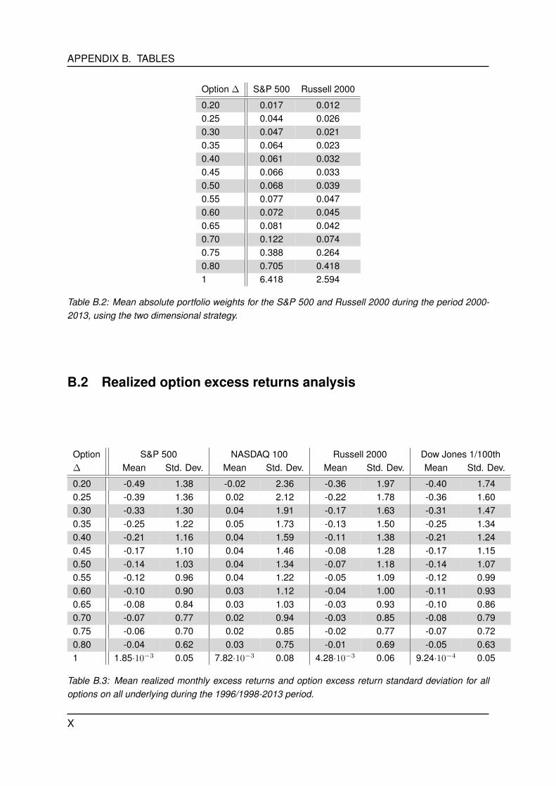
APPENDIX B. TABLES
Option ∆ S&P 500 Russell 2000
0.20 0.017 0.0120.25 0.044 0.0260.30 0.047 0.0210.35 0.064 0.0230.40 0.061 0.0320.45 0.066 0.0330.50 0.068 0.0390.55 0.077 0.0470.60 0.072 0.0450.65 0.081 0.0420.70 0.122 0.0740.75 0.388 0.2640.80 0.705 0.4181 6.418 2.594
Table B.2: Mean absolute portfolio weights for the S&P 500 and Russell 2000 during the period 2000-2013, using the two dimensional strategy.
B.2 Realized option excess returns analysis
Option S&P 500 NASDAQ 100 Russell 2000 Dow Jones 1/100th∆ Mean Std. Dev. Mean Std. Dev. Mean Std. Dev. Mean Std. Dev.
0.20 -0.49 1.38 -0.02 2.36 -0.36 1.97 -0.40 1.740.25 -0.39 1.36 0.02 2.12 -0.22 1.78 -0.36 1.600.30 -0.33 1.30 0.04 1.91 -0.17 1.63 -0.31 1.470.35 -0.25 1.22 0.05 1.73 -0.13 1.50 -0.25 1.340.40 -0.21 1.16 0.04 1.59 -0.11 1.38 -0.21 1.240.45 -0.17 1.10 0.04 1.46 -0.08 1.28 -0.17 1.150.50 -0.14 1.03 0.04 1.34 -0.07 1.18 -0.14 1.070.55 -0.12 0.96 0.04 1.22 -0.05 1.09 -0.12 0.990.60 -0.10 0.90 0.03 1.12 -0.04 1.00 -0.11 0.930.65 -0.08 0.84 0.03 1.03 -0.03 0.93 -0.10 0.860.70 -0.07 0.77 0.02 0.94 -0.03 0.85 -0.08 0.790.75 -0.06 0.70 0.02 0.85 -0.02 0.77 -0.07 0.720.80 -0.04 0.62 0.03 0.75 -0.01 0.69 -0.05 0.631 1.85·10−3 0.05 7.82·10−3 0.08 4.28·10−3 0.06 9.24·10−4 0.05
Table B.3: Mean realized monthly excess returns and option excess return standard deviation for alloptions on all underlying during the 1996/1998-2013 period.
X
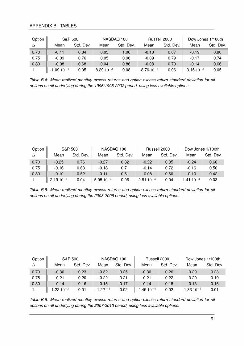
APPENDIX B. TABLES
Option S&P 500 NASDAQ 100 Russell 2000 Dow Jones 1/100th∆ Mean Std. Dev. Mean Std. Dev. Mean Std. Dev. Mean Std. Dev.
0.70 -0.11 0.84 0.05 1.06 -0.10 0.87 -0.19 0.800.75 -0.09 0.76 0.05 0.96 -0.09 0.79 -0.17 0.740.80 -0.08 0.68 0.04 0.86 -0.08 0.70 -0.14 0.661 -1.09·10−4 0.05 8.29·10−3 0.08 -8.76·10−4 0.06 -3.15·10−3 0.05
Table B.4: Mean realized monthly excess returns and option excess return standard deviation for alloptions on all underlying during the 1996/1998-2002 period, using less available options.
Option S&P 500 NASDAQ 100 Russell 2000 Dow Jones 1/100th∆ Mean Std. Dev. Mean Std. Dev. Mean Std. Dev. Mean Std. Dev.
0.70 -0.25 0.76 -0.27 0.82 -0.22 0.85 -0.24 0.600.75 -0.16 0.63 -0.18 0.71 -0.14 0.72 -0.16 0.500.80 -0.10 0.52 -0.11 0.61 -0.08 0.60 -0.10 0.421 2.19·10−3 0.04 5.05·10−3 0.06 2.81·10−3 0.04 1.41·10−3 0.03
Table B.5: Mean realized monthly excess returns and option excess return standard deviation for alloptions on all underlying during the 2003-2006 period, using less available options.
Option S&P 500 NASDAQ 100 Russell 2000 Dow Jones 1/100th∆ Mean Std. Dev. Mean Std. Dev. Mean Std. Dev. Mean Std. Dev.
0.70 -0.30 0.23 -0.32 0.25 -0.30 0.26 -0.29 0.230.75 -0.21 0.20 -0.22 0.21 -0.21 0.22 -0.20 0.190.80 -0.14 0.16 -0.15 0.17 -0.14 0.18 -0.13 0.161 -1.22·10−3 0.01 -1.22·−3 0.02 -4.45·10−4 0.02 -1.33·10−3 0.01
Table B.6: Mean realized monthly excess returns and option excess return standard deviation for alloptions on all underlying during the 2007-2013 period, using less available options.
XI
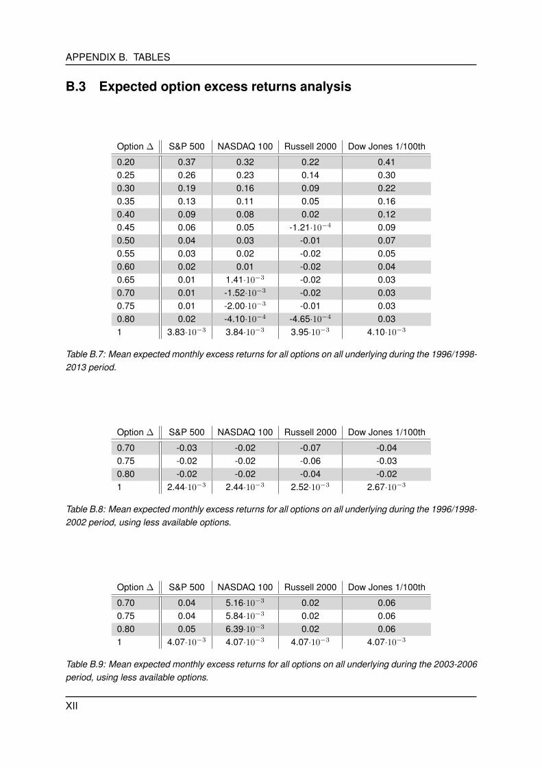
APPENDIX B. TABLES
B.3 Expected option excess returns analysis
Option ∆ S&P 500 NASDAQ 100 Russell 2000 Dow Jones 1/100th
0.20 0.37 0.32 0.22 0.410.25 0.26 0.23 0.14 0.300.30 0.19 0.16 0.09 0.220.35 0.13 0.11 0.05 0.160.40 0.09 0.08 0.02 0.120.45 0.06 0.05 -1.21·10−4 0.090.50 0.04 0.03 -0.01 0.070.55 0.03 0.02 -0.02 0.050.60 0.02 0.01 -0.02 0.040.65 0.01 1.41·10−3 -0.02 0.030.70 0.01 -1.52·10−3 -0.02 0.030.75 0.01 -2.00·10−3 -0.01 0.030.80 0.02 -4.10·10−4 -4.65·10−4 0.031 3.83·10−3 3.84·10−3 3.95·10−3 4.10·10−3
Table B.7: Mean expected monthly excess returns for all options on all underlying during the 1996/1998-2013 period.
Option ∆ S&P 500 NASDAQ 100 Russell 2000 Dow Jones 1/100th
0.70 -0.03 -0.02 -0.07 -0.040.75 -0.02 -0.02 -0.06 -0.030.80 -0.02 -0.02 -0.04 -0.021 2.44·10−3 2.44·10−3 2.52·10−3 2.67·10−3
Table B.8: Mean expected monthly excess returns for all options on all underlying during the 1996/1998-2002 period, using less available options.
Option ∆ S&P 500 NASDAQ 100 Russell 2000 Dow Jones 1/100th
0.70 0.04 5.16·10−3 0.02 0.060.75 0.04 5.84·10−3 0.02 0.060.80 0.05 6.39·10−3 0.02 0.061 4.07·10−3 4.07·10−3 4.07·10−3 4.07·10−3
Table B.9: Mean expected monthly excess returns for all options on all underlying during the 2003-2006period, using less available options.
XII

APPENDIX B. TABLES
Option ∆ S&P 500 NASDAQ 100 Russell 2000 Dow Jones 1/100th
0.70 0.04 0.02 0.02 0.060.75 0.04 0.01 0.02 0.060.80 0.04 0.02 0.02 0.061 5.33·10−3 5.33·10−3 5.33·10−3 5.33·10−3
Table B.10: Mean expected monthly excess returns for all options on all underlying during the 2007-2013 period, using less available options.
XIII

APPENDIX B. TABLES
XIV