Constant scalar curvature

Kahler metrics on fibred

complex surfaces

Joel Fine

Imperial College

1

Why look for cscK metrics?

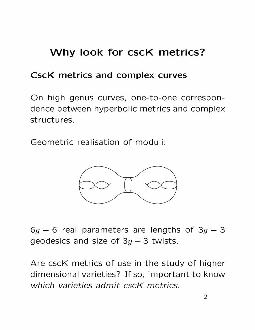
CscK metrics and complex curves

On high genus curves, one-to-one correspon-

dence between hyperbolic metrics and complex

structures.

Geometric realisation of moduli:

6g − 6 real parameters are lengths of 3g − 3

geodesics and size of 3g − 3 twists.

Are cscK metrics of use in the study of higher

dimensional varieties? If so, important to know

which varieties admit cscK metrics.2

Kahler-Einstein metrics

The Ricci form ρ of a Kahler metric is deter-mined by curvature of the canonical bundle:ρ = −iFK.

A Kahler-Einstein metric is proportional to itsRicci form: λω = ρ, for some constant λ.

Since [ρ] = 2πc1, necessary condition is that c1is zero or definite.

Taking traces: KE ⇒ cscK.

CscK and λ[ω] = 2πc1 ⇒ KE. This followsfrom Kahler identities and Hodge theory:

• [Λ, ∂] = i∂∗, so cscK ⇒ ρ harmonic;

• λ[ω] = [ρ] ⇒ λω = ρ.

CscK is generalisation of KE.

3

Lots of work has been done on finding and

using KE metrics.

• c1 < 0 (Aubin) and c1 = 0 (Yau) ⇒ KE.

• c1 > 0 much less is known. Certainly some

are not KE. For a Fano surface X, X is KE

⇔ Aut(X) is reductive (Tian). In higher

dims this is necessary, but not sufficient

condition for KE.

• Existence of KE metrics give results in al-

gebraic geometry e.g. Chern number in-

equalities, rigidity of P2; use of CYs in Mir-

ror symmetry.

4

Stably polarised varieties

Want to form a moduli space of polarised vari-eties e.g. consider all subvarieties of Pn moduloaction of GL(n + 1, C).

Want more than taxonomy; want geometricstructure on moduli space.

Need to exclude unstable orbits. Moduli ofstably polarised varieties has good geometry(GIT).

Leaves vital question: when is a given varietystable?

5

Conjecture. For (X, L) a smooth polarised va-

riety, (X, L) is K-stable if and only if −2πc1(L)

contains cscK metric.

Due to Yau in KE case, Tian in cscK case,

Donaldson in symplectic case.

Remarkable: relates two deep problems, one

entirely algebraic, the other analytic.

Fits into well studied framework: symplectic

reduction vs GIT (Donaldson). Cf. Hitchin–

Kobayashi correspondence.

Addresses question of which projective vari-

eties and which ample classes admit cscK met-

rics.

Known that cscK ⇒ K-stable (Chen–Tian).

Converse not yet proved.

6

K-stability not easy to check for. New concept

of slope-stability of (X, L) has been suggested

which is easier to use. (Again cf. holomorphic

bundles.)

K-stable ⇒ SS (Ross-Thomas). Not known

whether SS ⇒ K-stable.

There exist X with some (X, L) cscK, other

(X, L) not slope stable, hence not cscK (e.g.

P2 blown up four times.)

Summary

If DTY is correct, should be able to study sta-

bly polarised varieties via cscK metrics. This

should be the correct generalisation of situa-

tion for curves mentioned above.

One drawback is that hardly any examples of

cscK metrics are known outside of KE case.7

The constant scalar curvature equation

Parametrise Kahler forms in given class by open

set of functions (Kahler potentials):

ωφ = ω + i∂∂φ.

Attempt to solve Scal(ωφ) = const.

This is a fourth order fully non-linear PDE for

φ. Very hard to solve in general.

Geometric input is essential to find a solution

(knew this already from DTY).

8

If L denotes the linearisation of

φ 7→ Scal(ωφ),

then

L(φ) = D∗D(φ) +∇Scal ·∇φ

where D is defined by

D = ∂ ∇ : C∞ → Ω0,1(T )

and D∗ is L2 adjoint of D.

Leading order term of L is ∆2. So L is ellip-

tic. Can use standard theory of elliptic partial

differential equations.

9

CscK metrics on fibred complex

surfaces

math.DG/0401275

X compact connected complex surface.

π : X → Σ

a holomorphic submersion to a curve. Fibres

have high genus (≥2).

If g(Σ) = 0,1 easy to show X is quotient of

product S × Σ by group of isometries, hence

cscK. So assume high genus base.

V → X vertical tangent bundle. For any r let

κr = −2π (c1(V ) + rc1(Σ))

For large r these classes are ample.

10

Theorem. For all large r, κr contains a con-

stant scalar curvature Kahler metric.

Outline of proof:

1. Find explicit metrics ωr ∈ κr with

Scal(ωr) → const.

as r →∞.

2. Show that, for all large r, ωr can be per-

turbed to a genuinely cscK metric. Do this

by applying inverse function theorem to the

map

φ 7→ Scal(ωr + i∂∂φ).

Parameter dependence makes things awk-

ward.

11

Theorem (Quantitative IFT).

• Let F : B1 → B2 be a C1 map of Banach

spaces. Suppose that DF is an isomor-

phism with bounded inverse P .

• Let δ′ be radius of ball about 0 ∈ B1 on

which F − DF is Lipschitz with constant

(2‖P‖)−1.

• Let δ = δ′(2‖P‖)−1.

Then for any y ∈ B2 with

‖y − F (0)‖ < δ

there exists x ∈ B1 with F (x) = y. x is unique

solution with ‖x‖ < δ′.

12

Assume that ωr has been found with Scal(ωr) →const. Apply inverse function theorem to the

map

Sr : φ 7→ Scal(ωr + i∂∂φ)

The map depends on r, so δ depends on r

Need ‖Sr(0)− const.‖ ≤ δr to apply inverse

function theorem and prove the theorem.

Assuming linearisation is an isomorphism, there

are two key steps to perturbing to cscK metric:

• Need Scal(ωr) → const. very quickly.

• Need to control ‖Pr‖.

13

Derivative is an isomorphism

Recall that

Lφ = D∗D(φ) +∇Scal ·∇φ

Assume Scal(ωr) is nearly constant;

L(ωr) ≈ D∗D .

ker D∗D = ker D is functions with holomorphic

gradient.

No holomorphic vector fields on X; ker D = R.

D∗D has index zero, hence is an isomorphism

between spaces of functions with mean value

zero.

This implies same is true for L. So can apply

the inverse function theorem.

14

First order approximate solution

Hyperbolic metrics in fibres give metric in V .

Let ω0 = −iFV . Fibrewise restriction of ω0 is

hyperbolic metric on that fibre.

For large enough r,

ωr = ω0 + rωΣ

is Kahler; ωr ∈ κr.

r → ∞ is “stretching the base.” An example

of an adiabatic limit.

Scal(ωr) = −1 + O(r−1).

Adiabatic principle: in an adiabatic limit, the

local geometry is dominated by that of the fi-

bre.

Justified by the fact that locally (over the base)

the metric converges to the product S × C.

15

Second order approximate solution

Aim to find φ with

Scal(ωr + r−1i∂∂φ) = const. + O(r−2)

To O(r−2),

Scal(ωr + r−1i∂∂φ) = Scal(ωr) + r−1L(ωr)φ.

L(ωr) = LF + O(r−1)

LF surjective onto functions with mean valuezero over each fibre. Have decomposition

C∞(X) = C∞0 (X)⊕ C∞(Σ).

Can only remove C∞0 component of r−1 errorby adding r−1φ.

Setting C∞(Σ) component equal to constantgives non-linear PDE for ωΣ similar to cscKequation for base. Solution exists.

Now solve linear PDE, LFφ = Θ to remove C∞0component.

16

Higher order approximate solutions

Aim to find φ1, . . . , φn such that

Scal(ωr + i∂∂

∑r−jφj

)is O(r−n−1) from constant.

Find the φj recursively. Each is found by solv-

ing two linear PDEs, namely the linearisations

of the two non-linear PDEs mentioned above

(cscK metrics on the fibre, similar PDE on the

base).

Fredholm alternative for index zero operators:

the solutions to the non-linear problems are

“rigid,” so their linearisations are surjective.

Upshot is that, for each k, there exists an ap-

proximate solution with scalar curvature con-

verging to constant quicker than r−k.

17

Local analysis

Need to prove various local analytic estimates

(Sobolev inequalities, elliptic estimates etc.)

hold uniformly in r.

As r → ∞, Kahler structure near a fibre con-

verges to a product S × C.

Any estimate which holds over S×C holds uni-

formly over (X, ωr).

Analogous to study of tubes Y ×R which occurs

in Floer theory.

Key point is that the geometry of S × C is

uniformly bounded.

18

Global analysis

Upper bound on ‖Pr‖ is global result, so local

model not sufficient.

For global model, take Riemannian submersion

with hyperbolic metrics on fibres, rωΣ trans-

verse to fibres. Note that this is not Kahler.

Much easier to calculate the r dependence,

however.

Upper bound on ‖Pr‖ is essentially the same as

lower bound for first non-zero eigenvalue λ1(r)

of D∗D. Cf. finite dimensional linear algebra.

Need λ1(r) ≥ Cr−k for some k

19

Use fact that if for all φ with mean value zero,

‖Dφ‖2 ≥ c‖φ‖2

then λ1 ≥ c. (Norms are L2; everything is with

respect to metric ωr.) Again, cf. finite dimen-

sions.

Work with global model. Have explicit formu-

lae for r dependence of every term appearing

in above inequality. Gives bound

λ1(r) ≥ Cr−3.

I suspect best bound is λ1(r) ≥ Cr−2 (certainly

is in the case of a product). Not relevant to

the proof of the result, however.

20