Conformation tensor (1)

UCM, Oldroyd-B model:

λ5τ +τ = 2ηD

where5τ= τ −L · τ − τ ·LT

which we derived from the Lodge rubber like liquid with a single relaxation time:

τ (t) =∫ t

−∞

G

λe−(t−t′)/λ[Bt′(t)− I] dt′

η = Gλ.

Conformation tensor (2)

This can be written as:τ (t) = G

(c(t)− I)

with the conformation tensor c:

c(t) =1λ

∫ t

−∞e−(t−t′)/λBt′(t) dt′

Note: c = I in equilibrium (no deformation).

Comparing with the neo-Hookean elastic model:

τ = G(B − I)

we can interpret c as a “remaining elastic Finger strain”.

Conformation tensor (3)

The Oldroyd-B model written with c:

λ5c +c = I, τ = G

(c− I)

The Oldroyd-B model can also be derived from a stochastic microscopic theorywhere polymers are represented by linear springs. Here:

c ∼ 〈 ~Q~Q〉

with ~Q the end-to-end vector of a spring.

Important property of c:

c is a positive definite tensor

Conformation tensor (4)

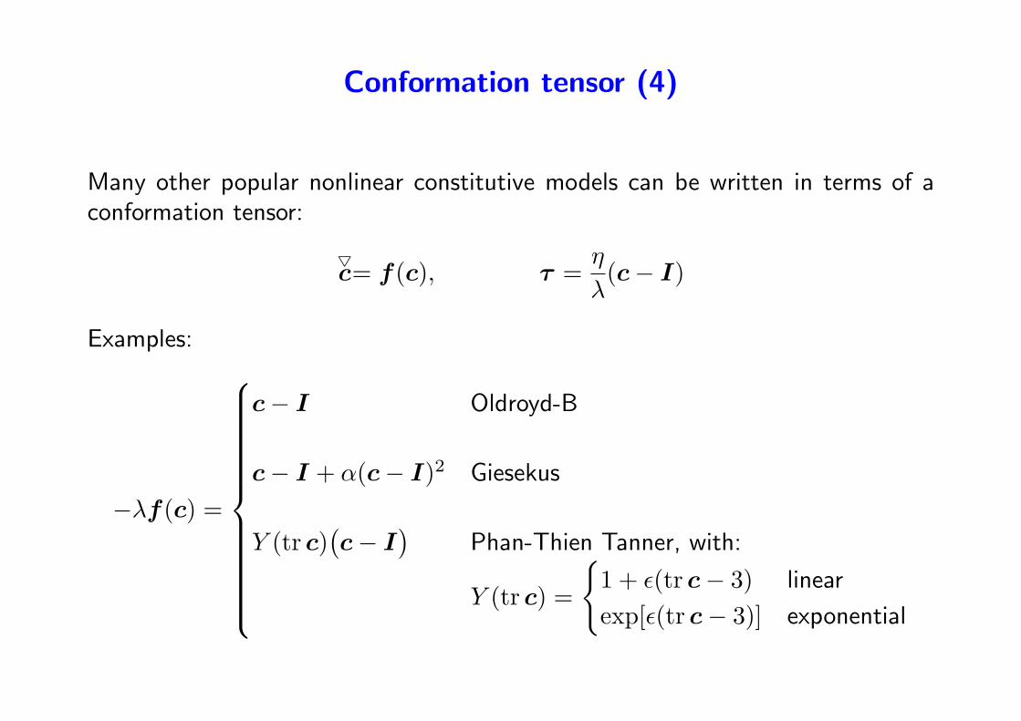
Many other popular nonlinear constitutive models can be written in terms of aconformation tensor:

5c= f(c), τ =

η

λ(c− I)

Examples:

−λf(c) =

c− I Oldroyd-B

c− I + α(c− I)2 Giesekus

Y (tr c)(c− I) Phan-Thien Tanner, with:

Y (tr c) =

1 + ε(tr c− 3) linear

exp[ε(tr c− 3)] exponential

Rheometric functions (1)

σ11

σ22

σ12 = 0

ǫ

γσ11

σ22

σ12

planar elongational viscosity η = (σ11 − σ22)/ǫ

viscosity η = σ12/γ

σ12 = τ12 = Gc12

N1 = σ11 − σ22 = τ11 − τ22

first normal stress difference:

N1 = σ11 − σ22 = τ11 − τ22

= G(c11 − c22)

= G(c11 − c22)

Rheometric functions (2)

Giesekus model

0.01

0.1

1

10

0.1 1 10 100

c 12/

λγ•

λγ•

α=0 (Oldroyd-B)α=0.01α=0.05

α=0.1

0.01

0.1

1

10

0.1 1 10 100

(c11

-c22

)/2(

λγ• )2

λγ•

α=0 (Oldroyd-B)α=0.01α=0.05

α=0.1

1

10

100

1000

0.01 0.1 1 10 100 1000

(c11

-c22

)/λε•

λε•

α=0 (Oldroyd-B)α=0.01α=0.05

α=0.1

The log-conformation method in viscoelastic fluidflow simulations

Martien A. HulsenDepartment of Mechanical Engineering, Section Materials Technology,

Eindhoven University of Technology, Eindhoven, The Netherlands

Raanan FattalSchool of Computer Science and Engineering,

The Hebrew University, Jerusalem, 91904, Israel

Raz KupfermanInstitute of Mathematics,

The Hebrew University, Jerusalem, 91904, Israel

Workshop: ‘Limits and Perspectives of Polymer Flow Modeling’, July 8, 2005, Eindhoven

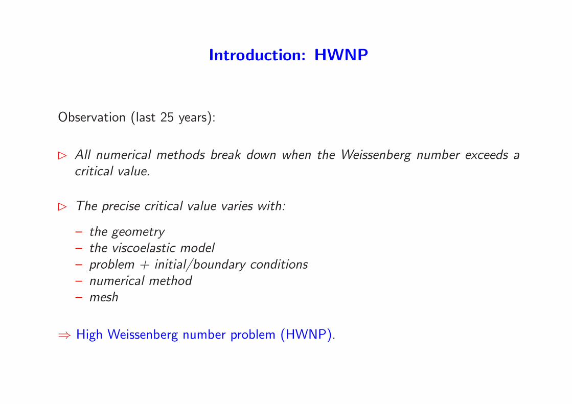
Introduction: HWNP

Observation (last 25 years):

⊲ All numerical methods break down when the Weissenberg number exceeds acritical value.

⊲ The precise critical value varies with:

– the geometry– the viscoelastic model– problem + initial/boundary conditions– numerical method– mesh

⇒ High Weissenberg number problem (HWNP).

Introduction: HWNP

⊲ It is still there, despite:

– ‘realistic’ constitutive models: pom-pom XPP FENE, FENE-P . . .

– advances in ‘stable’ computational methods SUPG DG DEVSS DEVSS-G/SUPG . . .

– application of various numerical discretization methods: FEM, FDM, SEM,spectral, . . .

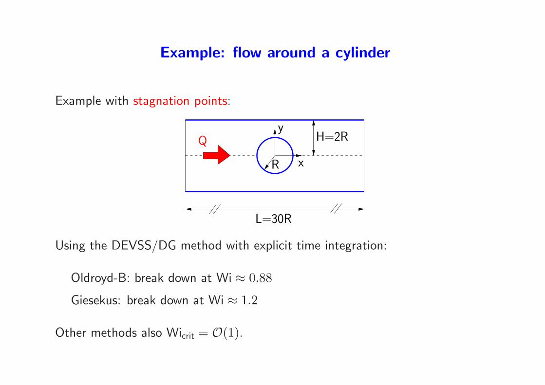
Example: flow around a cylinder

Example with stagnation points:

L=30R

xR

H=2Ry

Q

Using the DEVSS/DG method with explicit time integration:

Oldroyd-B: break down at Wi ≈ 0.88

Giesekus: break down at Wi ≈ 1.2

Other methods also Wicrit = O(1).

Example: 4:1 contraction

Example with geometrical singularities:

20R

20R

Q4R

R

Using the DEVSS/DG method with explicit time integration:

Phan-Thien/Tanner (linear factor) model: unsteady for Wi in the range20–30 with high-frequency stress oscillations in the downstream boundarylayer.

DEVSS/SUPG method typically fails with Wicrit = O(1).

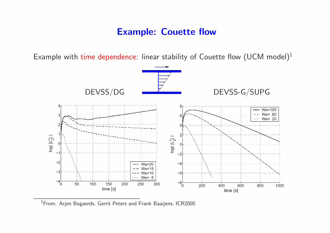
Example: Couette flow

Example with time dependence: linear stability of Couette flow (UCM model)1

DEVSS/DG DEVSS-G/SUPG

1From: Arjen Bogaerds, Gerrit Peters and Frank Baaijens, ICR2000

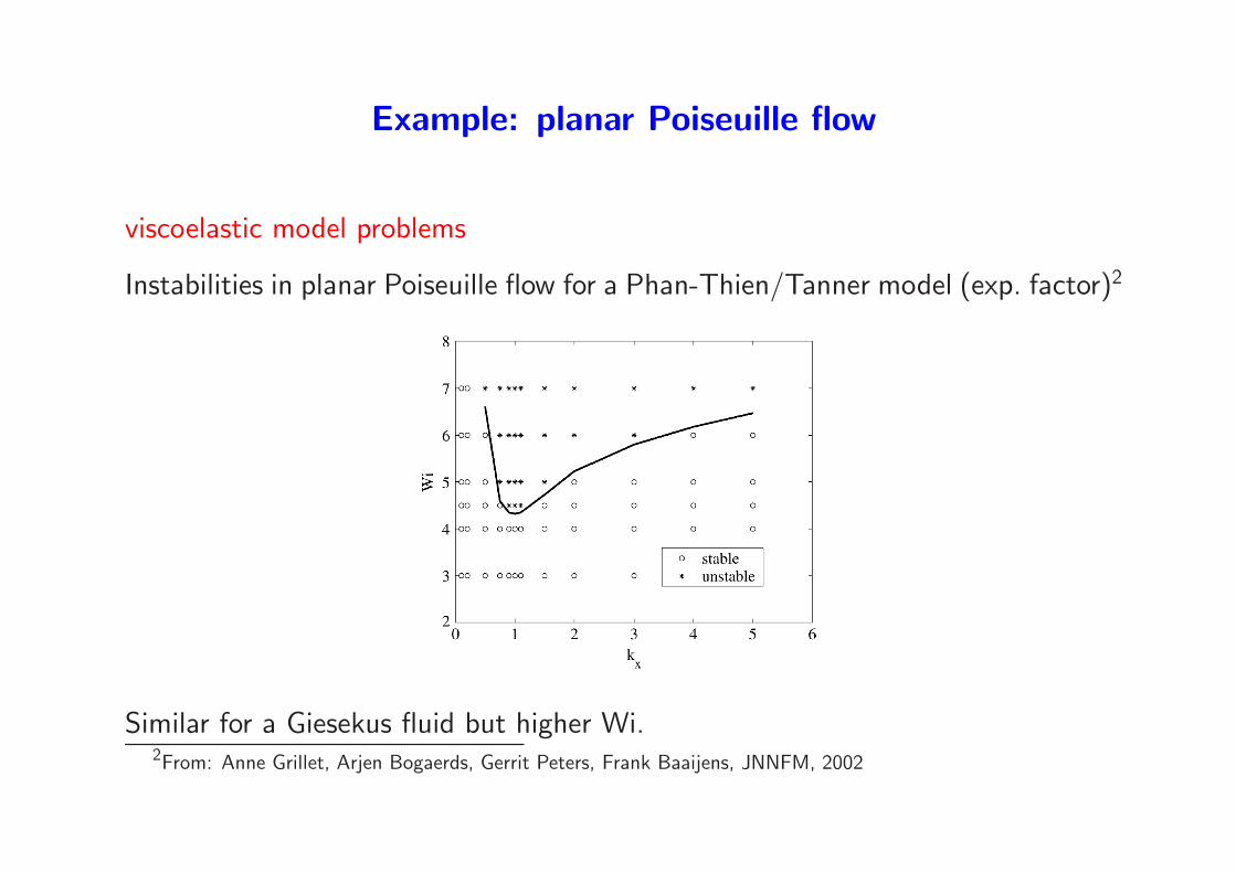
Example: planar Poiseuille flow

viscoelastic model problems

Instabilities in planar Poiseuille flow for a Phan-Thien/Tanner model (exp. factor)2

Similar for a Giesekus fluid but higher Wi.2From: Anne Grillet, Arjen Bogaerds, Gerrit Peters, Frank Baaijens, JNNFM, 2002

Example: rheometric functions

viscoelastic model problems

Steady planar elongational viscosity and steady shear stress (Giesekus):

1

10

100

1000

0.01 0.1 1 10 100 1000

(c11

-c22

)/λε•

λε•

α=0 (Oldroyd-B)α=0.01α=0.05

α=0.1

0.1

1

10

100

1000

0.1 1 10 100 1000c 1

2λγ•

α=0 (Oldroyd-B)α=0.01

α=0.1α=0.5α=0.7

12λ

ε

ε = ω (shear)

ω

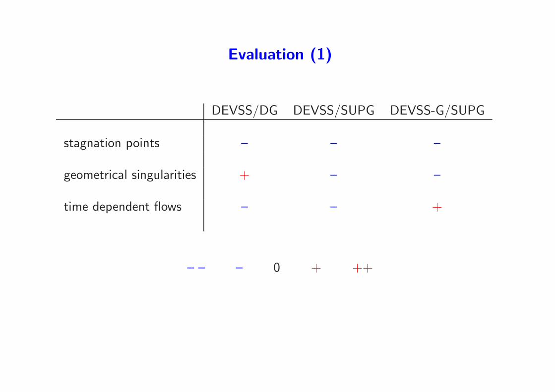
Evaluation (1)

DEVSS/DG DEVSS/SUPG DEVSS-G/SUPG

stagnation points – – –

geometrical singularities + – –

time dependent flows – – +

– – – 0 + ++

Evaluation (2)

The situation is quite different than classical CFD at large Reynolds numbers,where in most cases:

⊲ stable calculations can be performed, but

⊲ accuracy is lost due to insufficient mesh resolution.

Research efforts are directed towards fast and accurate numerical schemes on bigcomputers to solve problems for a better understanding of basic phenomena, suchturbulence.

⇒ The situation in Computational Rheology seems hopeless . . .

A new method

. . . until last year new hope has been raised:

Raanan Fattal & Raz Kupferman, JNNFM, 123, 281–285 (2004)

where:

⊲ a numerical instability related to exponential profiles at high Weissenbergnumber has been identified

⊲ a solution has been proposed

Outline

⊲ Basic equations & numerical methods

⊲ discuss the numerical instability for a simplified 1D model

⊲ a more ‘mechanical’ derivation of the newly proposed scheme

⊲ application to FEM using DEVSS/DG

⊲ evaluate the new approach for flows having

– stagnation points– geometrical singularities

⊲ Conclusions

Hulsen, Fattal & Kupferman, J. Non-Newtonian Fluid Mech., 127, 27-39, (2005)

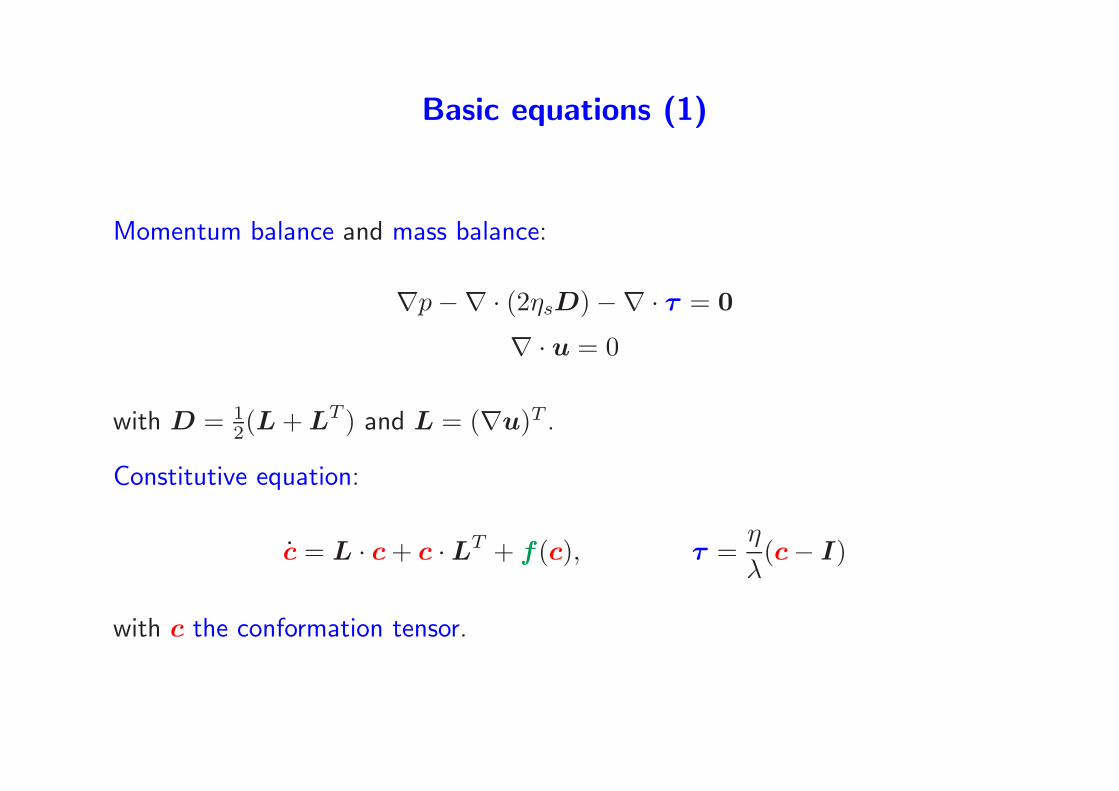
Basic equations (1)

Momentum balance and mass balance:

∇p−∇ · (2ηsD)−∇ · τ = 0

∇ · u = 0

with D = 12(L + LT ) and L = (∇u)T .

Constitutive equation:

c = L · c + c ·LT + f(c), τ =η

λ(c− I)

with c the conformation tensor.

Basic equations (2)

Expressions for f(c):

−λf (c) =

c− I Oldroyd-B

c− I + α(c− I)2 Giesekus

Y (tr c)(c− I

)Phan-Thien Tanner, with:

Y (tr c) =

1 + ǫ(tr c− 3) linear

exp[ǫ(tr c− 3)] exponential

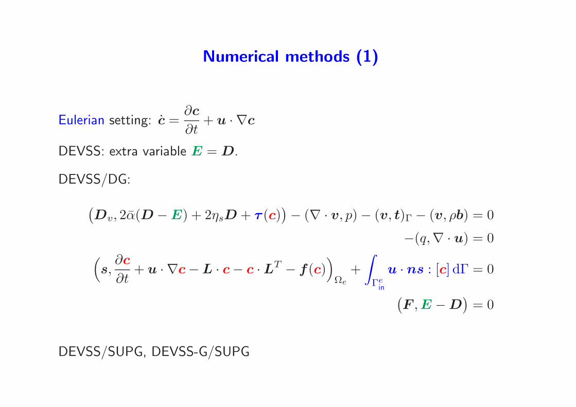
Numerical methods (1)

Eulerian setting: c =∂c

∂t+ u · ∇c

DEVSS: extra variable E = D.

DEVSS/DG:(Dv, 2α(D −E) + 2ηsD + τ (c)

)− (∇ · v, p)− (v, t)Γ − (v, ρb) = 0

−(q,∇ · u) = 0(s,

∂c

∂t+ u · ∇c−L · c− c ·LT − f(c)

)Ωe

+∫

Γein

u · ns : [c] dΓ = 0(F , E −D

)= 0

DEVSS/SUPG, DEVSS-G/SUPG

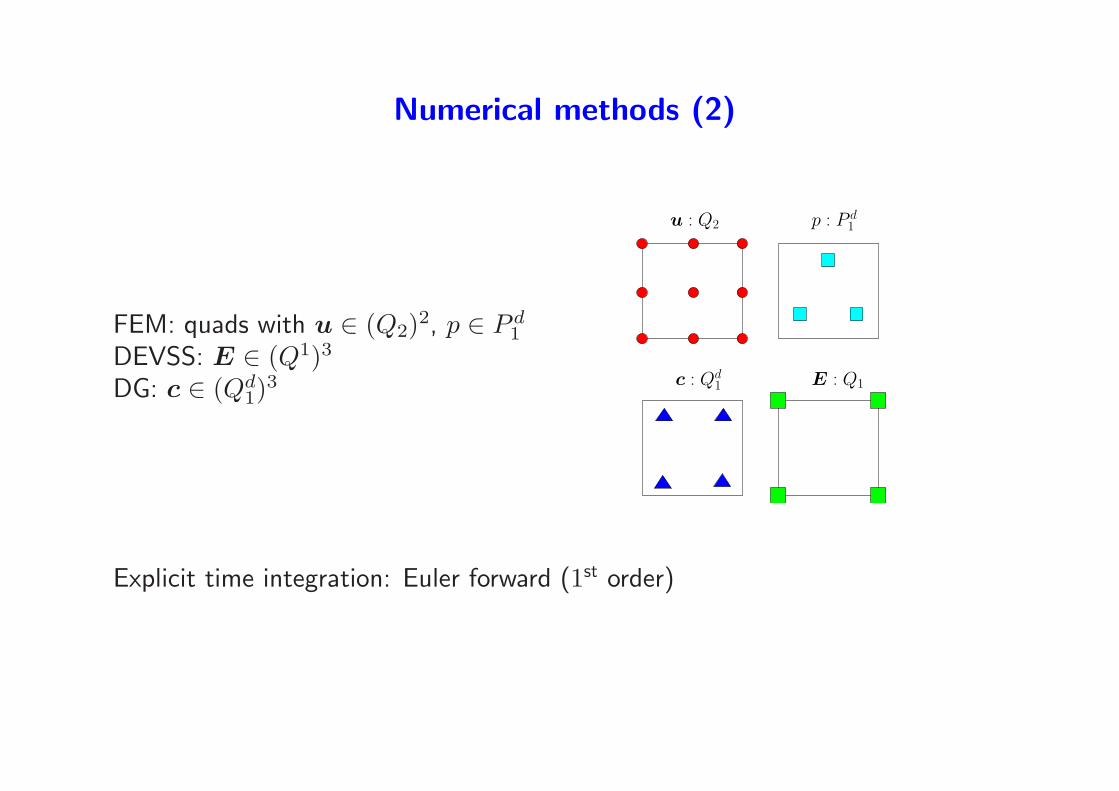
Numerical methods (2)

FEM: quads with u ∈ (Q2)2, p ∈ P d1

DEVSS: E ∈ (Q1)3

DG: c ∈ (Qd1)

3

u : Q2 p : P d1

c : Qd1 E : Q1

Explicit time integration: Euler forward (1st order)

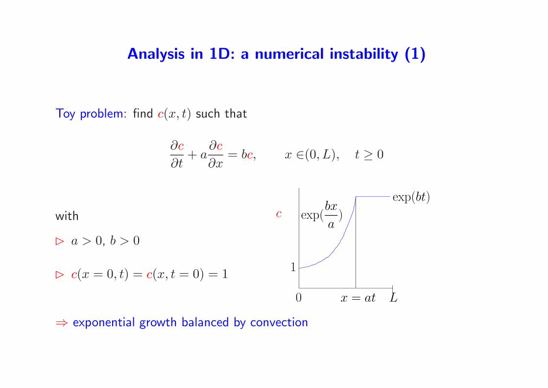
Analysis in 1D: a numerical instability (1)

Toy problem: find c(x, t) such that

∂c

∂t+ a

∂c

∂x= bc, x ∈(0, L), t ≥ 0

with

⊲ a > 0, b > 0

⊲ c(x = 0, t) = c(x, t = 0) = 1 1

exp(bx

a)

exp(bt)

0 x = at L

c

⇒ exponential growth balanced by convection

Analysis in 1D: a numerical instability (2)

Numerical discretization in space (first-orderupwind):

dci

dt= −a

ci − ci−1

∆x+ bci

= (b− a

∆x)ci +

a

∆xci−1

ci−1

ci

ci+1

i− 2 i− 1 i + 1i

∆x

ci−2

or in matrix formdc

dt= Ac

with

A =

γ 0β γ

. . . . . .0 β γ

, γ = b− a

∆x, β =

a

∆x

Analysis in 1D: a numerical instability (3)

To avoid exponential growth in time:

γ = b− a

∆x≤ 0 or ∆x ≤ a

b

Define C:

C =∆xb

athen for stability:

C ≤ 1 first-order upwind

For DG using linear polynomials:

C ≤ 2 DG with P1

⇒ Failure to balance exponential growth with convection when criterion violated.

Analysis in 1D: a numerical instability (4)

For Oldroyd-B in extension: a = u, b = 2ǫ− 1λ, with ǫ =

∂u

∂x:

C =∆x max(2ǫ− 1

λ, 0)

|u|

For Giesekus in extension: a = u, b = 2ǫ− 1λ(1 + 2αcxx),

C =∆x max(2ǫ− 1

λ(1 + 2αcxx), 0)

|u|

Solution to the problem: log transformation

Solution: solve for s = log c.

PDE for s:

s =c

c=

bc

c= b

with s =∂s

∂t+ a

∂s

∂x, and thus:

∂s

∂t+ a

∂s

∂x= b, x ∈(0, L), t ≥ 0

and c = exp(s).

1

0 x = at L

btbx

a

s

⇒ No numerical instability. No restrictions on ∆x

Log transformation for tensors

log τij?: No

log τ?: No

log cij?: No

log c: YES!

Thus we choose s = log c.

BONUS: c = exp(s) always positive definite!.

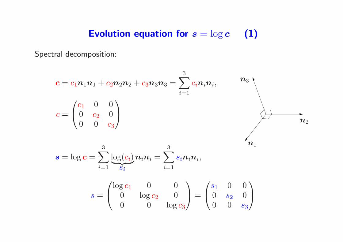
Evolution equation for s = log c (1)

Spectral decomposition:

c = c1n1n1 + c2n2n2 + c3n3n3 =3∑

i=1

cinini,

c =

c1 0 00 c2 00 0 c3

s = log c =3∑

i=1

log(ci)︸ ︷︷ ︸si

nini =3∑

i=1

sinini,

n2

n3

n1

s =

log c1 0 00 log c2 00 0 log c3

=

s1 0 00 s2 00 0 s3

Evolution equation for s = log c (2)

Substantial derivative of s:

s =3∑

i=1

sinini +3∑

i=1

sinini +3∑

i=1

sinini

or with si =d(log ci)

dt=

ci

ci

s =3∑

i=1

ci

cinini +

3∑i=1

sinini +3∑

i=1

sinini

⇒ We need expressions for ci and ni

Evolution equation for s = log c (3)

We get ci and ni from the CE:

c = L · c + c ·LT + f(c)

From the diagonal components (in the ni-frame):

ci = 2ciLii + fi(c1, c2, c3)

From the off-diagonal components (in the ni-frame):

ni = ω · ni =3∑

j=1

ωjinj

n2

n3

n1

n2

n3

n1

with the components ωij of the skewsymmetric tensor ω:

ωij =ciLji + cjLij

cj − ci, i 6= j, ci 6= cj

Evolution equation for s = log c (4)

End result:

s = 23∑

i=1

Liinini +3∑

i=1

fi(c1, c2, c3)ci

nini︸ ︷︷ ︸diagonal

+3∑

i=1

3∑j=1

i 6=j

si − sj

ci − cj(cjLij + ciLji)ninj

︸ ︷︷ ︸off-diagonal

Notes:

⊲ ci = exp(si), c = exp(s)

⊲ limci→cj

si − sj

ci − cj(cjLij + ciLji) = Lij + Lji = 2Dij

Numerical implementation

⊲ Easy to implement in an existing code based on explicit time integration forthe right-hand side of the evolution equation for s.

⊲ Additional operations required:

– Fast routine for eigenvalues and eigenvectors for 2×2 (2D) and 3×3 (3D)matrices.

– Transformation of tensors between the global and principal system.

⊲ Treatment of convection term identical to the standard scheme.

⊲ Fully implicit time integration or Newton-Raphson like procedure are muchmore difficult to implement than in the standard scheme.

Flow past a cylinder confined between two flat plates

⊲ Oldroyd-B model with ηs/η = 0.59,where η = ηs + ηp

⊲ Giesekus model with α = 0.01.

⊲ Weissenberg number: Wi =λU

R,

with U average velocity in channel.

⊲ Dimensionless drag force K =Fx

ηU

L=30R

xR

H=2Ry

Q

⊲ Dimensionless scaling: coordinates with R, stresses withηU

R, time with R/U ,

velocities with U .

⊲ Periodical boundary conditions.

Rheology of Giesekus model with α = 0.01

0.01

0.1

1

10

0.1 1 10 100 1000

c 12/

λγ•

λγ•

α=0.01

0.01

0.1

1

10

0.1 1 10 100 1000

η/η 0

λγ•

α=0.01

0.1

1

10

100

0.1 1 10 100 1000

(c11

-c22

)/2c

12

λγ•

α=0.01

1

10

100

1000

0.01 0.1 1 10 100

(c11

-c22

)/λε•

λε•

α=0.01

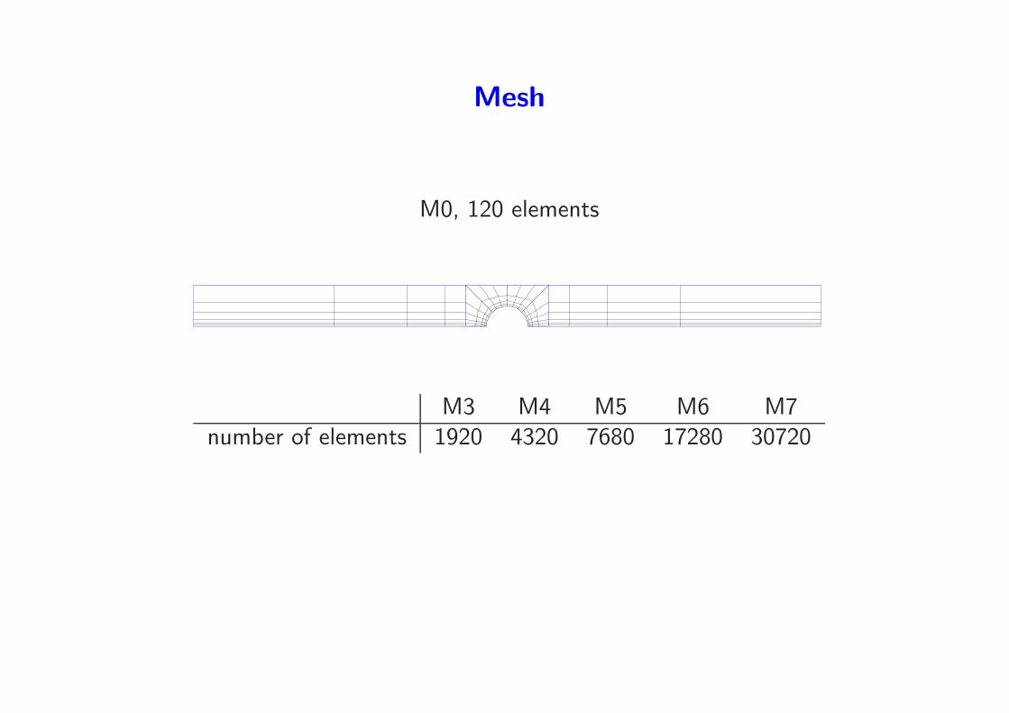
Mesh

M0, 120 elements

M3 M4 M5 M6 M7number of elements 1920 4320 7680 17280 30720

Value of C on the center line in the wake for Oldroyd-B

0

0.5

1

1.5

2

2.5

3

3.5

4

4.5

5

1 1.1 1.2

C

x

Wi=0.7Wi=0.86Wi=0.87Wi=0.88, time=18Wi=1.0, matrix logarithm

Value of C on the center line in the wake for Giesekus

0

0.5

1

1.5

2

2.5

3

3.5

1 1.1 1.2

C

x

Wi=1.17Wi=1.18Wi=1.19

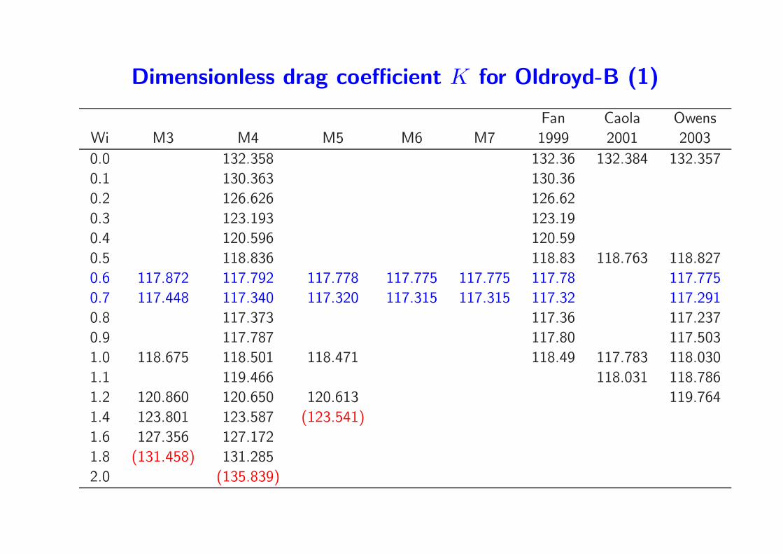
Dimensionless drag coefficient K for Oldroyd-B (1)

Fan Caola Owens

Wi M3 M4 M5 M6 M7 1999 2001 2003

0.0 132.358 132.36 132.384 132.357

0.1 130.363 130.36

0.2 126.626 126.62

0.3 123.193 123.19

0.4 120.596 120.59

0.5 118.836 118.83 118.763 118.827

0.6 117.872 117.792 117.778 117.775 117.775 117.78 117.775

0.7 117.448 117.340 117.320 117.315 117.315 117.32 117.291

0.8 117.373 117.36 117.237

0.9 117.787 117.80 117.503

1.0 118.675 118.501 118.471 118.49 117.783 118.030

1.1 119.466 118.031 118.786

1.2 120.860 120.650 120.613 119.764

1.4 123.801 123.587 (123.541)

1.6 127.356 127.172

1.8 (131.458) 131.285

2.0 (135.839)

Dimensionless drag coefficient K for Oldroyd-B (2)

116

118

120

122

124

126

128

130

132

134

0 0.2 0.4 0.6 0.8 1 1.2 1.4 1.6 1.8

dim

ensi

onle

ss d

rag

coef

ficie

nt K

Wi

DG, matrix logarithm, mesh M4Fan et al.Caola et al.Owens et al.

Minimum value of det c

0

1

2

3

4

5

6

7

-15 -10 -5 0 5 10 15

log(

det c

)

x

Wi=1.8, M4

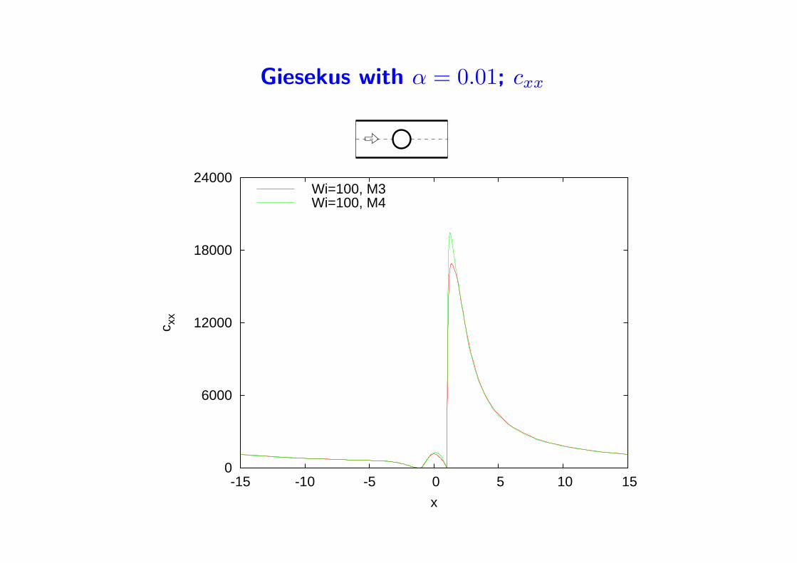
Giesekus with α = 0.01; cxx

0

6000

12000

18000

24000

-15 -10 -5 0 5 10 15

c xx

x

Wi=100, M3Wi=100, M4

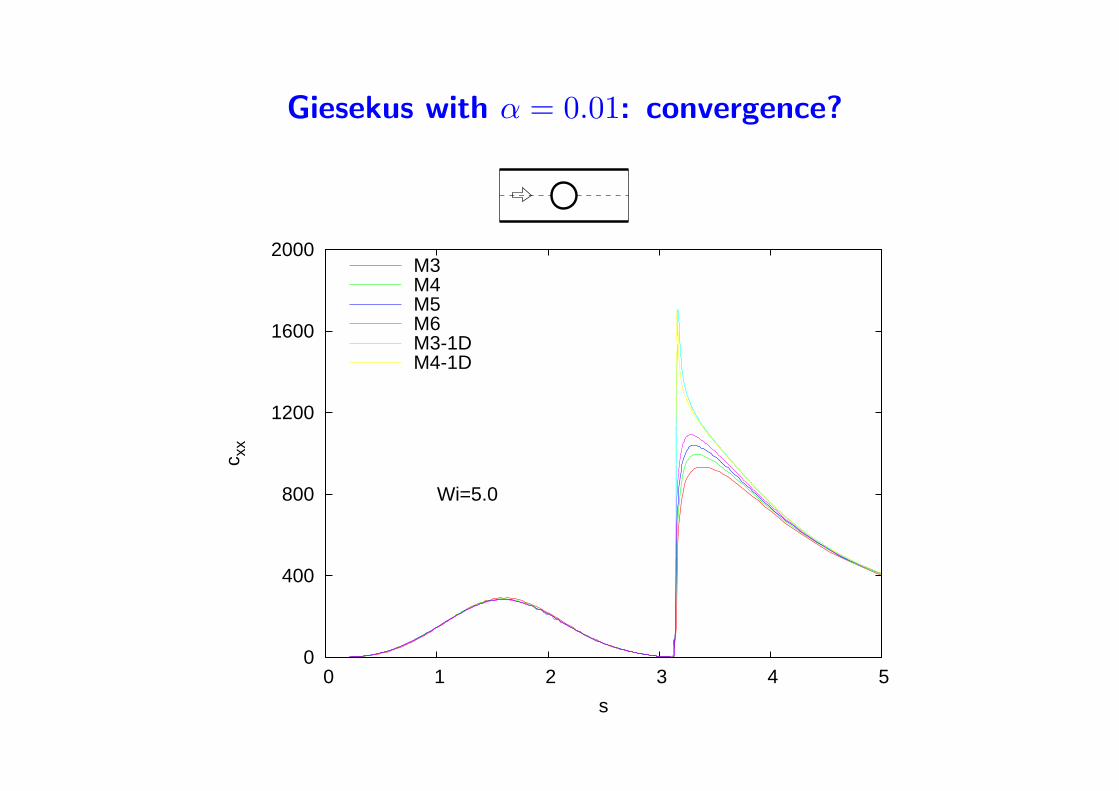
Giesekus with α = 0.01: convergence?

0

400

800

1200

1600

2000

0 1 2 3 4 5

c xx

s

Wi=5.0

M3M4M5M6M3-1DM4-1D

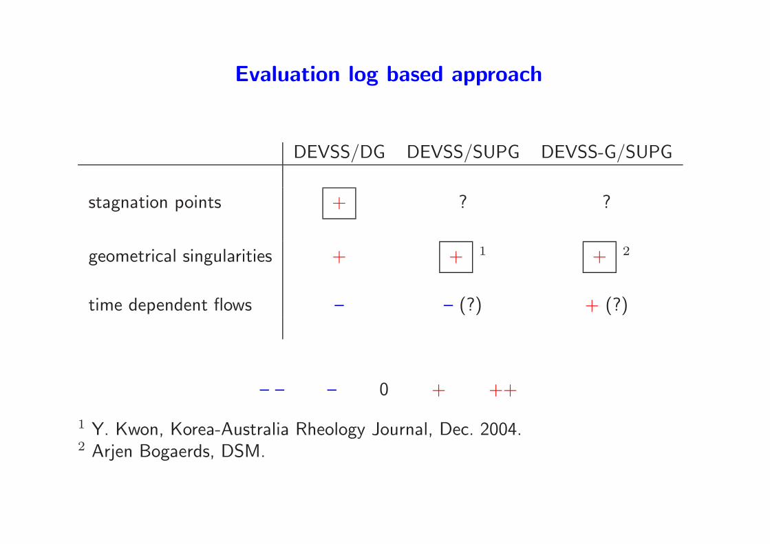
Evaluation log based approach

DEVSS/DG DEVSS/SUPG DEVSS-G/SUPG

stagnation points + ? ?

geometrical singularities + + 1 + 2

time dependent flows – – (?) + (?)

– – – 0 + ++

1 Y. Kwon, Korea-Australia Rheology Journal, Dec. 2004.2 Arjen Bogaerds, DSM.

Evaluation log based approach (currently 2007)

DEVSS/DG DEVSS/SUPG DEVSS-G/SUPG

stagnation points + ? +

geometrical singularities + + 1 + 2

time dependent flows – – (?) +

– – – 0 + ++

1 Y. Kwon, Korea-Australia Rheology Journal, Dec. 2004.2 Arjen Bogaerds, DSM.

Conclusions

⊲ The log conformation transformation can stabilize viscoelastic computationsin a major way. This supports the idea that in many problems the numericalinstability due to exponential profiles is the limiting factor.

⊲ It does not resolve the spurious linear instabilities in Couette flow. Obviouslyit does not solve other problems like inherent problems with the CE. Thereforethe amount of stabilization depends on the ‘weakest link’.

⊲ In regions with exponential profiles serious questions remain on convergenceof the solution with mesh refinement. (see also: “Guenette et al., J. Non-Newtonian Fluid Mech., 153, (2008) 34-45).

⊲ For now, the DEVSS-G/SUPG scheme combined with the log transformationseems to be the best candidate to solve time-dependent/stability problems athigh Weissenberg number.

References (1)

Recent general reviews:

Frank P.T. Baaijens, Martien A. Hulsen, Patrick D. Anderson The Use of MixedFinite Element Methods for Viscoelastic Fluid Flow Analysis Encyclopedia OfComputational Mechanics. Editors Erwin Stein, Rene de Borst and Thomas J.R.Hughes. Volume 3 Fluids∗

R.G. Owens & T.N. Philips: “Computational Rheology”, Imperial College Press,London, 2002.

R. Keunings: A Survey of Computational Rheology, Plenary Lecture, Proc. 13thInt. Congr. on Rheoloy, Cambridge, D.M. Binding et al. (Eds), British Society ofRheology, Glasgow, Vol. 1, 7-14 (2000)∗

F.P.T. Baaijens: “Mixed finite element methods for viscoelastic flow analysis: Areview”, J. Non-Newtonian Fluid Mech. 79 (1998) 361-385∗

∗ (downloadable from website of this course).

References (2)

Review on using integral viscoelastic fluid models:

R. Keunings, Finite Element Methods for Integral Viscoelastic Fluids, in RheologyReviews 2003, D.M. Binding and K. Walters (Eds.), British Society of Rheology,167-195 (2003)

Review on micro-macro methods:

R. Keunings, Micro-Macro Methods for the Multiscale Simulation of ViscoelasticFlow using Molecular Models of Kinetic Theory, to appear in Rheology Reviews2004, D.M. Binding and K. Walters (Eds.), British Society of Rheology (2004)

Note: The reviews of Roland Keunings are downloadable from his website:http://www.inma.ucl.ac.be/˜rk/getpapers.html.

References (3)

Paper on log transformation:

Martien A. Hulsen, Raanan Fattal, Raz Kupferman “Flow of viscoelastic fluidspast a cylinder at high Weissenberg number: stabilized simulations using matrixlogarithms”, J. Non-Newtonian Fluid Mech., 127 (2005) 27–39∗

Introduction to FEM, FDM, FVM, minimization problems:

J. van Kan, G. Segal and F. Vermolen: “Numerical Methods in ScientificComputing”, VSSD, Delft, The Netherlands, 2005.

Finite element methods for flow problems:

J. Donea and A. Huerto: “Finite Element Methods for Flow Problems”, JohnWiley & Sons, Chichester, 2003.

P.M. Gresho and R.L. Sani: “Incompressible Flow and the Finite ElementMethod”, Volumes 1 and 2, John Wiley, New York, 2000.

∗ (downloadable from website of this course).