Confidence Interval Estimation

For statistical inference in

decision making:

Objectives

• Central Limit Theorem• Confidence Interval Estimation of the

Mean (σ known)• Interpretation of the Confidence Interval• Confidence Interval Estimation of the

Mean (σ unknown)• Confidence Interval Estimation for the

Proportion• Determining Sample Size

Central Limit Theorem

Irrespective of the shape of the underlying distribution of the population, by increasing the sample size, sample means & proportions will approximate normal distributions if the sample sizes are sufficiently large.

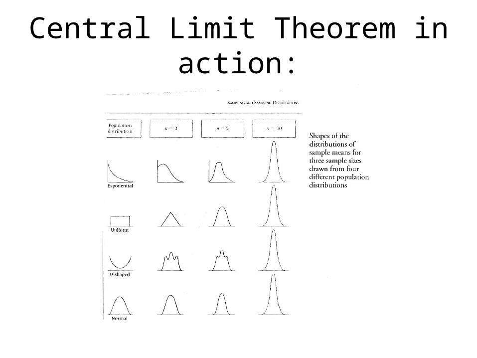
Central Limit Theorem in action:

How large must a sample be for the Central Limit theorem to apply?

The sample size varies according to the shape of the population.

However, for our use, a sample size of 30 or larger will suffice.

Must sample sizes be 30 or larger for populations that are normally distributed?

No. If the population is normally distributed, the sample means are normally distributed for sample sizes as small as n=1.

Why not just always pick a sample size of 30?

How can I tell the shape of the underlying population?

• CHECK FOR NORMALITY:• Use descriptive statistics. Construct stem-and-leaf plots for small

or moderate-sized data sets and frequency distributions and histograms for large data sets.

• Compute measures of central tendency (mean and median) and compare with the theoretical and practical properties of the normal distribution. Compute the interquartile range. Does it approximate the 1.33 times the standard deviation?

• How are the observations in the data set distributed? Do approximately two thirds of the observations lie between the mean and plus or minus 1 standard deviation? Do approximately four-fifths of the observations lie between the mean and plus or minus 1.28 standard deviations? Do approximately 19 out of every 20 observations lie between the mean and plus or minus 2 standard deviations?

Why do I care if X-bar, the sample mean, is normally distributed?

Because I want to use Z scores to analyze sample means.

But to use Z scores, the data must be normally distributed.

That’s where the Central Limit Theorem steps in.

Recall that the Central Limit Theorem states that sample means are normally distributed regardless of the shape of the underlying population if the sample size is sufficiently large.

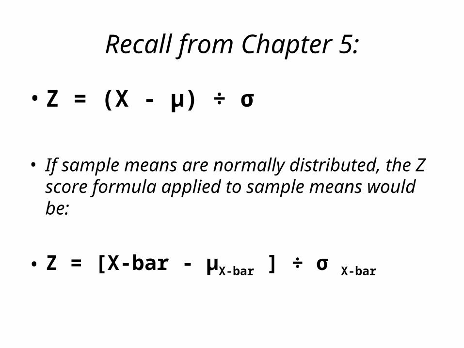
Recall from Chapter 5:

• Z = (X - µ) ÷ σ

• If sample means are normally distributed, the Z score formula applied to sample means would be:

• Z = [X-bar - µX-bar ] ÷ σ X-bar

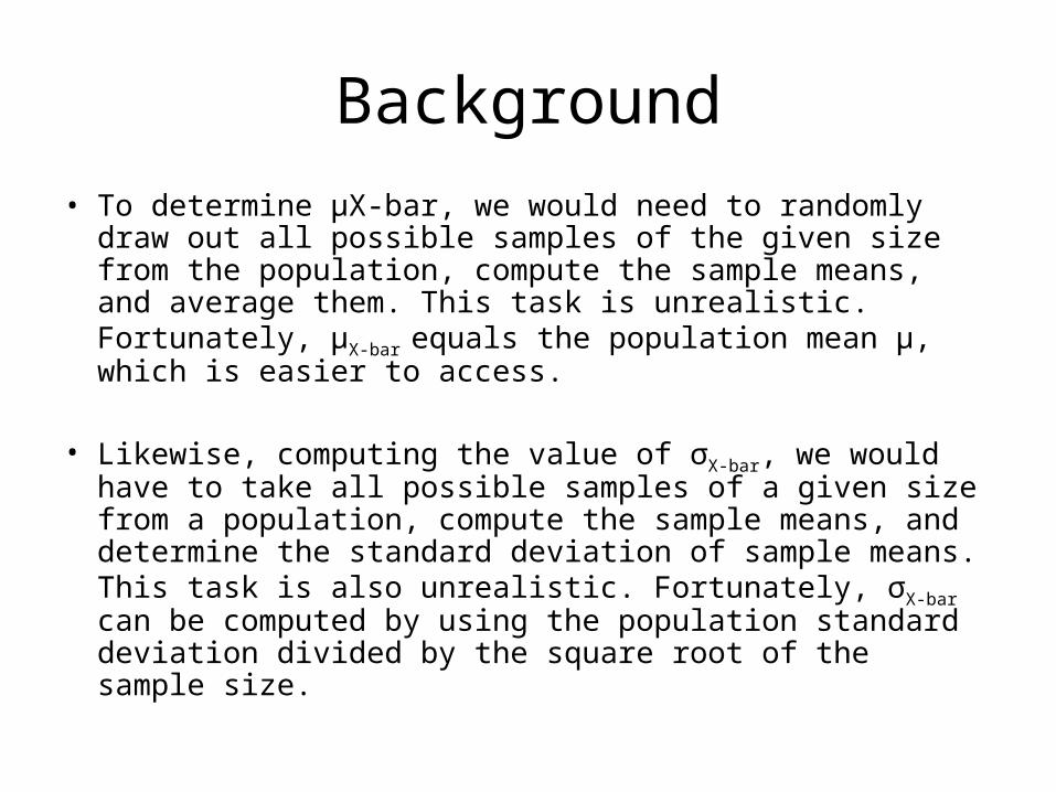
Background

• To determine µX-bar, we would need to randomly draw out all possible samples of the given size from the population, compute the sample means, and average them. This task is unrealistic. Fortunately, µX-bar equals the population mean µ, which is easier to access.

• Likewise, computing the value of σX-bar, we would have to take all possible samples of a given size from a population, compute the sample means, and determine the standard deviation of sample means. This task is also unrealistic. Fortunately, σX-bar can be computed by using the population standard deviation divided by the square root of the sample size.

Note:

As the sample size increases,

the standard deviation of the sample means becomes smaller and smaller

because the population standard deviation is being divided by larger and larger values of the square root of n.

The ultimate benefit of the central limit theorem is a useful version of the Z formula for sample means.

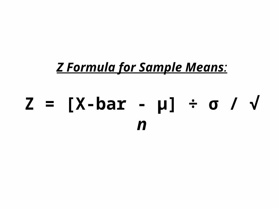
Z Formula for Sample Means:

Z = [X-bar - µ] ÷ σ / √ n

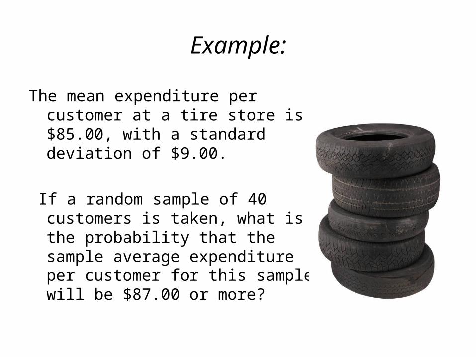
Example:

The mean expenditure per customer at a tire store is $85.00, with a standard deviation of $9.00.

If a random sample of 40 customers is taken, what is the probability that the sample average expenditure per customer for this sample will be $87.00 or more?

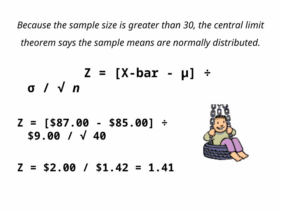
Because the sample size is greater than 30, the central limit theorem says the sample means are normally

distributed.

Z = [X-bar - µ] ÷ σ / √ n

Z = [$87.00 - $85.00] ÷ $9.00 / √ 40

Z = $2.00 / $1.42 = 1.41

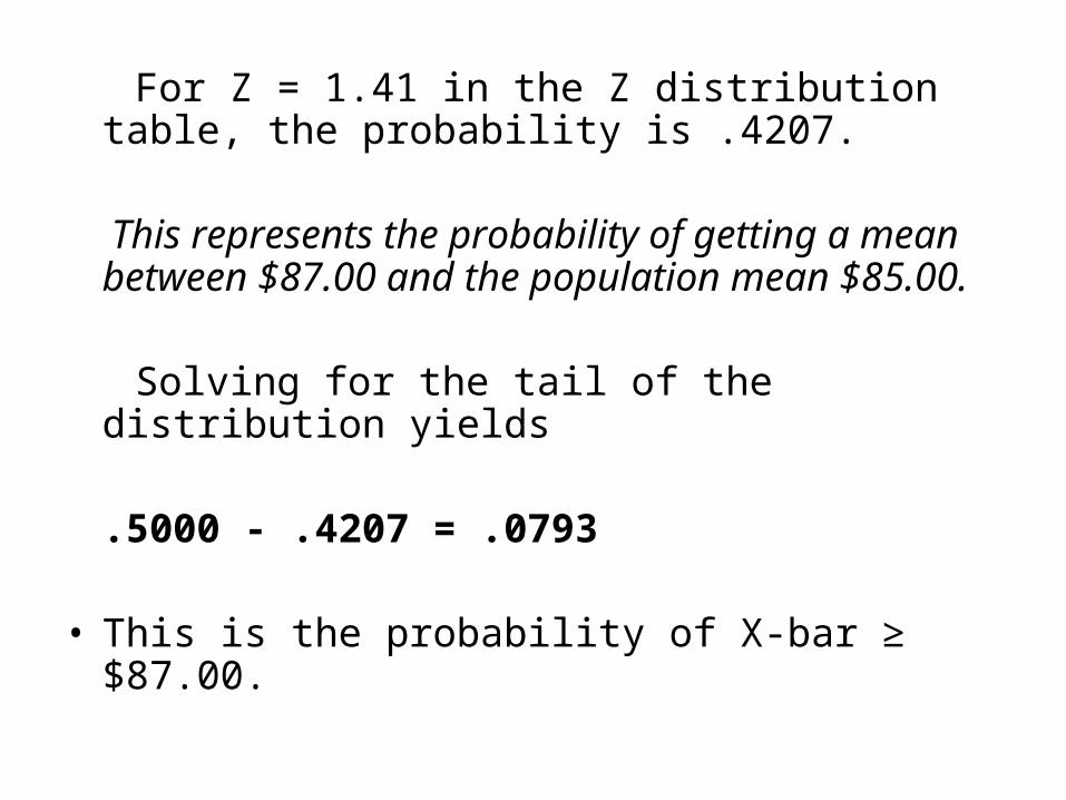
For Z = 1.41 in the Z distribution table, the probability is .4207.

This represents the probability of getting a mean between $87.00 and the population mean $85.00.

Solving for the tail of the distribution yields

.5000 - .4207 = .0793

• This is the probability of X-bar ≥ $87.00.

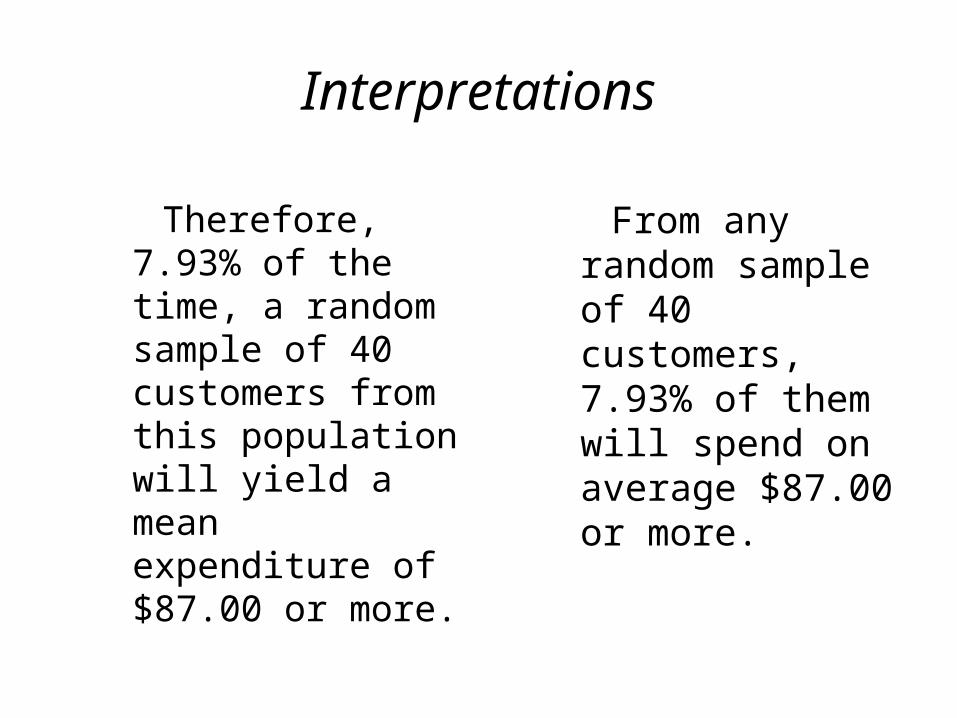
Interpretations

Therefore, 7.93% of the time, a random sample of 40 customers from this population will yield a mean expenditure of $87.00 or more.

OR

From any random sample of 40 customers, 7.93% of them will spend on average $87.00 or more.

Interpretations

Therefore, 7.93% of the time, a random sample of 40 customers from this population will yield a mean expenditure of $87.00 or more.

From any random sample of 40 customers, 7.93% of them will spend on average $87.00 or more.

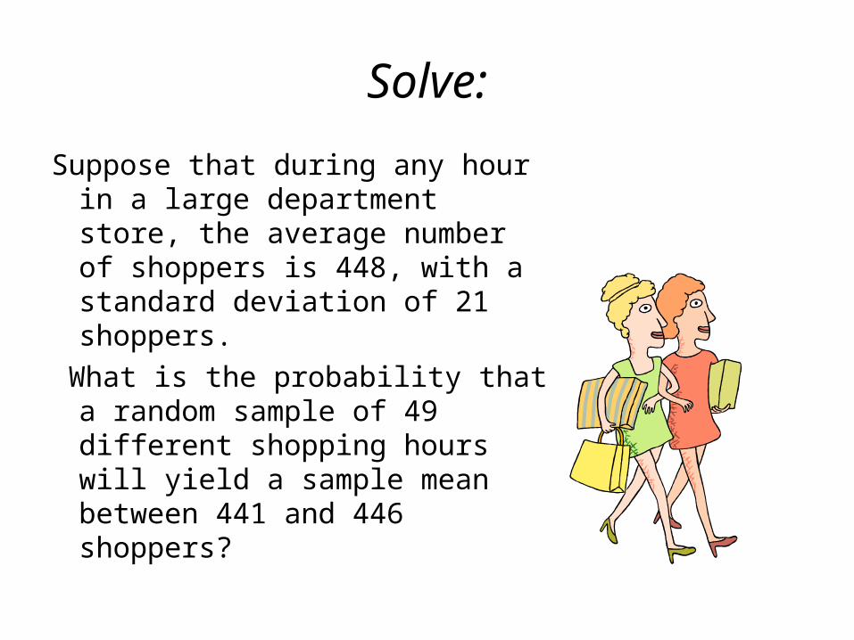
Solve:

Suppose that during any hour in a large department store, the average number of shoppers is 448, with a standard deviation of 21 shoppers.

What is the probability that a random sample of 49 different shopping hours will yield a sample mean between 441 and 446 shoppers?

Statistical Inference

Statistical Inference facilitates decision making.

Via sample data,

we can estimate something about our population,

such as its average value µ,

by using the corresponding sample mean, X-bar.

Recall that µ,

the population mean to be estimated,

is a parameter,

while X-bar, the sample mean, is a statistic.

Point Estimate

A point estimate is a statistic taken from a sample and is used to estimate a population parameter.

However, a point estimate is only as good as the sample it represents. If other random samples are taken from the population, the point estimates derived from those samples are likely to vary.

Because of variation in sample statistics, estimating a population parameter with a confidence interval is often preferable to using a point estimate.

Confidence Interval

A confidence interval is a range of values within which it is estimated with some confidence the population parameter lies.

Confidence intervals can be one or two-tailed.

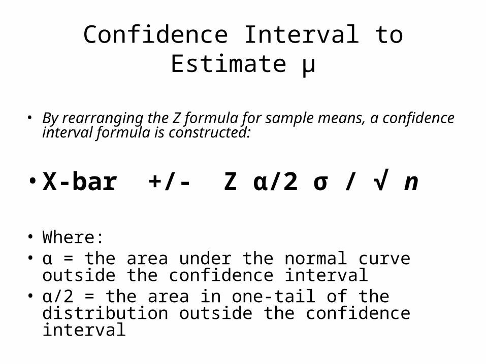
Confidence Interval to Estimate µ

• By rearranging the Z formula for sample means, a confidence interval formula is constructed:

• X-bar +/- Z α/2 σ / √ n

• Where:• α = the area under the normal curve outside the

confidence interval• α/2 = the area in one-tail of the distribution outside

the confidence interval

The confidence interval formula yields a range (interval) within which we feel with some confidence the population mean is located.

It is not certain that the population mean is in the interval unless we have a 100% confidence interval that is infinitely wide, so wide that it is meaningless.

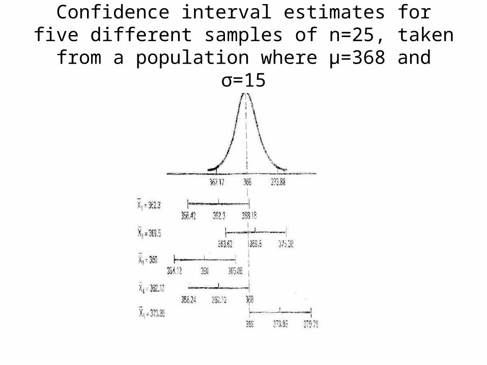
Confidence interval estimates for five different samples of n=25, taken from a population where

µ=368 and σ=15

Common levels of confidence intervals used by analysts are

90%, 95%, 98%, and 99%.

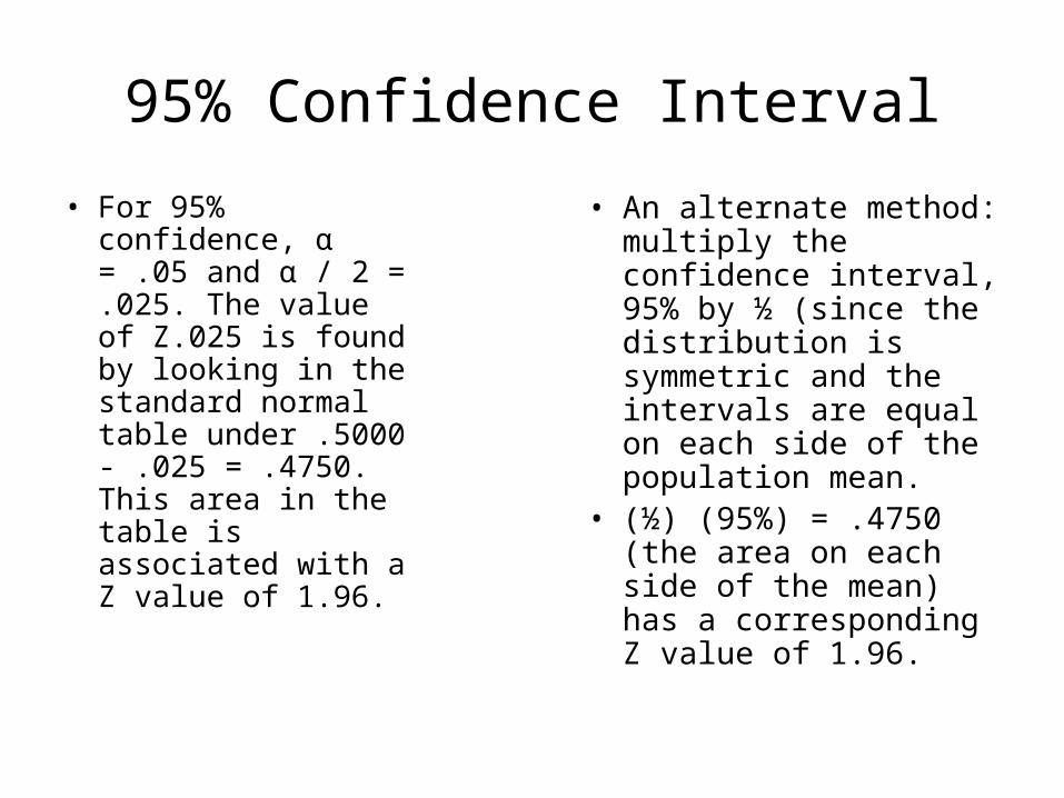
95% Confidence Interval

• For 95% confidence, α = .05 and α / 2 = .025. The value of Z.025 is found by looking in the standard normal table under .5000 - .025 = .4750. This area in the table is associated with a Z value of 1.96.

• An alternate method: multiply the confidence interval, 95% by ½ (since the distribution is symmetric and the intervals are equal on each side of the population mean.

• (½) (95%) = .4750 (the area on each side of the mean) has a corresponding Z value of 1.96.

In other words, of all the possible X-bar values along the horizontal axis of the normal distribution curve, 95% of them should be within a Z score of 1.96 from

the mean.

Margin of Error

Z [σ / √ n]

Example:

• A business analyst for cellular telephone company takes a random sample of 85 bills for a recent month and from these bills computes a sample mean of 153 minutes. If the company uses the sample mean of 153 minutes as an estimate for the population mean, then the sample mean is being used as a POINT ESTIMATE. Past history and similar studies indicate that the population standard deviation is 46 minutes.

• The value of Z is decided by the level of confidence desired. A confidence level of 95% has been selected.

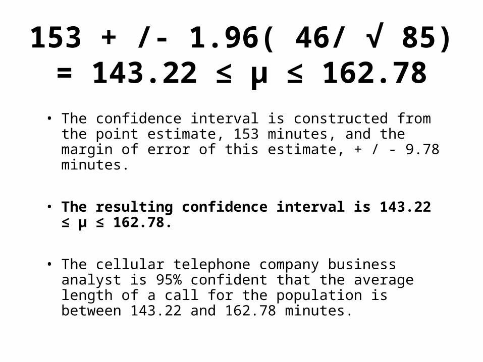
153 + /- 1.96( 46/ √ 85)= 143.22 ≤ µ ≤ 162.78

• The confidence interval is constructed from the point estimate, 153 minutes, and the margin of error of this estimate, + / - 9.78 minutes.

• The resulting confidence interval is 143.22 ≤ µ ≤ 162.78.

• The cellular telephone company business analyst is 95% confident that the average length of a call for the population is between 143.22 and 162.78 minutes.

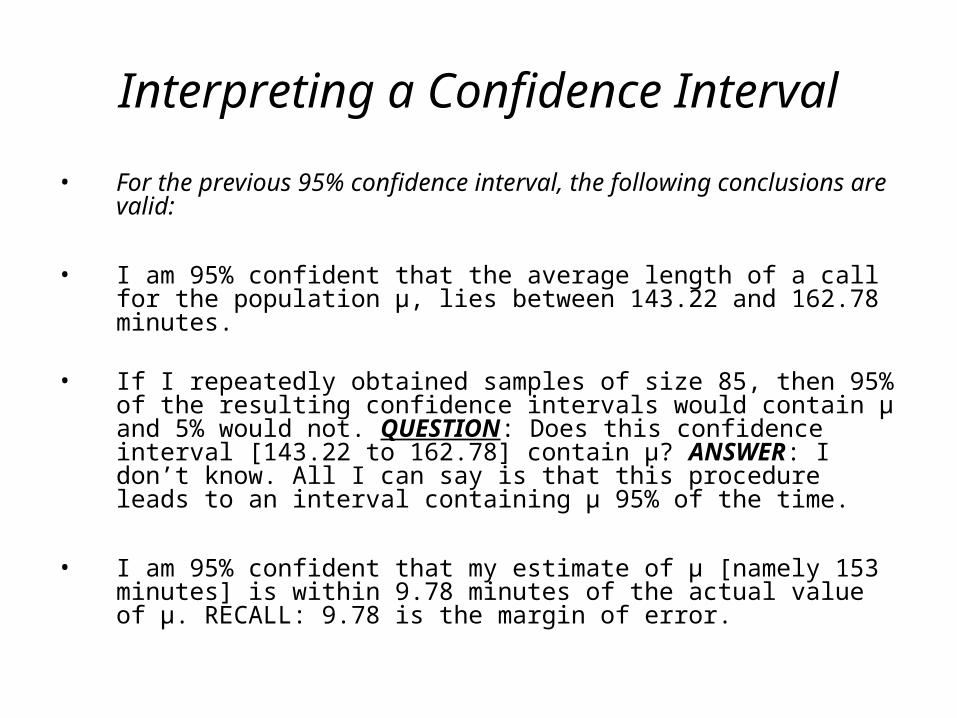
Interpreting a Confidence Interval

• For the previous 95% confidence interval, the following conclusions are valid:

• I am 95% confident that the average length of a call for the population µ, lies between 143.22 and 162.78 minutes.

• If I repeatedly obtained samples of size 85, then 95% of the resulting confidence intervals would contain µ and 5% would not. QUESTION: Does this confidence interval [143.22 to 162.78] contain µ? ANSWER: I don’t know. All I can say is that this procedure leads to an interval containing µ 95% of the time.

• I am 95% confident that my estimate of µ [namely 153 minutes] is within 9.78 minutes of the actual value of µ. RECALL: 9.78 is the margin of error.

Be Careful! The following statement is NOT true:

“The probability that µ lies between 143.22 and 162.78 is .95.”

Once you have inserted your sample results into the confidence interval formula, the word PROBABILITY can no longer be used to describe the resulting confidence interval.