Conditional Hardness for Approximate Coloring

Irit Dinur∗ Elchanan Mossel† Oded Regev‡

November 3, 2005

Abstract

We study theAPPROXIMATE-COLORING(q,Q) problem: Given a graphG, decide whetherχ(G) ≤ qor χ(G) ≥ Q (whereχ(G) is the chromatic number ofG). We derive conditional hardness for thisproblem for any constant3 ≤ q < Q. For q ≥ 4, our result is based on Khot’s2-to-1 conjecture[Khot’02]. For q = 3, we base our hardness result on a certain ‘⊲< shaped’ variant of his conjecture.

We also prove that the problemALMOST-3-COLORINGε is hard for any constantε > 0, assumingKhot’s Unique Games conjecture. This is the problem of deciding for a given graph, between the casewhere one can3-color all but aε fraction of the vertices without monochromatic edges, and the casewhere the graph contains no independent set of relative sizeat leastε.

Our result is based on bounding various generalized noise-stability quantities using the invarianceprinciple of Mossel et al [MOO’05].

∗Hebrew University. Email:dinuri@cs.huji.ac.il. Supported by the Israel Science Foundation and by BSF grant2004105

†Statistics, U.C. Berkeley. Email:mossel@stat.berkeley.edu. Supported by a Miller fellowship in Computer Scienceand Statistics, by a Sloan fellowship in Mathematics, by NSFgrants DMS-0504245, DMS-0528488 and by BSF grant 2004105

‡Department of Computer Science, Tel-Aviv University, Tel-Aviv 69978, Israel. Supported by an Alon Fellowship, by the IsraelScience Foundation and by BSF grant 2004105

1 Introduction

For a graphG = (V,E) we letχ(G) be the chromatic number ofG, i.e., the smallest number of colorsneeded to color the vertices ofG without monochromatic edges. We study the following problem,

APPROXIMATE -COLORING (q,Q) : Given a graphG, decide betweenχ(G) ≤ q andχ(G) ≥ Q.

The problemAPPROXIMATE-COLORING(3, Q) is notorious for the wide gap between the value ofQ forwhich an efficient algorithm is known and that for which a hardness result exists. The best known polynomial-time algorithm solves the problem forQ = O(n3/14) colors, wheren is the number of vertices [3] (In fact,that algorithm solves thesearch problemof finding aQ-coloring given aq-colorable graph. Since we aremainly interested in hardness results, we restrict our attention to the decision version of the problem). Incontrast, the strongest known hardness result shows that the problem is NP-hard forQ = 5 [12, 8]. Thus,the problem is open for all5 < Q < O(n3/14). In this paper we give some evidence that this problem ishard for any constant value ofQ. We remark that any hardness result forq = 3 immediately carries over forall q > 3.

The best algorithm known for larger values ofq is due to Halperin et al. [9], improving on a previousresult of Karger et al [11]. Their algorithm solvesAPPROXIMATE-COLORING(q,Q) for Q = nαq where0 < αq < 1 is some function ofq. For example,α4 ≈ 0.37. Improving on an earlier result of Furer [7],

Khot has shown [13] that for any large enough constantq andQ = qlog q25 , APPROXIMATE-COLORING(q,Q)

is NP-hard. A related problem is that of approximating the chromatic numberχ(·) of a given graph. For thisproblem, an inapproximability result ofn1−o(1) is known [6, 13].

Constructions: Our constructions follow the standard composition paradigm initiated in [2, 10], whichhas yielded numerous inapproximability results by now. In our context, this means that we show reductionsfrom variants of a problem known as label-cover to approximate graph coloring problems. In the label-coverproblem, we are given an undirected graph and a numberR. Each edge is associated with a binary relationon{1, . . . , R} and we refer to it as aconstraint. The goal is to label the vertices with values from{1, . . . , R}such that the number of satisfied constraints is maximized, where a constraint is satisfied if its two incidentvertices satisfy the relation associated with it.

As is the case with other composition-based reductions, ourreductions work by replacing each vertexof the label-cover instance with a block of vertices, known as agadget. In other reductions, the gadget isoften the binary hypercube{0, 1}R, sometimes known as the long-code. In our case, the gadget istheq-aryhypercube,{1, . . . , q}R. We then connect the gadgets in a way that “encodes” the label-cover constraints.The idea is to ensure that anyQ-coloring of the graph (whereQ is some constant greater thanq), can be“decoded” into a labeling for the underlying label-cover instance that satisfies many label-cover constraints.

We note that the idea of using theq-ary hypercube as a gadget has been around for a number of years.This idea has been studied in [1] and some partial results were obtained. The recent progress of [17] hasprovided the necessary tool for achieving our result.

Conjectures: Let us now turn our attention to the label-cover problem. None of the known NP-hardvariants of the label-cover problem (or even more general PCP systems) seems suitable for composition inour setting. An increasingly popular approach is to rely on the ‘Unique-Games’ conjecture of Khot [14].The conjecture states that a very restricted version of label-cover is hard. The strength of this restriction isthat in a sense, it reduces the analysis of the entire construction, to the analysis of the gadget alone.

However, this conjecture suffers from inherent imperfect completeness, which seems to prevent it frombeing used in a reduction to approximate coloring (althoughit is useful foralmostapproximate coloring).Therefore, we consider some restrictions of label-cover that do have perfect completeness. Our approach is

1

to search for the least-restricted such label-cover problem that would still yield the desired result. In all, weconsider three variants, which result in three different reductions.

• We show thatALMOST-3-COLORING is as hard as Khot’s Unique Games problem.

• We show thatAPPROXIMATE-COLORING(4, Q) is as hard as Khot’s2-to-1 problem for any constantQ > 4. This also holds forAPPROXIMATE-COLORING(q,Q) for anyq ≥ 4.

• We introduce a new conjecture, which states that label-cover is hard when the constraints are restrictedto a form we call⊲<-constraints (read: alpha constraints). We show that for any constantQ > 3,APPROXIMATE-COLORING(3, Q) is as hard as solving the⊲<-label-cover problem. We remark that⊲<-constraints have already appeared in [5].

The plausibility of the Unique Games Conjecture, as well as that of other variants, is uncertain. Recently,Trevisan [18] showed that these conjectures are false when the parameters are pushed beyond certain sub-constant values. This has been followed by additional algorithms [?, ?] for various sub-constant settings.Hopefully, these results will trigger more attempts to understand these type of constraint systems from boththe algorithmic side, and the inapproximability side.

Techniques: Our main technique is based on the recent progress of Mossel et al [17]. There, they presenta powerful technique for bounding the stability of functions under noise operators. For example, one specialcase of their result says that among all balanced Boolean functions that do not depend too strongly on anyone coordinate, the one that is most stable under noise is themajority function. In other words, among allsuch functions, the majority function is least likely to flipits value if we flip each of its input bits with somesmall constant probability. In fact, this special case was presented as a conjecture in the work of [15] onMAX CUT and motivated the result of [17].

The technique of [17] is based on what is called aninvariance principle. This principle allows oneto translate questions in the discrete setting (such as the above question on the Boolean hypercube) tocorresponding questions in other spaces, and in particularGaussian space. One then applies known (andpowerful) results in Gaussian space.

In this paper we extend their approach is several respects.

• We consider more general noise operators that are given by some arbitrary Markov operator. We thenapply this to three operators, one for each of the aforementioned constructions.

• We show that when the inner product under noise of two functions deviates notably from that of twomajority functions, there must exist a variable that is influential inboth functions (see Theorem 3.1).A direct application of [17] only yields a variable that is influential inoneof the functions. This latterstatement was enough for the application to MAX CUT in [15].

• We also present another result tailored for the⊲< constraints (see Theorem B.2).

We believe that the general framework developed here will find many applications. It also demonstrates theflexibility of the approach of [17].

Future work: Our constructions can be extended in several ways. First, using similar techniques, one canshow hardness ofAPPROXIMATE-COLORING(q,Q) based on thed-to-1 conjecture of Khot for larger valuesof d (and not onlyd = 2 as we do here). It would be interesting to find out howq depends ond. Second,by strengthening the current conjectures to sub-constant values, one can obtain hardness forQ that depends

2

onn, the number of vertices in the graph. Again, it is interesting to see how largeQ can be. Finally, let usmention that in all our reductions we in fact show in the soundness case that there are no independent sets ofrelative size larger thanε for arbitrarily small constantε (note that this is somewhat stronger than showingthat there is noQ-coloring). In fact, a more careful analysis can be used to obtain the stronger statement thatare no ‘almost-independent’ sets of relative size larger thanε.

2 Preliminaries

2.1 Approximate coloring problems

We now define the coloring problems that we study in this paper. For any graphG, letχ(G) be its chromaticnumber. Namely,χ(G) is the smallest number of colors needed in order to color the vertices ofG withoutmonochromatic edges. For any3 ≤ q < Q, we define

APPROXIMATE -COLORING (q,Q): Given a graphG, decide betweenχ(G) ≤ q or χ(G) ≥ Q.

For anyε > 0 we define

ALMOST -3-COLORING ε: Given a graphG = (V,E), decide between• There exists a setV ′ ⊆ V , |V ′| ≥ (1− ε) |V | such thatχ(G|V ′) = 3 whereG|V ′ is the graph induced

by V ′.• Every independent setS ⊆ V in G has size|S| ≤ ε |V |.

Observe that these two items are mutually exclusive forε < 1/4.

2.2 Functions on theq-ary hypercube

Let [q] denote the set{0, . . . , q − 1}. For an elementx of [q]n write |x|a for the number of coordinatesk ofx such thatxk = a and|x| =

∑

a 6=0 |x|i for the number of nonzero coordinates.In this paper we are interested in functions from[q]n to R. We define an inner product on this space by

〈f, g〉 = 1qn

∑

x f(x)g(x). In our applications, we usually takeq to be some constant (say,3) andn to belarge.

Definition 2.1 Let f : [q]n → R be a function. The influence of thei’th variable onf , denotedIi(f) isdefined by

Ii(f) = E[Vxi[f(x)|x1, . . . , xi−1, xi+1, . . . , xn]]

wherex1, . . . , xn are uniformly distributed.

Consider a sequence of vectorsα0 = 1, α1, . . . , αq−1 ∈ Rq forming an orthonormal basis ofR

q. Equiv-alently, we can think of these vectors as functions from[q] to R. These vectors can be used to form anorthonormal basis of the space of functions from[q]n to R, as follows.

Definition 2.2 Letα0 = 1, α1, . . . , αq−1 be an orthonormal basis ofRq. For x ∈ [q]n, writeαx for

αx1 ⊗ αx2 ⊗ · · · ⊗ αxn .

Equivalently, we can defineαx as the function mappingy ∈ [q]n toαx1(y1)αx2(y2) · · ·αxn(yn).

Clearly, any function in[q]n → R can be written as a linear combination ofαx for x ∈ [q]n. This leadsto the following definition.

3

Definition 2.3 For a functionf : [q]n → R, definef(αx) = 〈f, αx〉 and notice thatf =∑

x f(αx)αx.

Claim 2.4 For any functionf : [q]n → R and anyi ∈ {1, . . . , n},

Ii(f) =∑

x:xi 6=0

f2(αx).

We include the proof in Appendix F. Notice that this claim holds for any choice of orthonormal basisα0, . . . , αq−1 as long asα0 = 1.

Definition 2.5 Let f : [q]n → R be a function, and letk ≤ n. The low-level influence of thei’th variableonf is defined by

I≤ki (f) =

∑

x:xi 6=0,|x|≤k

f2(αx).

It is easy to see that for any functionf ,∑

i I≤ki (f) =

∑

x:|x|≤k f2(αx) |x| ≤ k

∑

x f2(αx) = k‖f‖2

2. In

particular, for any functionf obtaining values in[0, 1],∑

i I≤ki (f) ≤ k. Moreover, let us mention thatI≤k

i

is in fact independent of the particular choice of basisα0, α1, . . . , αq−1 as long asα0 = 1. This can beverified from the above definition.

There is a natural equivalence between[q]2n and[q2]n. As this equivalence is used often in this paper,we introduce the following notation.

Definition 2.6 For anyx ∈ [q]2n we denote byx the element of[q2]n given byx = ((x1, x2), . . . , (x2n−1, x2n)).

For anyy ∈ [q2]n we denote byy the element of[q]2n given byy = (y1,1, y1,2, y2,1, y2,2, . . . , yn,1, yn,2). For

a functionf on [q]2n we denote byf the function on[q2]n defined byf(y) = f(y). Similarly, for a functionf on [q2]n we denote byf the function on[q]2n defined byf(x) = f(x).

Claim 2.7 For any functionf : [q]2n → R, anyi ∈ {1, . . . , n}, and anyk ≥ 1,

I≤ki (f) ≤ I≤2k

2i−1(f) + I≤2k2i (f).

Proof: Fix some basisαx of [q]2n as above and letαx be the basis of[q2]n defined byαx(y) = αx(y).

Then, it is easy to see thatf(αx) = f(αx). Hence,

I≤ki (f) =

∑

x:xi 6=(0,0),|x|≤k

f2(αx) ≤

∑

x:x2i−1 6=0,|x|≤2k

f2(αx) +∑

x:x2i 6=0,|x|≤2k

f2(αx) = I≤2k2i−1(f) + I≤2k

2i (f)

where we used that|x| ≤ 2|x|.

For the following definition, recall that we say that a MarkovoperatorT is symmetricif it is reversiblewith respect to the uniform distribution, i.e., if the transition matrix representingT is symmetric.

Definition 2.8 LetT be a symmetric Markov operator on[q]. Let1 = λ0 ≥ λ1 ≥ λ2 ≥ . . . ≥ λq−1 be theeigenvalues ofT . We definer(T ), thespectral radiusof T , byr(T ) = max{|λ1|, |λq−1|}.

For T as above, we may define a Markov operatorT⊗n on [q]n in the standard way. Note that ifT is symmetric thenT⊗n is also symmetric andr(T⊗n) = r(T ). If we chooseα0, . . . , αq−1 to be anorthonormal set of eigenvectors forT with corresponding eigenvaluesλ0, . . . , λq−1 (soα0 = 1), we seethat

T⊗nαx =(

∏

a 6=0λ|x|aa

)

αx.

4

and henceT⊗nf =

∑

x

(

∏

a 6=0λ|x|aa

)

f(αx)αx.

holds for any functionf : [q]n → R.We now describe two operators that we use in this paper. The first is the Beckner operator,Tρ. For any

ρ ∈ [− 1q−1 , 1], it is defined byTρ(x → x) = 1

q + (1 − 1q )ρ andTρ(x → y) = 1

q (1 − ρ) for anyx 6= y in[q]. It can be seen thatTρ is a Markov operator as in Definition 2.8 withλ1 = . . . = λq−1 = ρ and hence itsspectral radius is|ρ|.

Another useful operator is the averaging operator,AS . For a subsetS ⊆ {1, . . . , n}, it acts on functionson [q]n by averaging over coordinates inS, namely,AS(f) = ExS

[f ]. Notice that the functionAS(f) isindependent of the coordinates inS.

2.3 Functions in Gaussian space

We letγ denote the standard Gaussian measure onRn. We denote byEγ the expected value with respect

to γ and by〈·, ·〉γ the inner product onL2(Rn, γ). Notice thatEγ [f ] = 〈f,1〉γ where1 is the constant1function. Forρ ∈ [−1, 1], we denote byUρ theOrnstein-Uhlenbeck operator, which acts onL2(R, γ) by

Uρf(x) = Ey∼γ [f(ρx+√

1 − ρ2y)].

Finally, for 0 < µ < 1, letFµ : R → {0, 1} denote the functionFµ(x) = 1x<t wheret is chosen in such away thatEγ [Fµ] = µ. One useful value that will appear later is〈Fη, UρFν〉γ . For our purposes it is usefulto know that for anyν, η > 0, and anyρ ∈ [−1, 1], it holds that

〈Fτ , UρFτ 〉γ ≤ 〈Fη, UρFν〉γ ≤ τ,

whereτ = min(η, ν). Moreover, for allτ > 0 andρ > −1 it holds that

〈Fτ , UρFτ 〉γ > 0.

3 An Inequality for Noise Operators

The main result of this section, Theorem 3.1, is a generalization of the result of [17]. It shows that if theinner product of two functionsf andg under some noise operator deviates from a certain range thentheremust exist an indexi such that the low-level influence of theith variable is large in bothf andg. This rangedepends on the expected value off andg, and the spectral radius of the operatorT .

Theorem 3.1 Let q be a fixed integer and letT be a symmetric Markov operator on[q] such thatρ =

r(T ) < 1. Then for anyε > 0 there existδ > 0 andk ∈ N such that iff, g : [q]n → [0, 1] are two functionssatisfyingE[f ] = µ,E[g] = ν and

min(

I≤ki (f), I≤k

i (g))

< δ

for all i, then it holds that〈f, T⊗ng〉 ≥ 〈Fµ, Uρ(1 − F1−ν)〉γ − ε (1)

and〈f, T⊗ng〉 ≤ 〈Fµ, UρFν〉γ + ε. (2)

5

Note that (1) follows from (2). Indeed, apply (2) to1−g to obtain〈f, T⊗n(1 − g)〉 ≤ 〈Fµ, UρF1−ν〉γ+ε

and then use

〈f, T⊗n(1 − g)〉 = 〈f, 1〉 − 〈f, T⊗ng〉 = µ− 〈f, T⊗ng〉 = 〈Fµ, Uρ1〉γ − 〈f, T⊗ng〉.

From now on we focus on proving (2).Following the approach of [17], the proof consists of two powerful techniques. The first is an inequality

by Christer Borell [4] on continuous Gaussian space. The second is an invariance principle shown in [17]that allows us to translate our discrete question to the continuous Gaussian space.

Definition 3.2 (Gaussian analogue of an operator)Let T be an operator as in Definition 2.8. We defineits Gaussian analogue as the operatorT onL2(Rq−1, γ) given byT = Uλ1 ⊗ Uλ2 ⊗ . . .⊗ Uλq−1 .

For example, the Gaussian analogue ofTρ is U⊗(q−1)ρ . We need the following powerful theorem by Borell

[4]. It says that the functions that maximize the inner product under the operatorUρ are the indicatorfunctions of half-spaces.

Theorem 3.3 (Borell [4]) Let f, g : Rn → [0, 1] be two functions and letµ = Eγ [f ], ν = Eγ [g]. Then

〈f, U⊗nρ g〉

γ≤ 〈Fµ, UρFν〉γ .

The above theorem only applies to the Ornstein-Uhlenbeck operator. In the following corollary wederive a similar statement for more general operators. The proof follows by writing a general operator as aproduct of the Ornstein-Uhlenbeck operator and some other operator.

Corollary 3.4 Let f, g : R(q−1)n → [0, 1] be two functions satisfyingEγ [f ] = µ,Eγ [g] = ν. LetT be an

operator as in Definition 2.8 and letρ = r(T ). Then〈f, T⊗ng〉γ ≤ 〈Fµ, UρFν〉γ .

Proof: For 1 ≤ i ≤ q − 1, let δi = λi/ρ. Note that|δi| ≤ 1 for all i. Let S be the operator defined byS = Uδ1 ⊗ Uδ2 ⊗ . . .⊗ Uδq−1 . Then,

U⊗(q−1)ρ S = UρUδ1 ⊗ . . .⊗ UρUδq−1 = Uρδ1 ⊗ . . .⊗ Uρδq−1 = T

(this is often called thesemi-group property). It follows that T⊗n = U⊗(q−1)nρ S⊗n. The functionS⊗ng

obtains values in[0, 1] and satisfiesEγ [S⊗ng] = Eγ [g]. Thus the claim follows by applying Theorem 3.3to the functionsf andS⊗ng.

Definition 3.5 (Real analogue of a function)Let f : [q]n → R be a function with decompositionf =∑

f(αx)αx. Consider the(q − 1)n variablesz11 , . . . , z

1q−1, . . . , z

n1 , . . . , z

nq−1 and letΓx =

∏ni=1,xi 6=0 z

ixi

.

We define the real analogue off to be the functionf : Rn(q−1) → R given byf =

∑

f(αx)Γx.

Claim 3.6 For any two functionsf, g : [q]n → R and operatorT on [q]n, 〈f, g〉 = 〈f , g〉γ and〈f, T⊗ng〉 =

〈f , T⊗ng〉γ wheref , g denote the real analogues off, g respectively andT denotes the Gaussian analogueof T .

Proof: Both αx andΓx form an orthonormal set of functions hence both sides of the first equality are∑

x f(αx)g(αx). For the second claim, notice that for everyx, αx is an eigenvector ofT⊗n andΓx is an

eigenvector ofT⊗n and both correspond to the eigenvalue∏

a 6=0λ|x|aa . Hence, both sides of the second

equality are∑

x

(

∏

a 6=0λ|x|aa

)

f(αx)g(αx).

6

Definition 3.7 For any functionf with rangeR, define the functionchop(f) as

chop(f)(x) =

f(x) if f(x) ∈ [0, 1]

0 if f(x) < 0

1 if f(x) > 1

The following theorem is proven in [17]. It shows that under certain conditions, if a functionf obtainsvalues in[0, 1] thenf andchop(f) are close. Its proof is non-trivial and builds on the main technical resultof [17], a result that is known as an invariance principal. Inessence, it shows that the distribution of valuesobtained byf and that of values obtained byf are close. In particular, sincef never deviates from[0, 1], itimplies thatf rarely deviates from[0, 1] and hencef andchop(f) are close. See [17] for more details.

Theorem 3.8 ([17, Theorem 3.18])For anyη < 1 andε > 0 there exists aδ > 0 such that the followingholds. For any functionf : [q]n → [0, 1] such that∀x |f(αx)| ≤ η|x| and ∀i Ii(f) < δ, then‖f −chop(f)‖ ≤ ε.

We are now ready to prove the first step in the proof of Theorem 3.1. It is here that we use the invarianceprinciple and Borell’s inequality.

Lemma 3.9 Letq be a fixed integer and letT be a symmetric Markov operator on[q] such thatρ = r(T ) <

1. Then for anyε > 0, η < 1, there exists aδ > 0 such that for any functionsf, g : [q]n → [0, 1] satisfyingE[f ] = µ,E[g] = ν, ∀i max (Ii(f), Ii(g)) < δ and∀x |f(αx)| ≤ η|x|, |g(αx)| ≤ η|x|, it holds that

〈f, T⊗ng〉 ≤ 〈Fµ, UρFν〉γ + ε.

Proof: Let µ′ = Eγ [chop(f)] andν ′ = Eγ [chop(g)]. We note that〈Fµ, UρFν〉γ is a uniformly continuousfunction ofµ andν. Let ε1 be chosen such that if|µ− µ′| ≤ ε1 and|ν − ν ′| ≤ ε1 then it holds that

|〈Fµ, UρFν〉γ − 〈Fµ′ , UρFν′〉γ | ≤ ε/2.

Let ε2 = min(ε/4, ε1) and letδ = δ(η, ε2) be the value given by Theorem 3.8 withε taken to beε2. Then,using the Cauchy-Schwartz inequality,

|µ′ − µ| = |Eγ [chop(f) − f ]| = |〈chop(f) − f ,1〉γ | ≤ ‖chop(f) − f‖ ≤ ε2 ≤ ε1.

Similarly, we have|ν ′ − ν| ≤ ε1. Now,

〈f, T⊗ng〉 = 〈f , T⊗ng〉γ (Claim 3.6)

= 〈chop(f), T⊗nchop(g)〉γ+

〈chop(f), T⊗n(g − chop(g))〉γ + 〈f − chop(f), T⊗ng〉γ≤ 〈chop(f), T⊗nchop(g)〉γ + 2ε2

≤ 〈Fµ′ , UρFν′〉γ + 2ε2 (Corollary 3.4)

≤ 〈Fµ, UρFν〉γ + ε/2 + 2ε2 ≤ 〈Fµ, UρFν〉γ + ε

where the first inequality follows from the Cauchy-Schwartzinequality together with the fact thatchop(f)

andg haveL2 norm at most1 and thatT⊗n is a contraction onL2.

Due to lack of space, the rest of the proof is deferred to Appendix B. There, we complete the proofof the theorem by essentially showing how to replace themax(Ii(f), Ii(g)) by min(Ii(f), Ii(g)), as in thestatement of the theorem. This is based on the idea of using two influence ‘thresholds’. We also presentthere a theorem tailored to the⊲< constraint, which is somewhat more involved technically.

7

4 Approximate Coloring

In this section we describe and prove reductions to the threeproblems described in Section 2, based on threeconjectures on the hardness of label-cover. These conjectures, along with some definitions, are describedin Section 4.1. The three reductions are very similar, each combining a conjecture with an appropriatelyconstructed noise operator. In Section 4.2 we describe the three noise operators, and in Section 4.3 we spellout the constructions. Due to space limitations, Section 4.3 contains only one of the three reductions (alongwith proofs of completeness and soundness). The remaining two reductions are deferred to Appendix E.

4.1 Label-cover problems

Definition 4.1 A label-cover instance is a tripleG = ((V,E), R,Ψ) where(V,E) is a graph,R is an

integer, andΨ ={

ψe ⊆ {1, . . . , R}2∣

∣

∣ e ∈ E}

is a set of constraints (relations), one for each edge. For a

given labelingL : V → {1, . . . , R}, let

satL(G) = Pre=(u,v)∈E

[(L(u), L(v)) ∈ ψe], sat(G) = maxL

(satL(G)) .

For t, R ∈ N let( R≤t

)

denote the collection of all subsets of{1, . . . , R} whose size is at mostt.

Definition 4.2 A t-labeling is a functionL : V →( R≤t

)

that labels each vertexv ∈ V with a subset ofvaluesL(v) ⊆ {1, . . . , R} such that|L(v)| ≤ t for all v ∈ V . A t-labelingL is said tosatisfya constraintψ ⊆ {1, . . . , R}2 over variablesu andv iff there area ∈ L(u), b ∈ L(v) such that(a, b) ∈ ψ. In otherwords, iff(L(u) × L(v)) ∩ ψ 6= ∅.

For the special case oft = 1, a1-labeling is like a labelingL : V → {1, . . . , R} (except that some verticesget no label). In this case, a constraintψ overu, v is satisfied byL iff (L(u), L(v)) ∈ ψ.

Similar to the definition ofsat(G), we also defineisat(G) (“induced-sat”) to be the relative size of thelargest set of vertices for which there is a labeling that satisfiesall of the induced edges.

isat(G) = maxS

{ |S||V |

∣

∣

∣

∣

∃L : S → {1, . . . , R} that satisfies all the constraints induced byS ⊆ V

}

.

Let isatt(G) denote the relative size of the largest set of verticesS ⊆ V for which there is at-labeling thatsatisfiesall the constraints induced byS.

isatt(G) = maxS

{ |S||V |

∣

∣

∣

∣

∃L : S →(

R

≤ t

)

that satisfies all the constraints induced byS ⊆ V

}

.

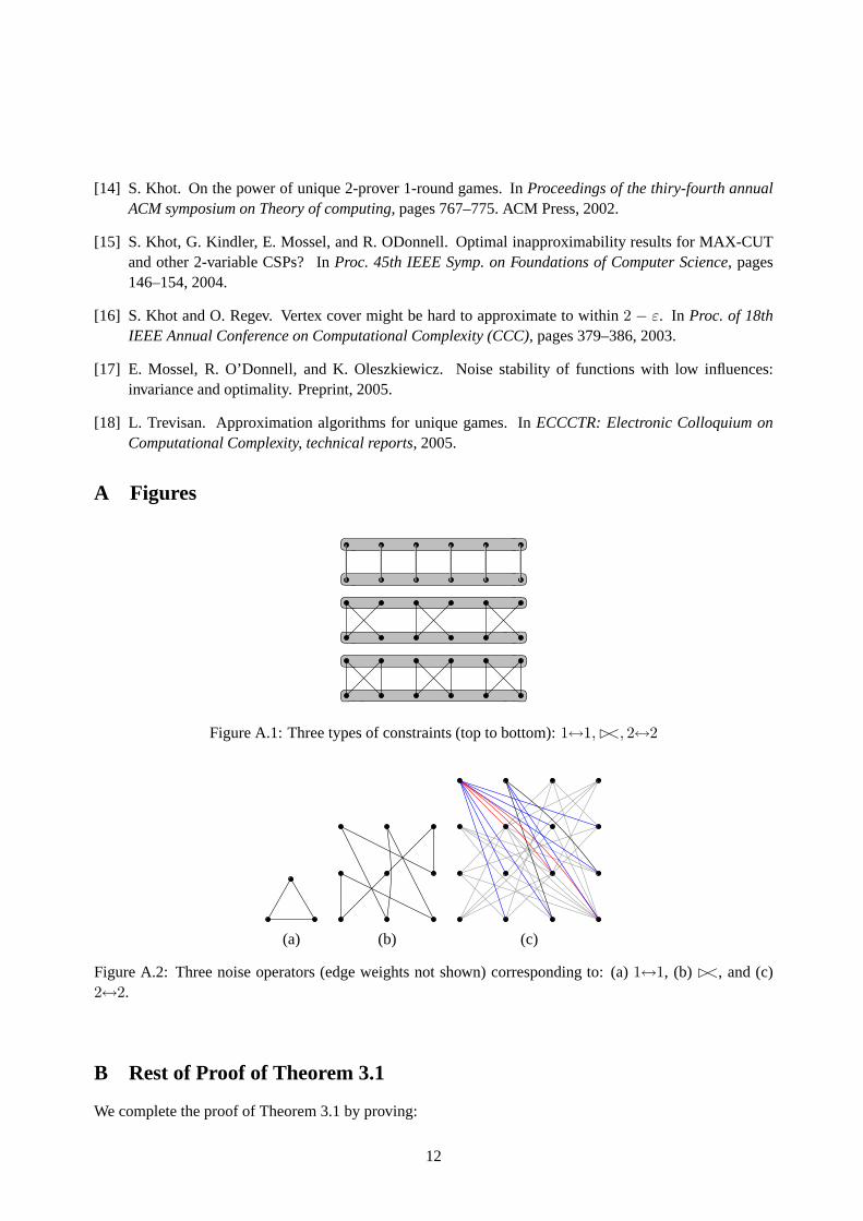
We now consider three conjectures on which our reductions are based. The main difference between thethree conjectures is in the type of constraints that are allowed. The three types are illustrated in Figure A.1.Due to lack of space, we only describe the first conjecture anddefer the remaining two to Appendix C.

Definition 4.3 (1↔1-constraint) A 1↔1 constraint is a relation{(i, π(i))}Ri=1, whereπ : {1, . . . , R} →

{1, . . . , R} is any arbitrary permutation. The constraint is satisfied by(a, b) iff b = π(a).

Conjecture 4.4 (1↔1 Conjecture) For anyε, ζ > 0 andt ∈ N there exists someR ∈ N such that given alabel-cover instanceG = 〈(V,E), R,Ψ〉 where all constraints are1↔1-constraints, it is NP-hard to decidebetween the caseisat(G) ≥ 1 − ζ and the caseisatt(G) < ε.

It is easy to see that the above problem is in P whenζ = 0.

8

4.2 Noise operators

We now define the noise operators corresponding to the1↔1-constraints,⊲<-constraints, and2↔2-constraints.The noise operator that corresponds to the1↔1-constraints is the simplest, and acts on{0, 1, 2}. For theother two cases, since the constraints involve pairs of coordinates, we obtain an operator on{0, 1, 2}2 andan operator on{0, 1, 2, 3}2. See Figure A.2 for an illustration.

Lemma 4.5 There exists a symmetric Markov operatorT on {0, 1, 2} such thatr(T ) < 1 and such that ifT (x↔ y) > 0 thenx 6= y.

Proof: Take the operator given by

T =

0 1/2 1/2

1/2 0 1/2

1/2 1/2 0

.

The two remaining noise operators are described in AppendixD.

4.3 The Reductions

The basic idea in all three reductions is to take a label-cover instance and to replace each vertex with ablock of qR vertices, corresponding to theq-ary hypercube[q]R. The intended way toq-color this blockis by coloringx ∈ [q]R according toxi wherei is the label given to this block. One can think of thiscoloring as an encoding of the labeli. We will essentially prove that any other coloring of this block thatuses relatively few colors, can be “list-decoded” into at most t labels from{1, . . . , R}. By properly definingedges connecting these blocks, we can guarantee that the lists decoded from two blocks can be used ast-labelings for the label-cover instance.

In this section we will describe only the reduction forALMOST-3-COLORING. We defer the two (similar)remaining reductions (forAPPROXIMATE-COLORING(4, Q) and for APPROXIMATE-COLORING(3, Q)) toAppendix E.

In the rest of this section, we use the following notation. For a vectorx = (x1, . . . , xn) and a permutationπ on{1, . . . , n}, we definexπ = (xπ(1), . . . , xπ(n)).

ALMOST -3-COLORING

LetG = ((V,E), R,Ψ) be a label-cover instance as in Conjecture4.4. Forv ∈ V write [v] for a collectionof vertices, one per point in{0, 1, 2}R. Lete = (v, w) ∈ E, and letψ be the1↔1-constraint associated withe. By Definition 4.3 there is a permutationπ such that(a, b) ∈ ψ iff b = π(a). We now write[v, w] for thefollowing collection of edges. We put an edge(x, y) for x = (x1, . . . , xR) ∈ [v] andy = (y1, . . . , yR) ∈ [w]

iff∀i ∈ {1, . . . , R} , T

(

xi ↔ yπ(i)

)

6= 0

whereT is the noise operator from Lemma 4.5. In other words,x is adjacent toy whenever

T⊗R (x↔ yπ) =R

∏

i=1

T(

xi ↔ yπ(i)

)

6= 0.

The reduction outputs the graph[G] = ([V ], [E]) where[V ] is the disjoint union of all blocks[v] and[E] isthe disjoint union of all collections of edges[v, w].

9

Completeness. If isat(G) ≥ 1− ε, then there is someS ⊆ V of size(1− ε) |V | and a labelingℓ : S → R

that satisfies all of the constraints induced byS. We 3-color all of the vertices in∪v∈S [v] as follows.Let c : ∪v∈S [v] → {0, 1, 2} be defined as follows. For everyv ∈ S, the color ofx = (x1, . . . , xR) ∈{0, 1, 2}R = [v] is defined to bec(x):=xi, wherei = ℓ(v) ∈ {1, . . . , R}.

To see thatc is a legal coloring on∪v∈S [v], observe that ifx ∈ [v] andy ∈ [w] share the same color, thenxi = yj for i = ℓ(v) andj = ℓ(w). Sinceℓ satisfies every constraint induced byS, it follows that if (v, w)

is a constraint with an associated permutationπ, thenj = π(i). SinceT (z ↔ z) = 0 for all z ∈ {0, 1, 2},there is no edge betweenx andy.

Soundness. Before presenting the soundness proof, we need the following corollary. It is simply a specialcase of Theorem 3.1 stated in the contrapositive, withε playing the role ofν andµ. Here we use the factthat〈Fε, Uρ(1 − F1−ε)〉γ > 0 wheneverε > 0.

Corollary 4.6 Letq be a fixed integer and letT be a reversible Markov operator on[q] such thatr(T ) < 1.Then for anyε > 0 there existδ > 0 andk ∈ N such that the following holds. For anyf, g : [q]n → [0, 1],if E[f ] ≥ ε, E[g] ≥ ε, and〈f, T⊗ng〉 = 0, then

∃i ∈ {1, . . . , n}, I≤ki (f) ≥ δ and I≤k

i (g) ≥ δ .

We will show that if[G] has an independent setS ⊆ [V ] of relative size≥ 2ε, thenisatt(G) ≥ ε fora fixed constantt > 0 that depends only onε. More explicitly, we will find a setJ ⊆ V , and at-labelingL : J →

(

R≤t

)

such that|J | ≥ ε |V | andL satisfies all the constraints ofG induced byJ . In other words,for every constraintψ over an edge(u, v) ∈ E ∩ J2, there are valuesa ∈ L(u) andb ∈ L(v) such that(a, b) ∈ ψ.

Let J be the set of all verticesv ∈ V such that the fraction of vertices belonging toS in [v] is at leastε.Then, since|S| ≥ 2ε |[V ]|, Markov’s inequality implies|J | ≥ ε |V |.

For eachv ∈ J let fv : {0, 1, 2}R → {0, 1} be the characteristic function of S restricted to[v], soE[fv] ≥ ε. Selectδ, k according to Corollary 4.6 withε and the operatorT of Lemma 4.5, and set

L(v) ={

i ∈ {1, . . . , R}∣

∣

∣ I≤ki (fv) ≥ δ

}

.

Clearly, |L(v)| ≤ k/δ because∑R

i=1 I≤ki (f) ≤ k. Thus,L is a t-labeling fort = k/δ. The main point to

prove is that for every edgee = (v1, v2) ∈ E ∩ J2 induced onJ , there is somea ∈ L(v1) andb ∈ L(v2)

such that(a, b) ∈ ψe. This would imply thatisatt(G) ≥ |J | / |V | ≥ ε.Fix (v1, v2) ∈ E ∩ J2, and letπ be the permutation associated with the1↔1 constraint on this edge.

(It may be easier to first think ofπ = id.) Recall that the edges in[v1, v2] were defined based onπ, andon the noise operatorT defined in Lemma 4.5. Letf = fv1 , and defineg by g(xπ) = fv2(x). SinceS isan independent set,f(x) = fv1(x) = 1 andg(yπ) = fv2(y) = 1 implies thatx, y are not adjacent, so byconstructionT⊗R(x↔ yπ) = 0. Therefore,

〈f, T⊗Rg〉 = 3−R∑

x

f(x)T⊗Rg(x) = 3−R∑

x

f(x)∑

yπ

T⊗R(x↔ yπ)g(yπ) =∑

x,yπ

0 = 0 .

Also, by assumption,E[g] ≥ ε andE[f ] ≥ ε. Corollary 4.6 implies that there is some indexi ∈ {1, . . . , R}for which bothI≤k

i (f) ≥ δ andI≤ki (g) ≥ δ. By definition ofL, i ∈ L(v1). Since thei-th variable ing is

theπ(i)-th variable infv2 , π(i) ∈ L(v2). It follows that there are valuesi ∈ L(v1) andπ(i) ∈ L(v2) suchthat(i, π(i)) satisfies the constraint on(v1, v2). This means thatisatt(G) ≥ |J | / |V | ≥ ε.

10

5 Omitted proofs and discussions

We have omitted from this extended abstract a comparison between the conjectures we have used and Khot’soriginal conjectures. A detailed comparison is given in Appendix G. The rest of the main Fourier theoremis given in Appendix B. The reductions forAPPROXIMATE-COLORINGare given in Appendix E.

Acknowledgements

We thank Uri Zwick for his help with the literature.

References

[1] N. Alon, I. Dinur, E. Friedgut, and B. Sudakov. Graph products, fourier analysis and spectral tech-niques.GAFA, 14(5):913–940, 2004.

[2] M. Bellare, O. Goldreich, and M. Sudan. Free bits, PCPs, and nonapproximability—towards tightresults.SIAM J. Comput., 27(3):804–915, 1998.

[3] A. Blum and D. Karger. AnO(n3/14)-coloring algorithm for3-colorable graphs.Inform. Process.Lett., 61(1):49–53, 1997.

[4] C. Borell. Geometric bounds on the Ornstein-Uhlenbeck velocity process.Z. Wahrsch. Verw. Gebiete,70(1):1–13, 1985.

[5] I. Dinur and S. Safra. On the hardness of approximating minimum vertex cover.Annals of Mathemat-ics, 2005. To appear.

[6] U. Feige and J. Kilian. Zero knowledge and the chromatic number.J. Comput. System Sci., 57(2):187–199, 1998.

[7] M. Furer. Improved hardness results for approximating the chromatic number. InProc. 36th IEEESymp. on Foundations of Computer Science, pages 414–421, 1995.

[8] V. Guruswami and S. Khanna. On the hardness of 4-coloringa 3-colorable graph. In15th AnnualIEEE Conference on Computational Complexity (Florence, 2000), pages 188–197. IEEE ComputerSoc., Los Alamitos, CA, 2000.

[9] E. Halperin, R. Nathaniel, and U. Zwick. Coloringk-colorable graphs using relatively small palettes.J. Algorithms, 45(1):72–90, 2002.

[10] J. Hastad. Some optimal inapproximability results.J. ACM, 48(4):798–859, 2001.

[11] D. Karger, R. Motwani, and M. Sudan. Approximate graph coloring by semidefinite programming.Journal of the ACM, 45(2):246–265, 1998.

[12] S. Khanna, N. Linial, and S. Safra. On the hardness of approximating the chromatic number.Combi-natorica, 20(3):393–415, 2000.

[13] S. Khot. Improved inapproximability results for MaxClique, chromatic number and approximate graphcoloring. InProc. 42nd IEEE Symp. on Foundations of Computer Science, pages 600–609, 2001.

11

[14] S. Khot. On the power of unique 2-prover 1-round games. In Proceedings of the thiry-fourth annualACM symposium on Theory of computing, pages 767–775. ACM Press, 2002.

[15] S. Khot, G. Kindler, E. Mossel, and R. ODonnell. Optimalinapproximability results for MAX-CUTand other 2-variable CSPs? InProc. 45th IEEE Symp. on Foundations of Computer Science, pages146–154, 2004.

[16] S. Khot and O. Regev. Vertex cover might be hard to approximate to within2 − ε. In Proc. of 18thIEEE Annual Conference on Computational Complexity (CCC), pages 379–386, 2003.

[17] E. Mossel, R. O’Donnell, and K. Oleszkiewicz. Noise stability of functions with low influences:invariance and optimality. Preprint, 2005.

[18] L. Trevisan. Approximation algorithms for unique games. In ECCCTR: Electronic Colloquium onComputational Complexity, technical reports, 2005.

A Figures

Figure A.1: Three types of constraints (top to bottom):1↔1,⊲<, 2↔2

(a) (b) (c)

Figure A.2: Three noise operators (edge weights not shown) corresponding to: (a)1↔1, (b) ⊲<, and (c)2↔2.

B Rest of Proof of Theorem 3.1

We complete the proof of Theorem 3.1 by proving:

12

Lemma B.1 Letq be a fixed integer and letT be a symmetric Markov operator on[q] such thatρ = r(T ) <

1. Then for anyε > 0, there exists aδ > 0 and an integerk such that for any functionsf, g : [q]n → [0, 1]

satisfyingE[f ] = µ,E[g] = ν and

∀i min(

I≤ki (f), I≤k

i (g))

< δ (3)

then〈f, T⊗ng〉 ≤ 〈Fµ, UρFν〉γ + ε. (4)

Proof: Let f1 = T⊗nη f andg1 = T⊗n

η g whereη < 1 is chosen so thatρj(1 − η2j) < ε/4 for all j. Then

|〈f1, T⊗ng1〉 − 〈f, T⊗ng〉| =

∣

∣

∣

∑

x

f(αx)g(αx)∏

a 6=0

λ|x|aa (1 − η2|x|)∣

∣

∣

≤∑

x

ρ|x|(1 − η2|x|)∣

∣

∣f(αx)g(αx)∣

∣

∣ ≤ ε/4

where the last inequality follows from the Cauchy-Schwartzinequality. Thus, in order to prove (4) it sufficesto prove

〈f1, T⊗ng1〉 ≤ 〈Fµ, UρFν〉γ + 3ε/4. (5)

Let δ(ε/4, η) be the value given by Lemma 3.9 plugging inε/4 for ε. Let δ′ = δ(ε/4, η)/2. Let k bechosen so thatη2k < min(δ′, ε/4). DefineC = k/δ′ andδ = (ε/8C)2 < δ′ . Let

Bf = {i : I≤ki (f) ≥ δ′}, Bg = {i : I≤k

i (g) ≥ δ′}.

We note thatBf andBg are of size at mostC = k/δ′. By (3), we have that wheneveri ∈ Bf , I≤ki (g) < δ.

Similarly, for everyi ∈ Bg we haveI≤ki (f) < δ. In particular,Bf andBg are disjoint.

Recall the averaging operatorA. We now let

f2(x) = ABf(f1) =

∑

x:xBf=0

f(αx)αxη|x|,

g2(x) = ABg (g1) =∑

x:xBg =0

g(αx)αxη|x|.

Clearly, E[f2] = E[f ] and E[g2] = E[g], and for allx f2(x), g2(x) ∈ [0, 1]. It is easy to see thatIi(f2) = 0 if i ∈ Bf andIi(f2) ≤ I≤k

i (f) + η2k < 2δ′ otherwise and similarly forg2. Thus, for anyi, max (Ii(f2), Ii(g2)) < 2δ′. We also see that for anyx, |f2(αx)| ≤ η|x| and the same forg2. Thus, we canapply Lemma 3.9 to obtain that

〈f2, T⊗ng2〉 ≤ 〈Fµ, UρFν〉γ + ε/4.

In order to show (5) and complete the proof, we show that

|〈f1, T⊗ng1〉 − 〈f2, T

⊗ng2〉| ≤ ε/2.

13

This follows by

|〈f1, T⊗ng1〉 − 〈f2, T

⊗ng2〉| =∣

∣

∣

∑

x:xBf ∪Bg 6=0

f(αx)g(αx)∏

a 6=0

λ|x|aa η2|x|∣

∣

∣

≤ η2k∑

x:|x|≥k

∣

∣

∣f(αx)g(αx)∣

∣

∣ +∑

{∣

∣

∣f(αx)g(αx)∣

∣

∣ : xBf∪Bg 6= 0, |x| ≤ k}

≤ ε/4 +∑

i∈Bf∪Bg

∑

{∣

∣

∣f(αx)g(αx)∣

∣

∣ : xi 6= 0, |x| ≤ k}

≤ ε/4 +∑

i∈Bf∪Bg

√

I≤ki (f)

√

I≤ki (g)

≤ ε/4 +√δ(|Bf | + |Bg|)

≤ ε/4 + 2C√δ = ε/2,

where the next-to-last inequality holds because for eachi ∈ Bf ∪ Bg one ofI≤ki (f), I≤k

i (g) is at mostδand the other is at most1.

The final theorem of this section is needed only for theAPPROXIMATE-COLORING(3, Q) result. Here,the operatorT acts on[q2] and is assumed to have an additional property. Before proceeding, it is helpful torecall Definition 2.6.

Theorem B.2 Let q be a fixed integer and letT be a symmetric Markov operator on[q2] such thatρ =

r(T ) < 1. Suppose moreover, thatT has the following property. Given(x1, x2) chosen uniformly atrandom and(y1, y2) chosen according toT applied to(x1, x2) we have that(x2, y2) is distributed uniformlyat random. Then for anyε > 0, there exists aδ > 0 and an integerk such that for any functionsf, g :

[q]2n → [0, 1] satisfyingE[f ] = µ,E[g] = ν, and fori = 1, . . . , n

min(

I≤k2i−1(f), I≤k

2i−1(g))

< δ, min(

I≤k2i−1(f), I≤k

2i (g))

< δ, and min(

I≤k2i (f), I≤k

2i−1(g))

< δ

it holds that〈f, T⊗ng〉 ≥ 〈Fµ, Uρ(1 − F1−ν)〉γ − ε (6)

and〈f, T⊗ng〉 ≤ 〈Fµ, UρFν〉γ + ε. (7)

Proof: As in Theorem 3.1, (6) follows from (7) so it is enough to prove(7). Assume first that in addition tothe three conditions above we also have that for alli = 1, . . . , n,

min(

I≤k2i (f), I≤k

2i (g))

< δ. (8)

Then it follows that for alli, either bothI≤k2i−1(f) andI≤k

2i (f) are smaller thanδ or bothI≤k2i−1(g) andI≤k

2i (g)

are smaller thanδ. Hence, by Claim 2.7, we know that for alli we have

min(

I≤k/2i (f), I

≤k/2i (g)

)

< 2δ

and the result then follows from Lemma B.1. However, we do nothave this extra condition and hence wehave to deal with ‘bad’ coordinatesi for whichmin(I≤k

2i (f), I≤k2i (g)) ≥ δ. Notice for suchi it must be the

case that bothI≤k2i−1(f) andI≤k

2i−1(g) are smaller thanδ. Informally, the proof proceeds as follows. We first

14

define functionsf1, g1 that are obtained fromf, g by adding a small amount of noise. We then obtainf2, g2from f1, g1 by averaging the coordinates2i− 1 for badi. Finally, we obtainf3, g3 from f2, g2 by averagingthe coordinate2i for bad i. The point here is to maintain〈f, T⊗ng〉 ≈ 〈f1, T

⊗ng1〉 ≈ 〈f2, T⊗ng2〉 ≈

〈f3, T⊗ng3〉. The condition in Equation 8 now applies tof3, g3 and we can apply Lemma B.1, as described

above. We now describe the proof in more detail.We first definef1 = T⊗n

η f andg1 = T⊗nη g whereη < 1 is chosen so thatρj(1 − η2j) < ε/4 for all j.

As in the previous lemma it is easy to see that

|〈f1, T⊗ng1〉 − 〈f, T⊗ng〉| < ε/4

and thus it suffices to prove that

〈f1, T⊗ng1〉 ≤ 〈Fµ, UρFν〉γ + 3ε/4.

Let δ(ε/2, η), k(ε/2, η) be the values given by Lemma B.1 withε taken to beε/2. Letδ′ = δ(ε/2, η)/2.Choose a large enoughk so that128kηk < ε2δ′ andk/2 > k(ε/2, η). We letC = k/δ′ andδ = ε2/128C.Notice thatδ < δ′ andηk < δ. Finally, let

B ={

i∣

∣

∣ I≤k2i (f) ≥ δ′, I≤k

2i (g) ≥ δ′}

.

We note thatB is of size at mostC. We also note that ifi ∈ B then we haveI≤k2i−1(f) < δ andI≤k

2i−1(g) < δ.We claim that this implies thatI2i−1(f1) ≤ δ+ηk < 2δ and similarly forg. To see that, take any orthonormalbasisβ0 = 1, β1, . . . , βq−1 of R

q and notice that we can write

f1 =∑

x∈[q]2n

f(βx)η|x|βx.

Hence,I2i−1(f1) =

∑

x ∈ [q]2n

x2i−1 6= 0

f(βx)2η2|x| < δ + ηk∑

x ∈ [q]2n

|x| > k

f(βx)2 ≤ δ + ηk

where we used that the number of nonzero elements inx is at least half of that inx.Next, we definef2 = A2B−1(f1) andg2 = A2B−1(g1) whereA is the averaging operator and2B − 1

denotes the set{2i− 1 | i ∈ B}. Note that

‖f2 − f1‖22 = ‖f2 − f1‖2

2 ≤∑

i∈B

I2i−1(f1) ≤ 2Cδ.

and similarly,‖g2 − g1‖2

2 = ‖g2 − g1‖22 ≤ 2Cδ.

Thus

|〈f1, T⊗ng1〉 − 〈f2, T

⊗ng2〉| ≤ |〈f1, T⊗ng1〉 − 〈f1, T

⊗ng2〉| + |〈f1, T⊗ng2〉 − 〈f2, T

⊗ng2〉|≤ 2

√2Cδ = ε/4

where the last inequality follows from the Cauchy-Schwartzinequality together with the fact that‖f1‖2 ≤ 1

and also‖T⊗ng2‖2 ≤ 1. Hence, it suffices to prove

〈f2, T⊗ng2〉 ≤ 〈Fµ, UρFν〉γ + ε/2.

15

We now definef3 = A2B(f2) andg3 = A2B(g2). Equivalently, we havef3 = AB(f1) andg3 =

AB(g1). We show that〈f2, T⊗ng2〉 = 〈f3, T

⊗ng3〉. Let αx, x ∈ [q2]n, be an orthonormal basis of eigen-vectors ofT⊗n. Then

〈f3, T⊗ng3〉 =

∑

x,y∈[q2]n,xB=yB=0

f1(αx)g1(αy)〈αx, T⊗nαy〉.

Moreover, sinceA is a linear operator andf1 can be written as∑

x∈[q2]n f1(αx)αx and similarly forg1, wehave

〈f2, T⊗ng2〉 =

∑

x,y∈[q2]n

f1(αx)g1(αy)〈A2B−1(αx), T⊗nA2B−1(αy)〉.

First, notice that whenxB = 0,A2B−1(αx) = αx sinceαx does not depend on coordinates inB. Hence, inorder to show that the two expressions above are equal, it suffices to show that

〈A2B−1(αx), T⊗nA2B−1(αy)〉 = 0

unlessxB = yB = 0. So assume without loss of generality thati ∈ B is such thatxi 6= 0. The above innerproduct can be equivalently written as

Ez,z′∈[q2]n [A2B−1(αx)(z) ·A2B−1(αy)(z′)]

wherez is chosen uniformly at random andz′ is chosen according toT⊗n applied toz. Fix some arbitraryvalues toz1, . . . , zi−1, zi+1, . . . , zn andz′1, . . . , z

′i−1, z

′i+1, . . . , z

′n and let us show that

Ezi,z′i∈[q2][A2B−1(αx)(z) ·A2B−1(αy)(z′)] = 0.

Sincei ∈ B, the two expressions inside the expectation do not depend onzi,1 andz′i,1 (where byzi,1 wemean the first coordinate ofzi). Moreover, by our assumption onT , zi,2 andz′i,2 are independent. Hence,the above expectation is equal to

Ezi∈[q2][A2B−1(αx)(z)] · Ez′i∈[q2][A2B−1(αy)(z′)].

Sincexi 6= 0, the first expectation is zero. This establishes that〈f2, T⊗ng2〉 = 〈f3, T

⊗ng3〉.The functionsf3, g3 satisfy the property that for everyi = 1, . . . , n, either bothI≤k

2i−1(f3) andI≤k2i (f3)

are smaller thanδ′ or bothI≤k2i−1(g3) andI≤k

2i (g3) are smaller thanδ′. By Claim 2.7, we get that fori =

1, . . . , n, eitherI≤k/2i (f3) or I≤k/2

i (g3) is smaller2δ′. We can now apply Lemma B.1 to obtain

〈f3, T⊗ng3〉 ≤ 〈Fµ, UρFν〉γ + ε/2.

C The Two Remaining Conjectures

Definition C.1 (2↔2-constraint) A2↔2 constraint is defined by a pair of permutationsπ1, π2 : {1, . . . , 2R} →{1, . . . , 2R} and the relation

2↔2 = {(2i, 2i), (2i, 2i− 1), (2i− 1, 2i), (2i− 1, 2i− 1)}Ri=1 .

The constraint is satisfied by(a, b) iff (π−11 (a), π−1

2 (b)) ∈ 2↔2.

16

Definition C.2 (⊲<-constraint) An⊲< constraint is defined by a pair of permutationsπ1, π2 : {1, . . . , 2R} →{1, . . . , 2R} and the relation

⊲< = {(2i− 1, 2i− 1), (2i, 2i− 1), (2i− 1, 2i)}Ri=1 .

The constraint is satisfied by(a, b) iff (π−11 (a), π−1

2 (b)) ∈ ⊲<.

Conjecture C.3 (2↔2 Conjecture) For any ε > 0 and t ∈ N there exists someR ∈ N such that givena label-cover instanceG = 〈(V,E), 2R,Ψ〉 where all constraints are2↔2-constraints, it is NP-hard todecide between the casesat(G) = 1 and the caseisatt(G) < ε.

The 1↔1 conjecture and the above conjecture are no stronger than thecorresponding conjectures ofKhot. Namely, our1↔1 conjecture is not stronger than Khot’s (bipartite) unique games conjecture, andour 2↔2 conjecture is not stronger than Khot’s (bipartite)2→1 conjecture. The former claim was al-ready proven by Khot and Regev in [16]. The latter claim is proven in a similar way. For completeness,we include both proofs in Appendix G. We also make a third conjecture that is used in our reduction toAPPROXIMATE-COLORING(3, Q). This conjecture seems stronger than Khot’s conjectures.

Conjecture C.4 (⊲< Conjecture) For any ε > 0 and t ∈ N there exists someR ∈ N such that given alabel-cover instanceG = 〈(V,E), 2R,Ψ〉 where all constraints are⊲<-constraints, it is NP-hard to decidebetween the casesat(G) = 1 and the caseisatt(G) < ε.

Remark: The (strange-looking)⊲<-shaped constraints have already appeared before, in [5]. There, it is (im-plicitly) proven that for allε, ζ > 0 given a label-cover instanceG where all constraints are⊲<-constraints,it is NP-hard to distinguish between the caseisat(G) > 1 − ζ and the caseisatt=1(G) < ε. The maindifference between their case and our conjecture is that in our conjecture we consider any constantt, whilein their caset is 1.

D The Two Remaining Operators

Lemma D.1 There exists a symmetric Markov operatorT on{0, 1, 2, 3}2 such thatr(T ) < 1 and such thatif T ((x1, x2) ↔ (y1, y2)) > 0 then{x1, x2} ∩ {y1, y2} = ∅.

Proof: Our operator has three types of transitions, with transitions probabilitiesβ1, β2, andβ3.

• With probabilityβ1 we have(x, x) ↔ (y, y) wherex 6= y.

• With probabilityβ2 we have(x, x) ↔ (y, z) wherex, y, z are all different.

• With probabilityβ3 we have(x, y) ↔ (z, w) wherex, y, z, w are all different.

These transitions are illustrated in Figure A.2(c) with redindicatingβ1 transitions, blue indicatingβ2 transi-tions, and black indicatingβ3 transitions. ForT to be symmetric Markov operator, we need thatβ1, β2 andβ3 are non-negative and

3β1 + 6β2 = 1, 2β2 + 2β3 = 1.

It is easy to see that the two equations above have solutions bounded away from0 and that the correspondingoperator hasr(T ) < 1. For example, chooseβ1 = 1/12, β2 = 1/8, andβ3 = 3/8.

17

Lemma D.2 There exists a symmetric Markov operatorT on{0, 1, 2}2 such thatr(T ) < 1 and such that ifT ((x1, x2) ↔ (y1, y2)) > 0 thenx1 /∈ {y1, y2} andy1 /∈ {x1, x2}. Moreover, the noise operatorT satisfiesthe following property. Let(x1, x2) be chosen according to the uniform distribution and(y1, y2) be chosenaccordingT applied to(x1, x2). Then the distribution of(x2, y2) is uniform.

Proof: The proof resembles the previous proof. Again there are3 types of transitions.

• With probabilityβ1 we have(x, x) ↔ (y, y) wherex 6= y.

• With probabilityβ2 we have(x, x) ↔ (y, z) wherex, y, z are all different.

• With probabilityβ3 we have(x, y) ↔ (z, y) wherex, y, z are all different.

ForT to be a symmetric Markov operator we requireβ1, β2 andβ3 to be non-negative and

2β1 + 2β2 = 1, β2 + β3 = 1.

Moreover, the last requirement of uniformity of(x2, y2) amounts to the equation

β1/3 + 2β2/3 = 2β3/3.

It is easy to see thatβ2 = β3 = 0.5 andβ1 = 0 is the solution of all equations and that the correspondingoperator hasr(T ) < 1. This operator is illustrated in Figure A.2(b).

E The Two Remaining Reductions

The basic idea in all three reductions is to take a label-cover instance and to replace each vertex with ablock of qR vertices, corresponding to theq-ary hypercube[q]R. The intended way toq-color this blockis by coloringx ∈ [q]R according toxi wherei is the label given to this block. One can think of thiscoloring as an encoding of the labeli. We will essentially prove that any other coloring of this block thatuses relatively few colors, can be “list-decoded” into at most t labels from{1, . . . , R}. By properly definingedges connecting these blocks, we can guarantee that the lists decoded from two blocks can be used ast-labelings for the label-cover instance.

In the rest of this section, we use the following notation. For a vectorx = (x1, . . . , xn) and a permutationπ on{1, . . . , n}, we definexπ = (xπ(1), . . . , xπ(n)).

APPROXIMATE -COLORING (4, Q): This reduction is nearly identical to the one above, with thefollowingchanges:

• The starting point of the reduction is an instanceG = ((V,E), 2R,Ψ) as in Conjecture C.3.

• Each vertexv is replaced by a copy of{0, 1, 2, 3}2R (which we still denote[v]).

• For every(v, w) ∈ E, let ψ be the2↔2-constraint associated withe. By Definition C.1 there aretwo permutationsπ1, π2 such that(a, b) ∈ ψ iff (π−1

1 (a), π−12 (b)) ∈ 2↔2. We now write[v, w]

for the following collection of edges. We put an edge(x, y) for x = (x1, . . . , x2R) ∈ [v] andy =

(y1, . . . , y2R) ∈ [w] if

∀i ∈ {1, . . . , R} , T ((xπ1(2i−1), xπ1(2i)) ↔ (yπ2(2i−1), yπ2(2i))) 6= 0

whereT is the noise operator from Lemma D.1. Equivalently, we put anedge ifT⊗R(xπ1 ↔ yπ2) 6=0.

As before, the reduction outputs the graph[G] = ([V ], [E]) where[V ] is the union of all blocks[v] and[E]

is the union of collection of the edges[v, w].

18

APPROXIMATE -COLORING (3, Q): Here again the reduction is nearly identical to the above, with thefollowing changes:

• The starting point of the reduction is an instance of label-cover, as in Conjecture C.4.

• Each vertexv is replaced by a copy of{0, 1, 2}2R (which we again denote[v]).

• For every(v, w) ∈ E, let π1, π2 be the permutations associated with the constraint, as in Defini-tion C.2. Define a collection[v, w] of edges, by including the edge(x, y) ∈ [v] × [w] iff

∀i ∈ {1, . . . , R} , T ((xπ1(2i−1), xπ1(2i)) ↔ (yπ2(2i−1), yπ2(2i))) 6= 0

whereT is the noise operator from Lemma D.2. As before, this condition can be written asT⊗R(xπ1 ↔yπ2) 6= 0.

As before, we look at the coloring problem of the graph[G] = ([V ], [E]) where[V ] is the union of all blocks[v] and[E] is the union of collection of the edges[v, w].

E.1 Completeness

APPROXIMATE -COLORING (4, Q): Let ℓ : V → {1, . . . , 2R} be a labeling that satisfies all the con-straints inG. We define a legal4-coloringc : [V ] → {0, 1, 2, 3} as follows. For a vertexx = (x1, . . . , x2R) ∈{0, 1, 2, 3}2R = [v] setc(x):=xi, wherei = ℓ(v) ∈ {1, . . . , 2R}.

To see thatc is a legal coloring, fix any2↔2 constraint(v, w) ∈ E and letπ1, π2 be the permutationsassociated with it. Leti = ℓ(v) andj = ℓ(w), so by assumption(π−1

1 (i), π−12 (j)) ∈ 2↔2. In other words

there is somek ∈ {1, . . . , R} such thati ∈ {π1(2k − 1), π1(2k)} andj ∈ {π2(2k − 1), π2(2k)}. If x ∈ [v]

andy ∈ [w] share the same color, thenxi = c(x) = c(y) = yj . Since

xi ∈{

xπ12k−1, x

π12k

}

and yj ∈{

yπ22k−1, y

π22k

}

we have that the above sets intersect. This, by Lemma D.1, implies thatT⊗R(xπ1 ↔ yπ2) = 0. So theverticesx, y cannot be adjacent, hence the coloring is legal.

APPROXIMATE -COLORING (3, Q): Here the argument is nearly identical to the above. Letℓ : V →{1, . . . , 2R} be a labeling that satisfies all of the constraints inG. We define a legal3-coloringc : [V ] →{0, 1, 2} like before: c(x):=xi, wherei = ℓ(v) ∈ {1, . . . , 2R}. To see thatc is a legal coloring, fix anyedge(v, w) ∈ E and letπ1, π2 be the permutations associated with the⊲<-constraint. Leti = ℓ(v) andj = ℓ(w), so by assumption(π−1

1 (i), π−12 (j)) ∈ ⊲<. In other words there is somek ∈ {1, . . . , R} such

that i ∈ {π1(2k − 1), π1(2k)} andj ∈ {π2(2k − 1), π2(2k)} and not bothi = π1(2k) andj = π2(2k).Assume, without loss of generality, thati = π1(2k − 1), soxi = xπ1

2k−1 andyj ∈{

yπ22k−1, y

π22k

}

.If x ∈ [v] andy ∈ [w] share the same color, thenxi = c(x) = c(y) = yj , so

xπ12k−1 = xi = yj ∈

{

yπ22k−1, y

π22k

}

.

By Lemma D.2 this impliesT ((xπ12k−1, x

π12k) ↔ (yπ2

2k−1, yπ22k)) = 0, which means there is no edge betweenx

andy.

19

E.2 Soundness

APPROXIMATE -COLORING (4, Q): We outline the argument and emphasize only the modifications. As-sume that[G] contains an independent setS ⊆ [V ] whose relative size is at least1/Q and setε = 1/2Q.

• Let fv : {0, 1, 2, 3}2R → {0, 1} be the characteristic function ofS in [v]. Define the setJ ⊆ V asbefore and for allv ∈ J , define

L(v) =

{

i ∈ {1, . . . , 2R}∣

∣

∣

∣

I≤2ki (fv) ≥

δ

2

}

wherek, δ are the values given by Corollary 4.6 withε and the operatorT of Lemma D.1. Asbefore,|J | ≥ ε |V | andE[fv] ≥ ε for v ∈ J . Now L is a t-labeling witht = 4k/δ. Fix an edge(v, w) ∈ E ∩ J2 and letπ1, π2 be the associated permutations. Definef, g by f(xπ1):=fv1(x) andg(yπ2):=fv2(y).

• SinceS is an independent set,f(xπ1) = fv1(x) = 1 andg(yπ2) = fv2(y) = 1 implies thatx, y arenot adjacent, so by constructionT (xπ1 ↔ yπ2) = 0. Therefore,〈f, Tg〉 = 0.

• Now, recalling Definition 2.6, consider the functionsf, g : ({0, 1, 2, 3}2)R → {0, 1}. ApplyingCorollary 4.6 onf, g we may deduce the existence of an indexi ∈ {1, . . . , R} for which bothI≤ki (f) ≥ δ and I≤k

i (g) ≥ δ. By Claim 2.7, δ ≤ I≤ki (f) ≤ I≤2k

2i−1(f) + I≤2k2i (f), so either

I≤2k2i−1(f) ≥ δ/2 or I≤2k

2i (f) ≥ δ/2. Since thej-th variable inf is theπ1(j)-th variable infv1 ,this puts eitherπ1(2i) or π1(2i − 1) in L(v1). Similarly, at least one ofπ2(2i), π2(2i − 1) is inL(v2). Thus, there area ∈ L(v1) andb ∈ L(v2) such that(π−1

1 (a), π−12 (b)) ∈ 2↔2 soL satisfies the

constraint on(v1, v2).

We have shown thatL satisfies every constraint induced byJ , soisatt(G) ≥ ε.

APPROXIMATE -COLORING (3, Q): The argument here is similar to the previous one. The main differenceis in the third step, where we replace Corollary 4.6 by the following corollary of Theorem B.2. The corollaryfollows by lettingε play the role ofµ andν, and using the fact that〈Fε, Uρ(1 − F1−ε)〉γ > 0 wheneverε > 0.

Corollary E.1 Let T be the operator on{0, 1, 2}2 defined in Lemma D.2. For anyε > 0, there existsδ > 0, k ∈ N, such that for any functionsf, g : {0, 1, 2}2R → [0, 1] satisfyingE[f ] ≥ ε,E[g] ≥ ε, thereexists somei ∈ {1, . . . , R} such that either

min(

I≤k2i−1(f), I≤k

2i−1(g))

≥ δ or min(

I≤k2i−1(f), I≤k

2i (g))

≥ δ or min(

I≤k2i (f), I≤k

2i−1(g))

≥ δ.

Now we have functionsfv : {0, 1, 2}2R → {0, 1}, andJ is defined as before. Define a labeling

L(v) ={

i ∈ {1, . . . , 2R}∣

∣

∣ I≤ki (fv) ≥ δ

}

wherek, δ are the values given by Corollary E.1 withε. ThenL is at-labeling witht = k/δ.Let us now show thatL is a satisfyingt-labeling. Let(v1, v2) be a⊲<-constraint with associated

permutationsπ1, π2. Definef(xπ1) = fv1(x), g(xπ2) = fv2(x). We apply Corollary E.1 onf, g, and obtain

an indexi ∈ {1, . . . , R}. Since thej-th variable inf is theπ1(j)-th variable infv1 , this puts eitherπ1(2i)

orπ1(2i−1) in L(v1). Similarly, at least one ofπ2(2i), π2(2i−1) is inL(v2). Moreover, we are guaranteedthat eitherπ1(2i− 1) ∈ L(v1) or π2(2i − 1) ∈ L(v2). Thus, there area ∈ L(v1) andb ∈ L(v2) such that(π−1

1 (a), π−12 (b)) ∈ ⊲< soL satisfies the constraint on(v1, v2).

20

F Omitted Proofs

F.1 Proof of Claim 2.4

Let us first fix the values ofx1, . . . , xi−1, xi+1, . . . , xn. Then

Vxi[f ] = Vxi

[

∑

y

f(αy)αy

]

= Vxi

[

∑

y:yi 6=0

f(αy)αy

]

,

where the last equality follows from the fact that ifyi = 0 thenαy is a constant function ofxi. If yi 6= 0,then the expected value ofαy with respect toxi is zero. Therefore,

Vxi

[

∑

y:yi 6=0

f(αy)αy

]

= Exi

∑

y:yi 6=0

f(αy)αy

2

= Exi

∑

y,z:yi 6=0,zi 6=0

f(αy)f(αz)αyαz

.

Thus,

Ii(f) = Ex

∑

y,z:yi 6=0,zi 6=0

f(αy)f(αz)αyαz

=∑

y,z:yi 6=0,zi 6=0

f(αy)f(αz)Ex[αyαz] =∑

y:yi 6=0

f2(αy),

as needed.

G Comparison with Khot’s Conjectures

Let us first state Khot’s original conjectures. Ford ≥ 1, an instance of the weighted bipartited-to-1 labelcover problem is given by a tupleΦ = (X,Y,Ψ,W ). We often refer to vertices inX asleft vertices and tovertices inY asright vertices. The setΨ consists of oned-to-1 relationψxy for eachx ∈ X andy ∈ Y .More precisely,ψxy ⊆ {1, . . . , R}×{1, . . . , R/d} is such that for anyb ∈ {1, . . . , R/d} there are preciselyd elementsa ∈ {1, . . . , R} such that(a, b) ∈ ψxy. The setW includes a non-negative weightwxy ≥ 0

for eachx ∈ X, y ∈ Y . We denote byw(Φ, x) the sum∑

y∈Y wxy and byw(Φ) the sum∑

x∈X,y∈Y wxy.A labeling is a functionL mappingX to {1, . . . , R} andY to {1, . . . , R/d}. A constraintψxy is satisfiedby a labelingL if (L(x), L(y)) ∈ ψxy. Also, for a labelingL, the weight of satisfied constraints, denotedby wL(Φ), is

∑

wxy where the sum is taken over allx ∈ X andy ∈ Y such thatψxy is satisfied byL.Similarly, we definewL(Φ, x) as

∑

wxy where the sum is now taken over ally ∈ Y such thatψxy is satisfiedbyL. The following conjectures were presented in [14].

Conjecture G.1 (Bipartite 1-to-1 Conjecture) For any ζ, γ > 0 there exists a constantR such that thefollowing is NP-hard. Given a1-to-1 label cover instanceΦ with label set{1, . . . , R} andw(Φ) = 1

distinguish between the case where there exists a labelingL such thatwL(Φ) ≥ 1 − ζ and the case wherefor any labelingL, wL(Φ) ≤ γ.

In the following conjecture,d is any fixed integer greater than1.

Conjecture G.2 (Bipartite d-to-1 Conjecture) For anyγ > 0 there exists a constantR such that the fol-lowing is NP-hard. Given a bipartited-to-1 label cover instanceΦ with label sets{1, . . . , R}, {1, . . . , R/d}andw(Φ) = 1 distinguish between the case where there exists a labelingL such thatwL(Φ) = 1 and thecase where for any labelingL, wL(Φ) ≤ γ.

21

The theorem we prove in this section is the following.

Theorem G.3 Conjecture 4.4 follows from Conjecture G.1 and Conjecture C.3 follows from Conjecture G.2for d = 2.1

The proof follows by combining Lemmas G.4, G.5, G.7, and G.9.Each lemma presents an elementarytransformation between variants of the label cover problem. The first transformation modifies a bipartitelabel cover instance so that allX variables have the same weight. When we say below thatΦ′ has the sametype of constraints asΦ we mean that the transformation only duplicates existing constraints and hence ifΦconsists ofd-to-1 constraints for somed ≥ 1, then so doesΦ′.

Lemma G.4 There exists an efficient procedure that given a weighted bipartite label cover instanceΦ =

(X,Y,Ψ,W ) with w(Φ) = 1 and a constantℓ, outputs a weighted bipartite label cover instanceΦ′ =

(X ′, Y,Ψ′,W ′) on the same label sets and with the same type of constraints with the following properties:

• For all x ∈ X ′, w(Φ′, x) = 1.

• For anyζ ≥ 0, if there exists a labelingL to Φ such thatwL(Φ) ≥ 1−ζ then there exists a labelingL′

to Φ′ in which1−√

(1 + 1ℓ−1)ζ of the variablesx inX ′ satisfy thatwL′(Φ′, x) ≥ 1−

√

(1 + 1ℓ−1)ζ.

In particular, if there exists a labelingL such thatwL(Φ) = 1 then there exists a labelingL′ in whichall variables satisfywL′(Φ′, x) = 1.

• For any β2, γ > 0, if there exists a labelingL′ to Φ′ in which β2 of the variablesx in X ′ satisfywL′(Φ′, x) ≥ γ, then there exists a labelingL to Φ such thatwL(Φ) ≥ (1 − 1

ℓ )β2γ.

Proof: GivenΦ as above, we defineΦ′ = (X ′, Y,Ψ′,W ′) as follows. The setX ′ includesk(x) copies ofeachx ∈ X, x(1), . . . , x(k(x)) wherek(x) is defined as⌊ℓ · |X| · w(Φ, x)⌋. For everyx ∈ X, y ∈ Y andi ∈ {1, . . . , k(x)} we defineψ′

x(i)yasψxy and the weightw′

x(i)yaswxy/w(Φ, x). Notice thatw(Φ′, x) = 1

for all x ∈ X ′ and that(ℓ − 1)|X| ≤ |X ′| ≤ ℓ|X|. Moreover, for anyx ∈ X, y ∈ Y , the total weight ofconstraints created fromψxy is k(x)wxy/w(Φ, x) ≤ ℓ|X|wxy.

We now prove the second property. Given a labelingL to Φ that satisfies constraints of weight at least1 − ζ, consider the labelingL′ defined byL′(x(i)) = L(x) andL′(y) = L(y). By the property mentionedabove, the total weight of unsatisfied constraints inΦ′ is at mostℓ|X|ζ. Since the total weight inΦ′ is at least(ℓ− 1)|X|, we obtain that the fraction of unsatisfied constraints is atmost(1 + 1

ℓ−1)ζ. Hence, by a Markov

argument, we obtain that for at least1−√

(1 + 1ℓ−1)ζ of theX ′ variableswL′(Φ′, x) ≥ 1−

√

(1 + 1ℓ−1)ζ.

We now prove the third property. Assume we are given a labelingL′ to Φ′ for whichβ2 of the variableshavewL′(Φ′, x) ≥ γ. Without loss of generality we can assume that for everyx ∈ X, the labelingL′(x(i))

is the same for alli. This holds since the constraints betweenx(i) and theY variables are the same for alli ∈ {1, . . . , k(x)}. We define the labelingL asL(x) = L′(x(1)). The weight of constraints satisfied byLis:

∑

x∈X

wL(Φ, x) ≥ 1

ℓ|X|∑

x∈X

k(x) · wL(Φ, x)/w(Φ, x)

=1

ℓ|X|∑

x∈X′

wL′(Φ′, x)

≥ 1

ℓ|X|β2|X ′|γ ≥(

1 − 1

ℓ

)

β2γ

1We in fact show that for anyd ≥ 2, the natural extension of Conjecture C.3 tod-to-d constraints follows from Conjecture G.2with the same value ofd.

22

where the first inequality follows from the definition ofk(x).

The second transformation creates anunweightedlabel cover instance. Such an instance is given by atuple Φ = (X,Y,Ψ, E). The multisetE includes pairs(x, y) ∈ X × Y and we can think of(X,Y,E)

as a bipartite graph (possibly with parallel edges). For each e ∈ E, Ψ includes a constraint, as before.The instances created by this transformation are left-regular, in the sense that the number of constraints(x, y) ∈ E incident to eachx ∈ X is the same.

Lemma G.5 There exists an efficient procedure that given a weighted bipartite label cover instanceΦ =

(X,Y,Ψ,W ) withw(Φ, x) = 1 for all x ∈ X and a constantℓ, outputs an unweighted bipartite label coverinstanceΦ′ = (X,Y,Ψ′, E′) on the same label sets and with the same type of constraints with the followingproperties:

• All left degrees are equal toα = ℓ|Y |.

• For anyβ, ζ > 0, if there exists a labelingL to Φ such thatwL(Φ, x) ≥ 1 − ζ for at least1 − β ofthe variables inX, then there exists a labelingL′ to Φ′ in which for at least1 − β of the variables inX, at least1 − ζ − 1/ℓ of their incident constraints are satisfied. Moreover, if there exists a labelingL such thatwL(Φ, x) = 1 for all x then there exists a labelingL′ to Φ′ that satisfies all constraints.

• For anyβ, γ > 0, if there exists a labelingL′ to Φ′ in whichβ of the variables inX haveγ of theirincident constraints satisfied, then there exists a labelingL to Φ such that forβ of the variables inX,wL(Φ, x) > γ − 1/ℓ.

Proof: We define the instanceΦ′ = (X,Y,Ψ′, E′) as follows. For eachx ∈ X, choose somey0(x) ∈ Y

such thatwxy0(x) > 0. For everyx ∈ X, y 6= y0(x), E′ contains⌊αwxy⌋ edges fromx to y associatedwith the constraintψxy. Moreover, for everyx ∈ X,E′ containsα−∑

y∈Y \{y0(x)}⌊αwxy⌋ edges fromx toy0(x) associated with the constraintsψxy0(x). Notice that all left degrees are equal toα. Moreover, for anyx, y 6= y0(x), we have that the number of edges betweenx andy is at mostαwxy and the number of edgesfrom x to y0(x) is at mostαwxy0(x) + |Y | = α(wxy0(x) + 1/ℓ).

Consider a labelingL to Φ and letx ∈ X be such thatwL(Φ, x) > 1 − ζ. Then, inΦ′, the samelabeling satisfies that the number of incident constraints to x that are satisfied is at least(1 − ζ − 1/ℓ)α.Moreover, ifwL(Φ, x) = 1 then all its incident constraints inΦ′ are satisfied (this uses thatwxy0(x) > 0).Finally, consider a labelingL′ to Φ′ and letx ∈ X haveγ of their incident constraints satisfied. Then,wL′(Φ, x) > γ − 1

ℓ .

In the third lemma we modify a left-regular unweighted labelcover instance so that it has the followingproperty: if there exists a labeling to the original instance that for many variables satisfies many of theirincident constraints, then the resulting instance has a labeling that for many variables satisfiesall theirincident constraints. But first, we prove a combinatorial claim.

Claim G.6 For any integersℓ, d, R and real0 < γ < 1ℓ2d

, letF ⊆ P ({1, . . . , R}) be a multiset containingsubsets of{1, . . . , R} each of size at mostd with the property that no elementi ∈ {1, . . . , R} is containedin more thanγ fraction of the sets inF . Then, the probability that a sequence of setsF1, F2, . . . , Fℓ chosenuniformly fromF (with repetitions) is pairwise disjoint is at least1 − ℓ2dγ.

Proof: Note that by the union bound it suffices to prove thatPr[F1 ∩ F2 6= ∅] ≤ dγ. This follows by fixingF1 and using the union bound again:

Pr[F1 ∩ F2 6= ∅] ≤∑

x∈F1

Pr[x ∈ F2] ≤ dγ.

23

Lemma G.7 There exists an efficient procedure that given an unweightedbipartite d-to-1 label cover in-stanceΦ = (X,Y,Ψ, E) with all left-degrees equal to someα, and a constantℓ, outputs an unweightedbipartited-to-1 label cover instanceΦ′ = (X ′, Y,Ψ′, E′) on the same label sets with the following proper-ties:

• All left degrees are equal toℓ.

• For anyβ, ζ ≥ 0, if there exists a labelingL to Φ such that for at least1−β of the variables inX 1−ζof their incident constraints are satisfied, then there exists a labelingL′ to Φ′ in which(1−ζ)ℓ(1−β)

of theX ′ variables have all theirℓ constraints satisfied. In particular, if there exists a labeling L to Φ

that satisfies all constraints then there exists a labelingL′ to Φ′ that satisfies all constraints.

• For anyβ > 0, 0 < γ < 1ℓ2d

, if in any labelingL to Φ at mostβ of the variables haveγ of theirincident constraints satisfied, then in any labelingL′ to Φ′, the fraction of satisfied constraints is atmostβ + 1

ℓ + (1 − β)ℓ2dγ.

Proof: We defineΦ′ = (X ′, Y,Ψ′, E′) as follows. For eachx ∈ X, consider its neighbors(y1, . . . , yα)

listed with multiplicities. For each sequence(yi1 , . . . , yiℓ) wherei1, . . . , iℓ ∈ {1, . . . , α} we create a vari-able inX ′. This variable is connected toyi1 , . . . , yiℓ with the same constraints asx, namelyψxyi1

, . . . , ψxyiℓ.

Notice that the total number of variables created from eachx ∈ X is αℓ. Hence,|X ′| = αℓ|X|.We now prove the second property. Assume thatL is a labeling toΦ such that for at least1 − β of the

variables inX, 1 − ζ of their incident constraints are satisfied. LetL′ be the labeling toΦ′ assigning toeach of the variables created fromx ∈ X the valueL(x) and for eachy ∈ Y the valueL(y). Consider avariablex ∈ X that has1−ζ of its incident constraints satisfied and letYx denote the set of variablesy ∈ Y

such thatψxy is satisfied. Then among the variables inX ′ created fromx, the number of variables that areconnected only to variables inYx is at leastαℓ(1−ζ)ℓ. Therefore, the total number of variables all of whoseconstraints are satisfied byL′ is at least

αℓ(1 − ζ)ℓ(1 − β)|X| = (1 − ζ)ℓ(1 − β)|X ′|.

We now prove the third property. Assume that in any labelingL to Φ at mostβ of theX variableshaveγ of their incident constraints satisfied. LetL′ be an arbitrary labeling toΦ′. For eachx ∈ X defineFx ⊆ P ({1, . . . , R}) as the multiset that contains for each constraint incident to x the set of labels toxthat, together with the labeling to theY variables given byL′, satisfy this constraint. SoFx containsα sets,each of sized. Moreover, our assumption above implies that for at least1 − β of the variablesx ∈ X, noelementi ∈ {1, . . . , R} is contained in more thanγ fraction of the sets inFx. By Claim G.6, for suchx, atleast1− ℓ2dγ fraction of the variables inX ′ created fromx have the property that it is impossible to satisfymore than one of their incident constraints simultaneously. Hence, the number of constraints inΦ′ satisfiedbyL′ is at most

αℓ · β · |X| · ℓ+ αℓ(1 − β)|X|(

(1 − ℓ2dγ) + (ℓ2dγ) · ℓ)

= |X ′|(

βℓ+ (1 − β)(1 − ℓ2dγ) + (1 − β)(ℓ2dγ)ℓ)

≤ |E′|(

β +1

ℓ+ (1 − β)ℓ2dγ

)

.

24

The last lemma transforms a bipartite label cover into a non-bipartite label cover. This transformation nolonger preserves the constraint type:d-to-1 constraints becomed-to-d constraints. We first prove a simplecombinatorial claim.

Claim G.8 LetA1, . . . , AN be a sequence of pairwise intersecting sets of size at mostT . Then there existsan element contained in at leastN/T of the sets.

Proof: All sets intersectA1 in at least one element. Since|A1| ≤ T , there exists an element ofA1 containedin at leastN/T of the sets.

For the following lemma, recall from Definition 4.2 that at-labeling labels each vertex with a set of atmostt labels. Recall also that a constraint onx, y is satisfied by at-labelingL if there is a labela ∈ L(x)

andb ∈ L(y) such that(a, b) satisfies the constraint.

Lemma G.9 There exists an efficient procedure that given an unweightedbipartite d-to-1 label cover in-stanceΦ = (X,Y,Ψ, E) on label sets{1, . . . , R}, {1, . . . , R/d}, with all left-degrees equal to someℓ,outputs an unweightedd-to-d label cover instanceΦ′ = (X,Ψ′, E′) on label set{1, . . . , R} with the fol-lowing properties:

• For anyβ ≥ 0, if there exists a labelingL to Φ in which1 − β of theX variables have all theirℓincident constraints satisfied, then there exists a labeling to Φ′ and a set of1 − β of the variables ofX such that all the constraints between them are satisfied. In particular, if there exists a labelingL toΦ that satisfies all constraints then there exists a labelingL′ to Φ′ that satisfies all constraints.

• For anyβ > 0 and integert, if there exists at-labelingL′ to Φ′ and a set ofβ variables ofX suchthat all the constraints between them are satisfied, then there exists a labelingL to Φ that satisfies atleastβ/t2 of the constraints.

Proof: For each pair of constraints(x1, y), (x2, y) ∈ E that share aY variable we add one constraint(x1, x2) ∈ E′. This constraint is satisfied when there exists a labeling toy that agrees with the labeling tox1 andx2. More precisely,

ψ′x1x2

={

(a1, a2) ∈ {1, . . . , R} × {1, . . . , R}∣

∣

∣ ∃b ∈ {1, . . . , R/d} (a1, b) ∈ ψx1y ∧ (a2, b) ∈ ψx2y

}

.

Notice that if the constraints inΨ ared-to-1 then the constraints inΨ′ ared-to-d.We now prove the second property. LetL be a labeling toΦ and letC ⊆ X be of size|C| ≥ (1−β)|X|

such that all constraints incident to variables inC are satisfied byL. Consider the labelingL′ to Φ′ givenbyL′(x) = L(x). Then, we claim thatL′ satisfies all the constraints inΦ′ between variables ofC. Indeed,take any two variablesx1, x2 ∈ C with a constraint between them. Assume the constraint is created asa result of somey ∈ Y . Then, since(L(x1), L(y)) ∈ ψx1y and (L(x2), L(y)) ∈ ψx2y, we also have(L(x1), L(x2)) ∈ ψ′

x1x2.

It remains to prove the third property. LetL′ be at-labeling toΦ′ and letC ⊆ X be a set of variablesof size|C| ≥ β|X| with the property that any constraint between variables ofC is satisfied byL′. We firstdefine at-labelingL′′ to Φ as follows. For eachx ∈ X, we defineL′′(x) = L(x). For eachy ∈ Y , wedefineL′′(y) ∈ {1, . . . , R/d} as the label that maximizes the number of satisfied constraints betweenCandy. We claim that for eachy ∈ Y , L′′ satisfies at least1/t of the constraints betweenC andy. Indeed,for each constraint betweenC andy consider the set of labels toy that satisfy it. These sets are pairwiseintersecting since all constraints inΦ′ between variables ofC are satisfied byL′. Moreover, sinceΦ is a

25

d-to-1 label cover, these sets are of size at mostt. Claim G.8 asserts the existence of a labeling toy thatsatisfies at least1/t of the constraints betweenC andy. Since at leastβ of the constraints inΦ are incidenttoC, we obtain thatL′′ satisfies at leastβ/t of the constraints inΦ.

To complete the proof, we define a labelingL to Φ by L(y) = L′′(y) andL(x) chosen uniformly fromL′′(x). Since|L′′(x)| ≤ t for all x, the expected number of satisfied constraints is at leastβ/t2, as required.

26