COMPUTING THE PARTITION FUNCTION OF

A POLYNOMIAL ON THE BOOLEAN CUBE

Alexander Barvinok

May 2016

Abstract. For a polynomial f : −1, 1n −→ C, we define the partition function as

the average of eλf(x) over all points x ∈ −1, 1n, where λ ∈ C is a parameter. Wepresent a quasi-polynomial algorithm, which, given such f , λ and ǫ > 0 approximates

the partition function within a relative error of ǫ in NO(lnn−ln ǫ) time provided

|λ| ≤ (2L√deg f)−1, where L = L(f) is a parameter bounding the Lipschitz constant

of f from above and N is the number of monomials in f . As a corollary, we obtain

a quasi-polynomial algorithm, which, given such an f with coefficients ±1 and suchthat every variable enters not more than 4 monomials, approximates the maximum

of f on −1, 1n within a factor of O(

δ−1√deg f

)

, provided the maximum is Nδ for

some 0 < δ ≤ 1. If every variable enters not more than k monomials for some fixedk > 4, we are able to establish a similar result when δ ≥ (k − 1)/k.

1. Introduction and main results

(1.1) Polynomials and partition functions. Let −1, 1n be the n-dimensionalBoolean cube, that is, the set of all 2n n-vectors x = (±1, . . . ,±1) and let f :−1, 1n −→ C be a polynomial with complex coefficients. We assume that f isdefined as a linear combination of square-free monomials:

f(x) =∑

I⊂1,... ,nαIx

I where αI ∈ C for all I

and xI =∏

i∈I

xi for x = (x1, . . . , xn) ,(1.1.1)

where we agree that x∅ = 1. As is known, the monomials xI for I ⊂ 1, . . . , nconstitute a basis of the vector space of functions f : −1, 1n −→ C.

1991 Mathematics Subject Classification. 90C09, 68C25, 68W25, 68R05.

Key words and phrases. Boolean cube, polynomial, partition function, algorithm.This research was partially supported by NSF Grant DMS 1361541.

Typeset by AMS-TEX1

We introduce two parameters measuring the complexity of the polynomial f in(1.1.1). The degree of f is the largest degree of a monomial xI appearing in (1.1.1)with a non-zero coefficient, that is, the maximum cardinality |I| such that αI 6= 0:

deg f = maxI: αI 6=0

|I|.

We also introduce a parameter which controls the Lipschitz constant of f :

L(f) = maxi=1,... ,n

∑

I⊂1,... ,ni∈I

|αI |.

Indeed, if dist is the metric on the cube,

dist(x, y) =

n∑

i=1

|xi − yi| where x = (x1, . . . , xn) and y = (y1, . . . , yn)

then|f(x)− f(y)| ≤ L(f) dist(x, y).

We consider −1, 1n as a finite probability space endowed with the uniform mea-sure.

For λ ∈ C and a polynomial f : −1, 1n −→ C, we introduce the partition

function1

2n

∑

x∈−1,1n

eλf(x) = E eλf .

Our first main result bounds from below the distance from the zeros of thepartition function to the origin.

(1.2) Theorem. Let f : −1, 1n −→ C be a polynomial and let λ ∈ C be such

that

|λ| ≤ 0.55

L(f)√deg f

.

Then

E eλf 6= 0.

If, additionally, the constant term of f is 0 then

∣∣E eλf∣∣ ≥ (0.41)n.

We prove Theorem 1.2 in Section 4. As a simple example, let f (x1, . . . , xn) =x1 + . . .+ xn. Then

E eλf =(E eλx1

)· · ·(E eλxn

)=

(eλ + e−λ

2

)n

.

2

We have L(f) = deg f = 1 and Theorem 1.2 predicts that E eλf 6= 0 provided|λ| ≤ 0.55. Indeed, the smallest in the absolute value root of E eλf is λ = πi/2with |λ| = π/2 ≈ 1.57. If we pick f(x1, . . . , xn) = ax1 + . . . + axn for some realconstant a > 0 then the smallest in the absolute value root of E eλf is πi/2a with|λ| inversely proportional to L(f), just as Theorem 1.2 predicts. It is not clearat the moment whether the dependence of the bound in Theorem 1.2 on deg f isoptimal.

As we will see shortly, Theorem 1.2 implies that E eλf can be efficiently computedif |λ| is strictly smaller than the bound in Theorem 1.2. When computing E eλf ,we may assume that the constant term of f is 0, since

E eλ(f+α) = eλαE eλf

and hence adding a constant to f results in multiplying the partition function bya constant.

For a given f , we consider a univariate function

λ 7−→ E eλf .

As follows from Theorem 1.2, we can choose a branch of

g(λ) = ln(E eλf

)for |λ| ≤ 0.55

L(f)√deg f

such that g(0) = 0. It follows that g(λ) is well-approximated by a low degree Taylorpolynomial at 0.

(1.3) Theorem. Let f : −1, 1n −→ C be a polynomial with zero constant term

and let

g(λ) = ln(E eλf

)for |λ| ≤ 0.55

L(f)√deg f

.

For a positive integer m ≤ 5n, let

Tm(f ;λ) =m∑

k=1

λk

k!

dk

dλkg(λ)

∣∣∣λ=0

be the degree m Taylor polynomial of g(λ) computed at λ = 0. Then for n ≥ 2

|g(λ)− Tm(f ;λ)| ≤ 50n

(m+ 1)(1.1)m+ e−n

provided

(1.3.1) |λ| ≤ 1

2L(f)√deg f

.

In Section 3, we deduce Theorem 1.3 from Theorem 1.2.As we discuss in Section 3.1, for a polynomial f given by (1.1.1), the value of

Tm(f ;λ) can be computed in nNO(m) time, where N is the number of monomials inthe representation (1.1.1). Theorem 1.3 implies that as long as ǫ ≫ e−n, by choosingm = O

(lnn − ln ǫ

), we can compute the value of E eλf within relative error ǫ in

NO(lnn−ln ǫ) time provided λ satisfies the inequality (1.3.1). For ǫ exponentiallysmall in n, it is more efficient to evaluate E eλf directly from the definition.

3

(1.4) Relation to prior work. This paper is a continuation of a series of papersby the author [Ba15], [Ba16] and by the author and P. Soberon [BS14], [BS16] onalgorithms to compute partition functions in combinatorics, see also [Re15]. Themain idea of the method is that the logarithm of the partition function is well-approximated by a low-degree Taylor polynomial at the temperatures above thephase transition (the role of the temperature is played by 1/λ), while the phasetransition is governed by the complex zeros of the partition function, cf. [YL52],[LY52].

The main work of the method consists of bounding the complex roots of the par-tition function, as in Theorem 1.2. While the general approach of this paper lookssimilar to the approach of [Ba15], [Ba16], [BS14] and [BS16] (a martingale type anda fixed point type arguments), in each case bounding complex roots requires someeffort and new ideas. Once the roots are bounded, it is relatively straightforwardto approximate the partition function as in Theorem 1.3.

Another approach to computing partition functions, also rooted in statisticalphysics, is the correlation decay approach, see [We06] and [BG08]. While we didnot pursue that approach, in our situation it could conceivably work as follows:given a polynomial f : −1, 1n −→ R and a real λ > 0, we consider the Booleancube as a finite probability space, where the probability of a point x ∈ −1, 1nis eλf(x)/E eλf . This makes the coordinates x1, . . . , xn random variables. Weconsider a graph with vertices x1, . . . , xn and edges connecting two vertices xi andxj if there is a monomial of f containing both xi and xj . This introduces a graphmetric on the variables x1, . . . , xn and one could hope that if λ is sufficiently small,we have correlation decay: the random variable xi is almost independent on therandom variables sufficiently distant from xi in the graph metric. This would allowus to efficiently approximate the probabilities P (xi = 1) and P (xi = −1) and thenrecursively estimate E eλf .

While both approaches treat the phase transition as a natural threshold forcomputability, the concepts of phase transition in our method (complex zeros ofthe partition function) and in the correlation decay approach (non-uniqueness ofGibbs measures) though definitely related and even equivalent for some spin systems[DS87], in general are different.

Theorem 1.3 together with the algorithm of Section 3.1 below implies that toapproximate E eλf within a relative error of ǫ > 0, it suffices to compute momentsE fk for k = O

(ln ǫ−1

). This suggests some similarity with one of the results

of [K+96], where (among other results) it is shown that the number of satisfyingassignments of a DNF on n Boolean variables is uniquely determined by the numbersof satisfying assignments for all possible conjunctions of k ≤ 1 + log2 n clauses ofthe DNF (though this is a purely existential result with no algorithm attached).

4

Each conjunction of the DNF can be represented as a polynomial

φj(x) =1

2|Sj |

∏

i∈Sj

(1 + ǫixi) where

Sj ⊂ 1, . . . , n and ǫi ∈ −1, 1,

and we let

f(x) =m∑

j=1

φj(x).

Then the number of points x ∈ −1, 1n such that f(x) > 0 is uniquely determinedby various expectations Eφj1 · · ·φjk for k ≤ 1+log2 n. The probability that f(x) =0 for a random point x ∈ −1, 1n sampled from the uniform distribution, canbe approximated by E e−λf for a sufficiently large λ > 0. The expectations areprecisely those that arise when we compute the moments E fk. It is not clearat the moment whether the results of this paper can produce an efficient way tocompute the number of satisfying assignments.

2. Applications to optimization

(2.1) Maximizing a polynomial on the Boolean cube. Let f : −1, 1n −→R be a polynomial with real coefficients defined by its monomial expansion (1.1.1).As is known, various computationally hard problems of discrete optimization, suchas finding the maximum cardinality of an independent set in a graph, finding theminimum cardinality of a vertex cover in a hypergraph and the maximum constraintsatisfaction problem can be reduced to finding the maximum of f on the Booleancube −1, 1n, see, for example, [BH02].

The problem is straightforward if deg f ≤ 1. If deg f = 2, it may already be quitehard even to solve approximately: Given an undirected simple graph G = (V,E)

with set V = 1, . . . , n of vertices and set E ⊂(V2

)of edges, one can express

the largest cardinality of an independent set (a set vertices no two of which areconnected by an edge of the graph), as the maximum of

f(x) =1

2

n∑

i=1

(xi + 1)− 1

4

∑

i,j∈E

(1 + xi) (1 + xj)

on the cube −1, 1n. It is an NP-hard problem to approximate the size of thelargest independent set in a given graph on n vertices within a factor of n1−ǫ forany 0 < ǫ ≤ 1, fixed in advance [Ha01], [Zu07]. If deg f = 2 and f does not containlinear or constant terms, the problem reduces to the max cut problem in a weightedgraph (with both positive and negative weights allowed on the edges), where thereexists a polynomial time algorithm achieving an O(lnn) approximation factor, see[KN12] for a survey.

5

If deg f ≥ 3, no efficient algorithm appears to be known that would outperformchoosing a random point x ∈ −1, 1n. The maximum of a polynomial f withdeg f = 3 and no constant, linear or quadratic terms can be approximated withinan O

(√n/ lnn

)factor in polynomial time, see [KN12]. Finding the maximum of

a general real polynomial (1.1.1) on the Boolean cube −1, 1n is equivalent tothe problem of finding the maximum weight of a subset of a system of weightedlinear equations over Z2 that can be simultaneously satisfied [HV04]. Assumingthat deg f is fixed in advance, f contains N monomials and the constant term of fis 0, a polynomial time algorithm approximating the maximum of f within a factorof O(

√N) is constructed in [HV04]. More precisely, the algorithm from [HV04]

constructs a point x such that f(x) is within a factor of O(√N) from

∑I |αI | for

f defined by (1.1.1). If deg f ≥ 3, it is unlikely that a polynomial time algorithm

exists approximating the maximum of f within a factor of 2(lnN)1−ǫ

for any fixed0 < ǫ ≤ 1 [HV04], see also [Ha01].

Let us choose

λ =1

2L(f)√deg f

as in Theorem 1.3. As is discussed in Section 3.5, by successive conditioning, wecan compute in NO(lnn−ln ǫ) time a point y ∈ −1, 1n which satisfies

(2.1.1) eλf(y) ≥ (1− ǫ)E eλf

for any given 0 < ǫ ≤ 1.How well a point y satisfying (2.1.1) approximates the maximum value of f on

the Boolean cube −1, 1n? We consider polynomials with coefficients −1, 0 and1, where the problem of finding an x ∈ −1, 1n maximizing f(x) is equivalent tofinding a vector in Zn

2 satisfying the largest number of linear equations from a givenlist of linear equations over Z2.

(2.2) Theorem. Let

f(x) =∑

I∈FαIx

I

be a polynomial with zero constant term, where F is a family of non-empty subsets

of the set 1, . . . , n and αI = ±1 for all I ∈ F . Let

maxx∈−1,1n

f(x) = δ|F| for some 0 ≤ δ ≤ 1.

Suppose further that every variable xi enters at most four monomials xI for I ∈ F .

Then

E eλf ≥ exp

3λ2δ2

16|F|

for 0 ≤ λ ≤ 1.

Since E f = 0, the maximum of f is positive unless F = ∅ and f ≡ 0. It is notclear whether the restriction on the number of occurrences of variables in Theorem2.2 is essential or an artifact of the proof. We can get a similar estimate for anynumber occurrences provided the maximum of f is sufficiently close to |F|.

6

(2.3) Theorem. Let

f(x) =∑

I∈FαIx

I

be a polynomial with zero constant term, where F is a family of non-empty subsets

of the set 1, . . . , n and αI = ±1 for all I ∈ F . Let k > 2 be an integer and

suppose that every variable xi enters at most k monomials xI for I ∈ F . If

maxx∈−1,1n

f(x) ≥ k − 1

k|F|

then

E eλf ≥ exp

3λ2

16|F|

for all 0 ≤ λ ≤ 1.

We prove Theorems 2.2 and 2.3 in Section 5.Let f be a polynomial of Theorem 2.2 and suppose that, additionally, |I| ≤ d

for all I ∈ F , so that deg f ≤ d. We have L(f) ≤ 4 and we choose

λ =1

8√d.

Let y ∈ −1, 1n be a point satisfying (2.1.1). Then

f(y) ≥ 1

λlnE eλf +

ln(1− ǫ)

λ≥ 3λδ2

16|F|+ ln(1− ǫ)

λ.

That is, if the maximum of f is at least δ|F| for some 0 < δ ≤ 1, we can approximate

the maximum in quasi-polynomial time within a factor ofO(δ−1

√d). Equivalently,

if for some 0 < δ ≤ 0.5 there is a vector in Zn2 satisfying at least (0.5 + δ)|F|

equations of a set F of linear equations over Z2, where each variable enters at most4 equations, in quasi-polynomial time we can compute a vector v ∈ Zn

2 satisfying

at least (0.5 + δ1)|F| linear equations from the system, where δ1 = Ω(δ2/√d) and

d is the largest number of variables per equation.Similarly, we can approximate in quasi-polynomial time the maximum of f in

Theorem 2.3 within a factor of O(k√d) provided the maximum is sufficiently close

to |F|, that is, is at least k−1k

|F|.In Theorems 2.2 and 2.3, one can check in polynomial time whether the maximum

of f is equal to |F|, as this reduces to testing the feasibility of a system of linearequations over Z2. However, for any fixed 0 < δ < 1, testing whether the maximumis at least δ|F| is computationally hard, cf. [Ha01].

Hastad [Ha00] constructed a polynomial time algorithm that approximates themaximum of f within a factor of O(kd). In [B+15], see also [Ha15], a polynomial

algorithm is constructed that finds the maximum of f within a factor of eO(d)√k,

provided f is an odd function. More precisely, the algorithm finds a point x suchthat f(x) is within a factor of eO(d)

√k from |F|.

7

3. Computing the partition function

(3.1) Computing the Taylor polynomial of g(λ) = ln(E eλf

). First, we dis-

cuss how to compute the degree m Taylor polynomial Tm(f ;λ) at λ = 0 of thefunction

g(λ) = ln(E eλf

),

see Theorem 1.3. Let us denote

h(λ) = E eλf and g(λ) = lnh(λ).

Then

g′ =h′

hand hence h′ = g′h.

Therefore,

(3.1.1) h(k)(0) =

k∑

j=1

(k − 1

j − 1

)g(j)(0)h(k−j)(0) for k = 1, . . . , m.

If we calculate the derivatives

(3.1.2) h(0), h(1)(0), . . . , h(m)(0),

then we can computeg(0), g(1)(0), . . . , g(m)(0)

by solving a non-singular triangular system of linear equations (3.1.1) which hash(0) = 1 on the diagonal. Hence our goal is to calculate the derivatives (3.1.2).

We observe that

h(k)(0) =1

2n

∑

x∈−1,1n

fk(x) = E fk.

For a polynomial f defined by its monomial expansion (1.1.1) we have

E f = α∅.

We can consecutively compute the monomial expansion of f, f2, . . . , fm by usingthe following multiplication rule for monomials on the Boolean cube −1, 1n:

xIxJ = xI∆J ,

where I∆J is the symmetric difference of subsets I, J ⊂ 1, . . . , n. It follows thenthat for a polynomial f : −1, 1n −→ C given by its monomial expansion (1.1.1)and a positive integer m, the Taylor polynomial

Tm(f ;λ) =

m∑

k=1

λk

k!

dk

dλkg(λ)

∣∣∣λ=0

can be computed in nNO(m) time, where N is the number of monomials in f .Our next goal is deduce Theorem 1.3 from Theorem 1.2. The proof is based on

the following lemma.8

(3.2) Lemma. Let p : C −→ C be a univariate polynomial and suppose that for

some β > 0 we have

p(z) 6= 0 provided |z| ≤ β.

Let 0 < γ < β and for |z| ≤ γ, let us choose a continuous branch of

g(z) = ln p(z).

Let

Tm(z) = g(0) +m∑

k=1

zk

k!

dk

dzkg(z)

∣∣∣z=0

be the degree m Taylor polynomial of g(z) computed at z = 0. Then for

τ =β

γ> 1

we have

|g(z)− Tm(z)| ≤ deg p

(m+ 1)τm(τ − 1)for all |z| ≤ γ.

Proof. Let n = deg p and let α1, . . . , αn be the roots of p, so we may write

p(z) = p(0)

n∏

i=1

(1− z

αi

)where |αi| ≥ β for i = 1, . . . , n.

Then

g(z) = g(0) +n∑

i=1

ln

(1− z

αi

),

where we choose the branch of the logarithm which is 0 when z = 0. Using theTaylor series expansion of the logarithm, we obtain

ln

(1− z

αi

)= −

m∑

k=1

zk

kαki

+ ζm provided |z| ≤ γ,

where

|ζm| =∣∣∣∣∣−

+∞∑

k=m+1

zk

kαki

∣∣∣∣∣ ≤+∞∑

k=m+1

γk

kβk≤ 1

(m+ 1)τm(τ − 1).

Therefore,

g(z) = g(0)−n∑

i=1

m∑

k=1

zk

kαki

+ ηm for |z| ≤ γ,

9

where|ηm| ≤ n

(m+ 1)τm(τ − 1).

It remains to notice that

Tm(z) = g(0)−n∑

i=1

m∑

k=1

zk

kαki

.

Next, we need a technical bound on the approximation of ez by its Taylor poly-nomial.

(3.3) Lemma. Let ρ > 0 be a real number and let m ≥ 5ρ be an integer. Then

∣∣∣∣∣ez −

m∑

k=0

zk

k!

∣∣∣∣∣ ≤ e−2ρ for all z ∈ C such that |z| ≤ ρ.

Proof. For all z ∈ C such that |z| ≤ ρ, we have

∣∣∣∣∣ez −

m∑

k=0

zk

k!

∣∣∣∣∣ =∣∣∣∣∣

+∞∑

k=m+1

zk

k!

∣∣∣∣∣ ≤+∞∑

k=m+1

ρk

k!=

ρm+1

(m+ 1)!

+∞∑

k=0

ρk(m+ 1)!

(k +m+ 1)!

≤ ρm+1

(m+ 1)!

+∞∑

k=0

ρk

k!=

ρm+1eρ

(m+ 1)!≤ ρm+1eρ+m+1

(m+ 1)m+1.

Since m ≥ 5ρ, we obtain

∣∣∣∣∣ez −

+∞∑

k=0

zk

k!

∣∣∣∣∣ ≤ ρm+1eρ+m+1

5m+1ρm+1=

eρ

(5/e)m+1≤ eρ

(5/e)5ρ≤ e−2ρ.

and the proof follows.

(3.4) Proof of Theorem 1.3. Without loss of generality, we assume that L(f) =1. Since the constant term of f is 0, for any x ∈ −1, 1n, we have

|f(x)| ≤n∑

i=1

∑

I: i∈I

|αI | ≤ n.

Applying Lemma 3.3, we conclude that

(3.4.1)

∣∣∣∣∣eλf(x) −

5n∑

k=0

(λf(x)

)k

k!

∣∣∣∣∣ ≤ e−2n for all x ∈ −1, 1n

10

provided |λ| ≤ 1. Let

p(λ) = 1 +

5n∑

k=1

λk

k!

dk

dλk

(E eλf

) ∣∣∣λ=0

be the degree 5n Taylor polynomial of the function λ 7−→ E eλf at λ = 0. From(3.4.1) it follows that

∣∣E eλf − p(λ)∣∣ ≤ e−2n provided |λ| ≤ 1.

From Theorem 1.2, we conclude that

p(λ) 6= 0 for all λ ∈ C such that |λ| ≤ 0.55√deg f

and, moreover,

(3.4.2)∣∣ln p(λ)− ln

(E eλf

)∣∣ ≤ e−n provided |λ| ≤ 0.55√deg f

and n ≥ 2.

Applying Lemma 3.2 with

β =0.55√deg f

, γ =0.5√deg f

and τ =β

γ= 1.1,

we conclude that for the Taylor polynomial of ln p(λ) at λ = 0,

Tm(λ) = ln p(0) +

m∑

k=1

λk

k!

dk

dλkln p(λ)

∣∣∣λ=0

we have

(3.4.3) |Tm(λ)− ln p(λ)| ≤ 50n

(m+ 1)(1.1)mprovided |λ| ≤ 1

2√deg f

.

It remains to notice that the Taylor polynomials of degree m ≤ 5n of the functions

λ 7−→ ln(E eλf

)and λ 7−→ ln p(λ)

at λ = 0 coincide, since both are determined by the firstm derivatives of respectivelyE eλf and p(λ) at λ = 0, cf. Section 3.1, and those derivatives coincide. The proofnow follows by (3.4.2) – (3.4.3).

11

(3.5) Computing a point y in the cube with a large value of f(y). Wediscuss how to compute a point y ∈ −1, 1n satisfying (2.1). We do it by successiveconditioning and determine one coordinate of y = (y1, . . . , yn) at a time. Let F+

and F− be the facets of the cube −1, 1n defined by the equations xn = 1 andxn = −1 respectively for x = (x1, . . . , xn), x ∈ −1, 1n. Then F+ and F− can beidentified with the (n− 1)-dimensional cube −1, 1n−1 and we have

E eλf =1

2E(eλf |F+

)+

1

2E(eλf |F−) .

Moreover, for the restrictions f+ and f− of f onto F+ and F− respectively, con-sidered as polynomials on −1, 1n−1, we have

deg f+, deg f− ≤ deg f and L(f+), L(f−) ≤ L(f).

Using the algorithm of Section 3.1 and Theorem 1.3, we compute E(eλf |F+

)and

E(eλf |F−) within a relative error ǫ/2n, choose the facet with the larger computed

value, let yn = 1 if the value of E(eλf |F+

)appears to be larger and let yn = −1 if

the value of E(eλf |F−) appears to be larger and proceed further by conditioning

on the value of yn−1. For polynomials with N monomials, the complexity of thealgorithm is NO(lnn).

4. Proof of Theorem 1.2

To prove Theorem 1.2, we consider restrictions of the partition function ontofaces of the cube.

(4.1) Faces. A face F ⊂ −1, 1n consists of the points x where some of thecoordinates of x are fixed at 1, some are fixed at −1 and others are allowed tovary (a face is always non-empty). With a face F , we associate three subsetsI+(F ), I−(F ), I(F ) ⊂ 1, . . . , n as follows:

I+(F ) =i : xi = 1 for all x ∈ F, x = (x1, . . . , xn)

,

I−(F ) =i : xi = −1 for all x ∈ F, x = (x1, . . . , xn)

and

I(F ) =1, . . . , n \ (I+(F ) ∪ I−(F )) .

Consequently,

F =(x1, . . . , xn) where xi = 1 for i ∈ I+(F ) and

xi = −1 for i ∈ I−(F ).

In particular, if I+(F ) = I−(F ) = ∅ and hence I(F ) = 1, . . . , n, we haveF = −1, 1n. We call the number

dimF = |I(F )|12

the dimension of F .

For a subset J ∈ 1, . . . , n, we denote by −1, 1J the set of all points

x = (xj : j ∈ J) where xj = ±1.

Let F ⊂ −1, 1n be a face. For a subset J ⊂ I(F ) and a point ǫ ∈ −1, 1J ,ǫ = (ǫj : j ∈ J), we define

F ǫ =x ∈ F, x = (x1, . . . , xn) : xj = ǫj for j ∈ J

.

In words: F ǫ is obtained from F by fixing the coordinates from some set J ⊂ I(F )of free coordinates to 1 or to −1. Hence F ǫ is also a face of −1, 1n and we thinkof F ǫ ⊂ F as a face of F . We can represent F as a disjoint union

(4.1.1) F =⋃

ǫ∈−1,1J

F ǫ for any J ⊂ I(F ).

(4.2) The space of polynomials. Let us fix a positive integer d. We identifythe set of all polynomials f as in (1.1.1) such that deg f ≤ d and the constant termof f is 0 with CN , where

N = N(n, d) =

d∑

k=1

(n

k

).

For δ > 0, we consider a closed convex set U(δ) ⊂ CN consisting of the polynomialsf : −1, 1n −→ C such that deg f ≤ d and L(f) ≤ δ. In other words, U(δ) consistsof the polynomials

f(x) =∑

I⊂1,... ,n1≤|I|≤d

αIxI where

∑

I: i∈I

|αI | ≤ δ for i = 1, . . . , n.

(4.3) Restriction of the partition function onto a face. Let f : −1, 1n −→C be a polynomial and let F ⊂ −1, 1n be a face. We define

E(ef |F

)=

1

2dimF

∑

x∈F

ef(x).

We suppose that f is defined by its monomial expansion as in (1.1.1) and consider13

E(ef |F

)as a function of the coefficients αI . Using (4.1.1) we deduce

∂

∂αJE(ef |F

)=

1

2dimF

∑

x∈F

xJef(x)

=(−1)|I−(F )∩J|

2|I(F )|

×∑

ǫ∈−1,1I(F)∩J

ǫ=(ǫj : j∈I(F )∩J)

∏

j∈I(F )∩J

ǫj

∑

x∈F ǫ

ef(x)

=(−1)|I−(F )∩J|

2|I(F )∩J|

×∑

ǫ∈−1,1I(F)∩J

ǫ=(ǫj : j∈I(F )∩J)

∏

j∈I(F )∩J

ǫj

E

(ef |F ǫ

).

(4.3.1)

In what follows, we identify complex numbers with vectors in R2 = C and

measure angles between non-zero complex numbers.

(4.4) Lemma. Let 0 < τ ≤ 1 and δ > 0 be real numbers and let F ⊂ −1, 1n be

a face. Suppose that for every f ∈ U(δ) we have E(ef |F

)6= 0 and, moreover, for

any K ⊂ I(F ) we have

∣∣E(ef |F

)∣∣ ≥(τ2

)|K| ∑

ǫ∈−1,1K

∣∣E(ef , F ǫ

)∣∣ .

Given f ∈ U(δ) and a subset J ⊂ 1, . . . , n such that |J | ≤ d, let f ∈ U(δ) be the

polynomial obtained from f by changing the coefficient αJ of the monomial xJ in

f to −αJ and leaving all other coefficients intact. Then the angle between the two

non-zero complex numbers E(ef |F

)and E

(ef |F

)does not exceed

2|αJ |τd

.

Proof. Without loss of generality, we assume that αJ 6= 0.

We note that for any f ∈ U(δ), we have f ∈ U(δ). Since E(ef |F

)6= 0 for all

f ∈ U(δ), we may consider a branch of lnE(ef |F

)for f ∈ U(δ).

Let us fix coefficients αI for I 6= J in

(4.4.1) f(x) =∑

I⊂1,... ,n1≤|I|≤d

αIxI

14

and define a univariate function

g(α) = lnE(ef |F

)where |α| ≤ |αJ |

obtained by replacing αJ with α in (4.4.1).We obtain

(4.4.2) g′(α) =∂

∂αJlnE

(ef |F

)=

(∂

∂αJE(ef |F

))/E(ef |F

).

Letk = |I(F ) ∩ J | ≤ |J | ≤ d.

Using (4.3.1) we conclude that

(4.4.3)

∣∣∣∣∂

∂αJE(ef |F

)∣∣∣∣ ≤ 1

2k

∑

ǫ∈−1,1I(F)∩J

∣∣E(ef |F ǫ

)∣∣ .

On the other hand,

(4.4.4)∣∣E(ef |F

)∣∣ ≥(τ2

)k ∑

ǫ∈−1,1I(F)∩J

∣∣E(ef |F ǫ

)∣∣ .

Comparing (4.4.2) - (4.4.4), we conclude that

|g′(α)| =∣∣∣∣

∂

∂αJlnE

(ef |F

)∣∣∣∣ ≤ 1

τk≤ 1

τd.

Then

∣∣∣lnE(ef |F

)− lnE

(ef |F

)∣∣∣ = |g (αJ)− g (−αJ )| ≤ 2|αJ | max|α|≤|αJ |

|g′(α)| ≤ 2|αJ |τd

and the proof follows.

(4.5) Lemma. Let θ ≥ 0 and δ > 0 be real numbers such that θδ < π, let F ⊆−1, 1n be a face such that dimF < n and suppose that E

(ef |F

)6= 0 for all

f ∈ U(δ). Assume that for any f ∈ U(δ), for any J ⊂ 1, . . . , n such that |J | ≤ d,

and for the polynomial f obtained from f by changing the coefficient αJ to −αJ

and leaving all other coefficients intact, the angle between non-zero complex numbers

E(ef |F

)and E

(ef |F

)does not exceed θ|αJ |.

Suppose that F ⊂ −1, 1n is a face obtained from F by changing the sign of one

of the coordinates in I+(F )∪ I−(F ). Then G = F ∪ F is a face of −1, 1n and for

τ = cosθδ

215

we have ∣∣E(ef |G

)∣∣ ≥ τ

2

(∣∣E(ef |F

)∣∣+∣∣∣E(ef |F

)∣∣∣)

for any f ∈ U(δ).Proof. Suppose that F is obtained from F by changing the sign of the i-th coor-dinate. Let f be a polynomial obtained from f by replacing the coefficients αI by−αI whenever i ∈ I and leaving all other coefficients intact. Then f ∈ U(δ) and

the angle between E(ef |F

)and E

(ef |F

)does not exceed

θ∑

I: i∈I

|αI | ≤ θδ.

On the other hand, E(ef |F

)= E

(ef |F

)and

E(ef |G

)=

1

2E(ef |F

)+

1

2E(ef |F

)=

1

2E(ef |F

)+

1

2E(ef |F

).

Thus E(ef |G

)is the sum of two non-zero complex numbers, the angle between

which does not exceed θδ < π. Interpreting the complex numbers as vectors inR2 = C, we conclude that the length of the sum is at least as large as the length ofthe sum of the orthogonal projections of the vectors onto the bisector of the anglebetween them, and the proof follows.

(4.6) Proof of Theorem 1.2. Let us denote d = deg f .One can observe that the equation

2

cos

(θβ

2

) = θ

has a solution θ ≥ 0 for all sufficiently small β > 0. Numerical computations showthat one can choose

β = 0.55,

in which caseθ ≈ 2.748136091.

Let

δ =β√d=

0.55√d.

We observe that0 < θδ ≤ θβ ≈ 1.511474850 < π.

Let

τ = cosθδ

2= cos

θβ

2√d.

16

In particular,

τ ≥ cosθβ

2≈ 0.7277659962.

Next, we will use the inequality

(4.6.1)

(cos

α√d

)d

≥ cosα for 0 ≤ α ≤ π

2and d ≥ 1.

One can obtain (4.6.1) as follows. Since tan(0) = 0 and the function tanα is convexfor 0 ≤ α < π/2, we have

√d tan

α√d

≤ tanα for 0 ≤ α <π

2.

Integrating, we obtain

d ln cosα√d

≥ ln cosα for 0 ≤ α <π

2

and (4.6.1) follows.Using (4.6.1), we obtain

(4.6.2)2

(cos θδ

2

)d =2

(cos

θβ2√d

)d ≤ 2

cos(θβ2

) = θ.

We prove by induction on m = 0, 1, . . . , n the following three statements.

(4.6.3) Let F ⊂ −1, 1n be a face of dimension m. Then, for any f ∈ U(δ), wehave E

(ef |F

)6= 0.

(4.6.4) Let F ⊂ −1, 1n be a face of dimension m, let f ∈ U(δ) and let f bea polynomial obtained from f by changing one of the coefficients αJ to −αJ andleaving all other coefficients intact. Then the angle between two non-zero complex

numbers E(ef |F

)and E

(ef |F

)does not exceed θ|αJ |.

(4.6.5) Let F ⊂ −1, 1n be a face of dimension m and let f ∈ U(δ). Assumingthat m > 0 and hence I(F ) 6= ∅, let us choose any i ∈ I(F ) and let F+ and F− bethe corresponding faces of F obtained by fixing xi = 1 and xi = −1 respectively.Then ∣∣E

(ef |F

)∣∣ ≥ τ

2

(∣∣E(ef |F+

)∣∣+∣∣E(ef |F−)∣∣) .

If m = 0 then F consists of a single point x ∈ −1, 1n, so

E(ef |F

)= ef(x) 6= 017

and (4.6.3) holds. Assuming that f is obtained from f by replacing the coefficientαJ with −αJ and leaving all other coefficients intact, we get

E(ef |F

)

E(ef |F

) = exp2αJx

J.

Since|2αJx

J | = 2|αJ | ≤ θ|αJ |,

the angle between E(ef |F

)andE

(ef |F

)does not exceed θ|αJ | and (4.6.4) follows.

The statement (4.6.5) is vacuous for m = 0.Suppose that (4.6.3) and (4.6.4) hold for faces of dimension m < n. Lemma 4.5

implies that if F is a face of dimension m+ 1 and F+ and F− are m-dimensionalfaces obtained by fixing xi for some i ∈ I(F ) to xi = 1 and xi = −1 respectively,then

∣∣E(ef |F

)∣∣ ≥(cos

θδ

2

) ∣∣E(ef |F+

)∣∣+∣∣E(ef |F−)∣∣

2

=τ

2

(∣∣E(ef |F+

)∣∣+∣∣E(ef |F−)∣∣)

and the statement (4.6.5) holds for (m+ 1)-dimensional faces.The statement (4.6.5) for (m + 1)-dimensional faces and the statement (4.6.3)

for m-dimensional faces imply the statement (4.6.3) for (m+ 1)-dimensional faces.Finally, suppose that the statements (4.6.3) and (4.6.5) hold for all faces of

dimension at most m + 1. Let us pick a face F ⊂ −1, 1n of dimension m + 1,where 0 ≤ m < n. Applying the condition of statement (4.6.5) recursively to thefaces of F , we get that for any K ⊂ I(F ),

∣∣E(ef |F

)∣∣ ≥(τ2

)|K| ∑

ǫ∈−1,1K

∣∣E(ef |F ǫ

)∣∣ .

Then, by Lemma 4.4, the angle between two non-zero complex numbers E(ef |F

)

and E(ef |F

)does not exceed

2|αJ |τd

=2|αJ |(cos θδ2

)d ≤ θ|αJ |

by (4.6.2), and the statement (4.6.4) follows for faces of dimension m+ 1.This proves that (4.6.3) – (4.6.5) hold for faces F of all dimensions. Iterating

(4.6.5), we obtain that for any f ∈ U(δ), we have

∣∣E ef∣∣ ≥

(τ2

)n ∑

x∈−1,1n

|ef(x)|.

18

Since for any x ∈ −1, 1n and for any f ∈ U(δ), we have

|f(x)| ≤n∑

i=1

∑

I⊂1,... ,ni∈I

|αI | ≤ nδ ≤ βn,

we conclude that ∣∣E ef∣∣ ≥ τne−βn ≥ (0.41)n.

The proof follows since if f : −1, 1n −→ C is a polynomial with zero constantterm and

|λ| ≤ 0.55

L(f)√deg f

,

then λf ∈ U(δ).

5. Proofs of Theorems 2.2 and 2.3

The proofs of Theorems 2.2 and 2.3 are based on the following lemma.

(5.1) Lemma. Let

f(x) =∑

I∈FαIx

I

be a polynomial such that αI ≥ 0 for all I ∈ F . Then

E ef ≥∏

I∈F

(eαI + e−αI

2

).

Proof. Since

eαx =

(eα + e−α

2

)+ x

(eα − e−α

2

)for x = ±1,

we have

(5.1.1) E ef = E∏

I∈FeαIx

I

= E∏

I∈F

((eαI + e−αI

2

)+ xI

(eαI − e−αI

2

)).

SinceeαI − e−αI

2≥ 0 provided αI ≥ 0

andE(xI1 · · ·xIk

)≥ 0 for all I1, . . . , Ik,

expanding the product in (5.1.1) and taking the expectation, we get the desiredinequality.

Next, we prove a similar estimate for functions f that allow some monomialswith negative coefficients.

19

(5.2) Lemma. Let f(x) = g(x)− h(x) where

g(x) =∑

I∈GxI , h(x) =

∑

I∈HxI , G ∩H = ∅.

Suppose that the constant terms of g and h are 0 and that every variable xi enters

not more than k monomials of f for some integer k > 0. Then

E eλf ≥ exp

3λ2

8(|G| − (k − 1)|H|)

for 0 ≤ λ ≤ 1.

Proof. Since E f = 0, by Jensen’s inequality we have

E eλf ≥ 1

and the estimate follows if |G| ≤ (k − 1)|H|. Hence we may assume that |G| >(k − 1)|H|.

Given a function f : −1, 1n −→ R and a set J ⊂ 1, . . . , n of indices, wedefine a function (conditional expectation) fJ : −1, 1n−|J| −→ R obtained byaveraging over variables xj with j ∈ J :

fJ (xi : i /∈ J) =1

2|J|

∑

xj=±1j∈J

f (x1, . . . , xn) .

In particular, fJ = f if J = ∅ and fJ = E f if J = 1, . . . , n. We obtain themonomial expansion of fJ by erasing all monomials of f that contain xj withj ∈ J . By Jensen’s inequality we have

(5.2.1) E eλf ≥ E eλfJ for all real λ.

Let us choose a set J of indices with |J | ≤ |H| such that every monomial in h(x)contains at least one variable xj with j ∈ J . Then every variable xj with j ∈ J iscontained in at most (k − 1) monomials of g(x) and hence fJ is a sum of at least|G| − (k − 1)|H| monomials.

From (5.2.1) and Lemma 5.1, we obtain

E eλf ≥ E eλfJ ≥(eλ + e−λ

2

)|G|−(k−1)|H|≥(1 +

λ2

2

)|G|−(k−1)|H|.

Using that

(5.2.2) ln(1 + x) ≥ x− x2

2= x

(1− x

2

)for x ≥ 0,

we conclude that

E eλf ≥ exp

λ2

2

(1− λ2

4

)(|G| − (k − 1)|H|)

≥ exp

3λ2

8(|G| − (k − 1)|H|)

as desired.

Now we are ready to prove Theorem 2.3.20

(5.3) Proof of Theorem 2.3. Let x0 ∈ −1, 1n, x0 = (ξ1, . . . , ξn) be a maxi-mum point of f , so that

maxx∈−1,1n

f(x) = f(x0).

Let us define f : −1, 1n −→ R by

f (x1, . . . , xn) = f (ξ1x1, . . . , ξnxn) .

Thenmax

x∈−1,1nf(x) = max

x∈−1,1nf(x), E eλf = E eλf

and the maximum value of f on the cube −1, 1n is attained at u = (1, . . . , 1).Hence without loss of generality, we may assume that the maximum value of f onthe cube −1, 1n is attained at u = (1, . . . , 1).

We write

f(x) = g(x)− h(x) where g(x) =∑

I∈GxI and h(x) =

∑

I∈HxI

for some disjoint sets G and H of indices. Moreover,

maxx∈−1,1n

f(x) = f(u) = |G| − |H| ≥ k − 1

k|F|.

Since|G|+ |H| = |F|,

we conclude that

|G| ≥ 2k − 1

2k|F| and |H| ≤ 1

2k|F|.

By Lemma 5.2,

E eλf ≥ exp

3λ2

8(|G| − (k − 1)|H|)

≥ exp

3λ2

16|F|

as desired.

To prove Theorem 2.2, we need to handle negative terms with more care.

(5.4) Lemma. Let f(x) = g(x)− h(x) where

g(x) =∑

I∈GxI , h(x) =

∑

I∈HxI , G ∩H = ∅

and

|G| ≥ |H|.21

Suppose that the constant terms of g and h are 0 and that the supports I ∈ H of

monomials in h(x) are pairwise disjoint. Then

E eλf ≥ exp

3λ2

8

(√|G| −

√|H|)2

for 0 ≤ λ ≤ 1.

Proof. By Jensen’s inequality we have

E eλf ≥ exp λE f = 1,

which proves the lemma in the case when |G| = |H|. Hence we may assume that|G| > |H|.

If |H| = 0 then, applying Lemma 5.1, we obtain

E eλf = E eλg ≥(eλ + e−λ

2

)|G|≥(1 +

λ2

2

)|G|.

Using (5.2.2), we conclude that

E eλf ≥ exp

λ2

2

(1− λ2

4

)|G|

≥ exp

3λ2

8|G|,

which proves the lemma in the case when |H| = 0. Hence we may assume that|G| > |H| > 0.

Since the supports I ∈ H of monomials in h are pairwise disjoint, we have

(5.4.1) E eλh =∏

I∈HE eλx

I

=

(eλ + e−λ

2

)|H|.

Let us choose real p, q ≥ 1, to be specified later, such that

1

p+

1

q= 1.

Applying the Holder inequality, we get

E eλg/p = E(eλf/peλh/p

)≤(E eλf

)1/p (E eλqh/p

)1/q

and hence

E eλf ≥(E eλg/p

)p(E eλqh/p

)p/q .

22

Applying Lemma 5.1 and formula (5.4.1), we obtain

E eλf ≥(eλ/p + e−λ/p

2

)|G|p(eλq/p + e−λq/p

2

)−|H|p/q.

Since

ex2/2 ≥ ex + e−x

2≥ 1 +

x2

2for x ≥ 0,

we obtain

E eλf ≥(1 +

λ2

2p2

)|G|pexp

−λ2q|H|

2p

.

Applying (5.2.2), we obtain

E eλf ≥ exp

λ2|G|2p

− λ2q|H|2p

− λ4|G|8p3

.

Let us choose

p =

√|G|√

|G| −√|H|

and q =

√|G|√|H|

.

Then

E eλf ≥ exp

λ2

2

(√|G| −

√|H|)2

−λ4(√

|G| −√

|H|)3

8√|G|

= exp

λ2

2

(√|G| −

√|H|)21−

λ2(√

|G| −√|H|)

4√|G|

≥ exp

3λ2

8

(√|G| −

√|H|)2

and the proof follows.

(5.5) Lemma. Let f(x) = g(x)− h(x) where

g(x) =∑

I∈GxI , h(x) =

∑

I∈HxI , G ∩H = ∅

and

|G| ≥ |H|.Suppose that the constant terms of g and h are 0, that every variable xi enters at

most two monomials in h(x) and that if xi enters exactly two monomials in h(x)then xi enters at most two monomials in g(x). Then for 0 ≤ λ ≤ 1, we have

E eλf ≥ exp

3λ2

8

(√|G| −

√|H|)2

.

23

Proof. We proceed by induction on the number k of variables xi that enter exactlytwo monomials in h(x). If k = 0 then the result follows by Lemma 5.4.

Suppose that k > 0 and that xi is a variable that enters exactly two monomialsin h(x) and hence at most two monomials in g(x). As in the proof of Lemma 5.2, letfi : 0, 1n−1 −→ R be the polynomial obtained from f by averaging with respectto xi. As in the proof of Lemma 5.2, we have

E eλf ≥ E eλfi where fi(x) =∑

I∈Gi

xI −∑

I∈Hi

xI

and Gi, respectively Hi, is obtained from G, respectively H, by removing supportsof monomials containing xi. In particular,

|Hi| = |H| − 2 and |Gi| ≥ |G| − 2.

Applying the induction hypothesis to fi, we obtain

E eλf ≥ E eλfi ≥ exp

3λ2

8

(√|Gi| −

√|Hi|

)2

≥ exp

3λ2

8

(√|G| − 2−

√|H| − 2

)2≥ exp

3λ2

8

(√|G| −

√|H|)2

and the proof follows.

Finally, we are ready to prove Theorem 2.2.

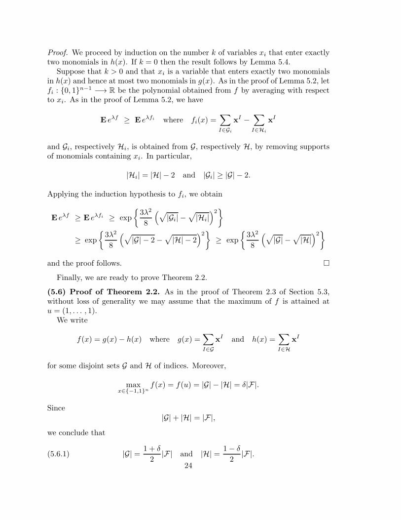
(5.6) Proof of Theorem 2.2. As in the proof of Theorem 2.3 of Section 5.3,without loss of generality we may assume that the maximum of f is attained atu = (1, . . . , 1).

We write

f(x) = g(x)− h(x) where g(x) =∑

I∈GxI and h(x) =

∑

I∈HxI

for some disjoint sets G and H of indices. Moreover,

maxx∈−1,1n

f(x) = f(u) = |G| − |H| = δ|F|.

Since|G|+ |H| = |F|,

we conclude that

(5.6.1) |G| = 1 + δ

2|F| and |H| = 1− δ

2|F|.

24

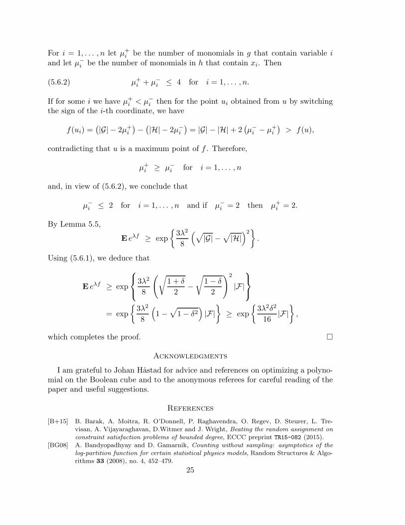
For i = 1, . . . , n let µ+i be the number of monomials in g that contain variable i

and let µ−i be the number of monomials in h that contain xi. Then

(5.6.2) µ+i + µ−

i ≤ 4 for i = 1, . . . , n.

If for some i we have µ+i < µ−

i then for the point ui obtained from u by switchingthe sign of the i-th coordinate, we have

f(ui) =(|G| − 2µ+

i

)−(|H| − 2µ−

i

)= |G| − |H|+ 2

(µ−i − µ+

i

)> f(u),

contradicting that u is a maximum point of f . Therefore,

µ+i ≥ µ−

i for i = 1, . . . , n

and, in view of (5.6.2), we conclude that

µ−i ≤ 2 for i = 1, . . . , n and if µ−

i = 2 then µ+i = 2.

By Lemma 5.5,

E eλf ≥ exp

3λ2

8

(√|G| −

√|H|)2

.

Using (5.6.1), we deduce that

E eλf ≥ exp

3λ2

8

(√1 + δ

2−√

1− δ

2

)2

|F|

= exp

3λ2

8

(1−

√1− δ2

)|F|

≥ exp

3λ2δ2

16|F|,

which completes the proof.

Acknowledgments

I am grateful to Johan Hastad for advice and references on optimizing a polyno-mial on the Boolean cube and to the anonymous referees for careful reading of thepaper and useful suggestions.

References

[B+15] B. Barak, A. Moitra, R. O’Donnell, P. Raghavendra, O. Regev, D. Steurer, L. Tre-visan, A. Vijayaraghavan, D.Witmer and J. Wright, Beating the random assignment on

constraint satisfaction problems of bounded degree, ECCC preprint TR15-082 (2015).

[BG08] A. Bandyopadhyay and D. Gamarnik, Counting without sampling: asymptotics of thelog-partition function for certain statistical physics models, Random Structures & Algo-

rithms 33 (2008), no. 4, 452–479.

25

[Ba15] A. Barvinok, Computing the partition function for cliques in a graph, Theory of Com-puting 11 (2015), Article 13, 339–355.

[Ba16] A. Barvinok, Computing the permanent of (some) complex matrices, Foundations of

Computational Mathematics 16 (2016), issue 2, 329–342.[BS14] A. Barvinok and P. Soberon, Computing the partition function for graph homomor-

phisms, preprint arXiv:1406.1771, to appear in Combinatorica (2014).[BS16] A. Barvinok and P. Soberon, Computing the partition function for graph homomorphisms

with multiplicities, Journal of Combinatorial Theory, Series A 137 (2016), 1–26.

[BH02] E. Boros and P.L. Hammer, Pseudo-Boolean optimization, Workshop on Discrete Opti-mization, DO’99 (Piscataway, NJ), Discrete Applied Mathematics 123 (2002), no. 1–3,

155–225.

[DS87] R.L. Dobrushin and S.B. Shlosman, Completely analytical interactions: constructivedescription, Journal of Statistical Physics 46 (1987), no. 5–6, 983–1014.

[Ha00] J. Hastad, On bounded occurrence constraint satisfaction, Information Processing Letters74 (2000), no. 1–2, 1–6.

[Ha01] J. Hastad, Some optimal inapproximability results, Journal of the ACM 48 (2001), no.

4, 798–859.[Ha15] J. Hastad, Improved bounds for bounded occurrence constraint satisfaction, manuscript,

available at https://www.nada.kth.se/∼johanh/bounded2.pdf (2005).

[HV04] J. Hastad and S. Venkatesh, On the advantage over a random assignment, RandomStructures & Algorithms 25 (2004), no. 2, 117–149.

[K+96] J. Kahn, N. Linial and A. Samorodnitsky, Inclusion-exclusion: exact and approximate,Combinatorica 16 (1996), no. 4, 465–477.

[KN12] S. Khot and A. Naor, Grothendieck-type inequalities in combinatorial optimization, Com-

munications on Pure and Applied Mathematics 65 (2012), no. 7, 992–1035.[LY52] T.D. Lee and C.N. Yang, Statistical theory of equations of state and phase transitions.

II. Lattice gas and Ising model, Physical Review (2) 87 (1952), 410–419.

[Re15] G. Regts, Zero-free regions of partition functions with applications to algorithms andgraph limits, preprint arXiv:1507.02089 (2015).

[We06] D. Weitz, Counting independent sets up to the tree threshold, STOC’06: Proceedings ofthe 38th Annual ACM Symposium on Theory of Computing, ACM, New York, 2006,

pp. 140–149.

[YL52] C.N. Yang and T.D. Lee, Statistical theory of equations of state and phase transitions.I. Theory of condensation, Physical Review (2) 87 (1952), 404–409.

[Zu07] D. Zuckerman, Linear degree extractors and the inapproximability of max clique and

chromatic number, Theory of Computing 3 (2007), 103–128.

Department of Mathematics, University of Michigan, Ann Arbor, MI 48109-1043,

USA

E-mail address: barvinok@umich.edu

26