Computer Arithmetic 1butler.cc.tut.fi/~piche/numa/lecture0304.pdf · Numerical Analysis, lecture 3:...

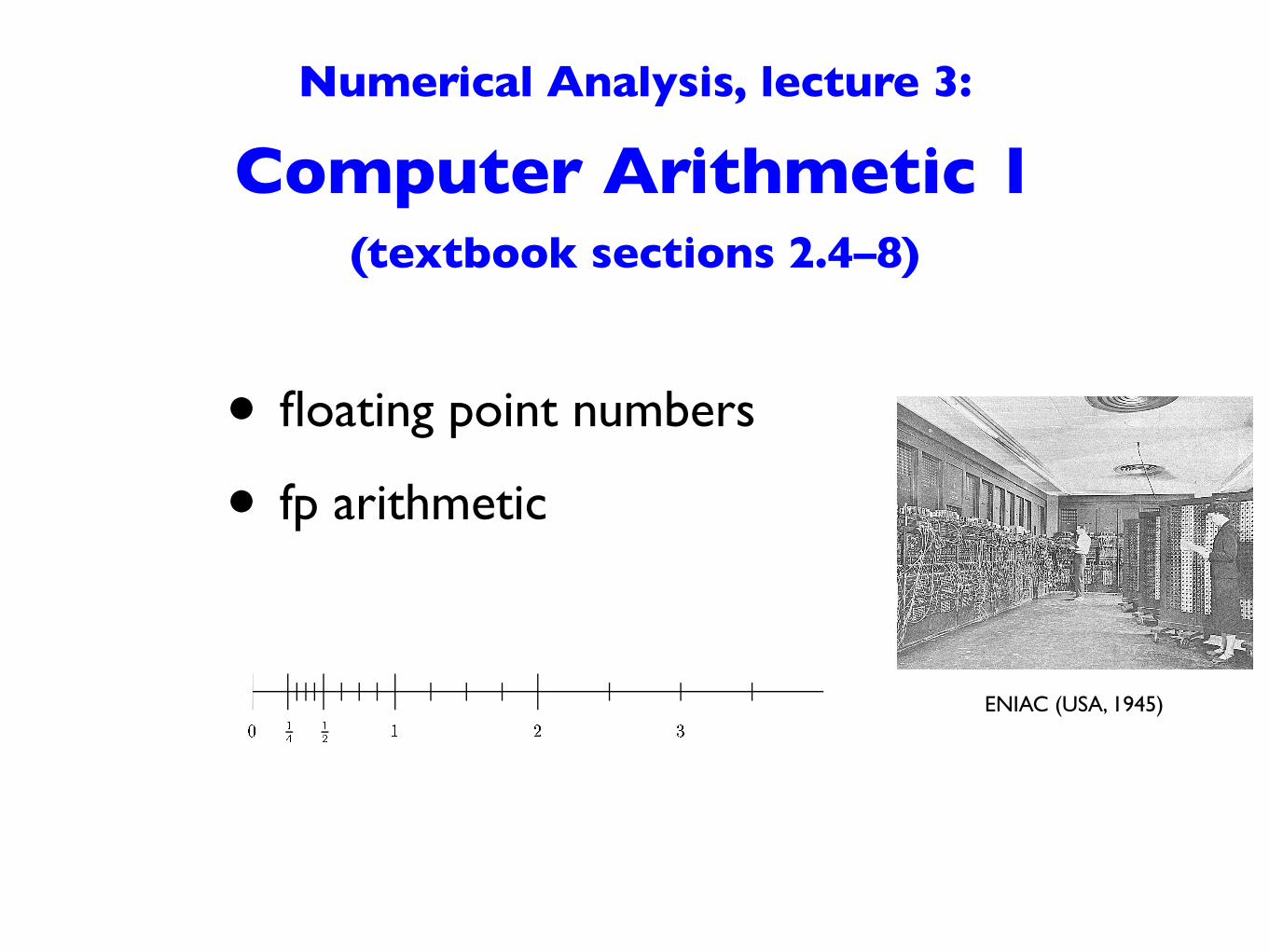
Numerical Analysis, lecture 3: Computer Arithmetic 1

(textbook sections 2.4–8)

• floating point numbers

• fp arithmetic

ENIAC (USA, 1945)

Numerical Analysis, lecture 3, slide ! 2

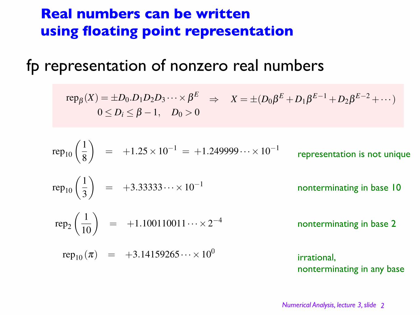
Real numbers can be written using floating point representation

fp representation of nonzero real numbers repβ (X) = ±D0.D1D2D3 · · ·×β E

0≤ Di ≤ β −1, D0 > 0

representation is not uniquerep10

�18

�= +1.25×10−1 = +1.249999 · · ·×10−1

nonterminating in base 10rep10

�13

�= +3.33333 · · ·×10−1

nonterminating in base 2rep2

�110

�= +1.100110011 · · ·×2−4

rep10 (π) = +3.14159265 · · ·×100irrational,nonterminating in any base

⇒ X = ±(D0β E +D1β E−1 +D2β E−2 + · · ·)


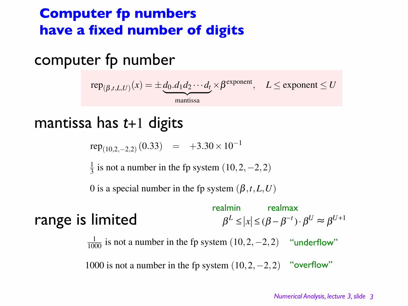
Computer fp numbers have a fixed number of digits

mantissa has t+1 digits

computer fp number

rep(10,2,−2,2) (0.33) = +3.30×10−1

13 is not a number in the fp system (10,2,−2,2)

0 is a special number in the fp system (β , t,L,U)

rep(β ,t,L,U)(x) = ±d0.d1d2 · · ·dt� �� mantissa

×β exponent, L≤ exponent≤U

11000 is not a number in the fp system (10,2,−2,2) “underflow”

1000 is not a number in the fp system (10,2,−2,2) “overflow”

! L " x " (! # !#t ) $ !U % !U+1range is limitedrealmin realmax


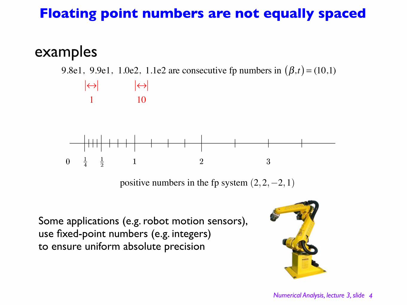
Floating point numbers are not equally spaced

9.8e1, 9.9e1, 1.0e2, 1.1e2 are consecutive fp numbers in !,t( ) = (10,1)

examples

!10

!1

positive numbers in the fp system (2,2,−2,1)

Some applications (e.g. robot motion sensors), use fixed-point numbers (e.g. integers) to ensure uniform absolute precision


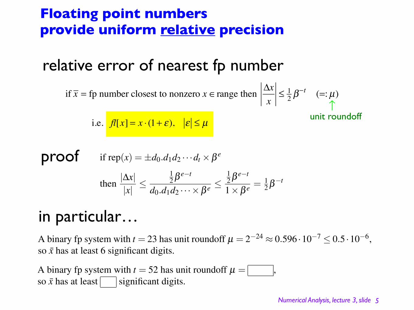
Floating point numbers provide uniform relative precision

if x = fp number closest to nonzero x !range then "xx

# 12 $

%t (=:µ)

relative error of nearest fp number

unit roundoff!

i.e. fl[x] = x ! (1+ "), " # µ

A binary fp system with t = 23 has unit roundoff µ = 2−24 ≈ 0.596 ·10−7 ≤ 0.5 ·10−6,so x has at least 6 significant digits.

in particular…

A binary fp system with t = 52 has unit roundoff µ = ,so x has at least significant digits.

proof if rep(x) = ±d0.d1d2 · · ·dt ×β e

then|∆x||x| ≤

12 β e−t

d0.d1d2 · · ·×β e ≤12 β e−t

1×β e = 12 β−t


IEEE standard 754 is implemented in modern scientific computers

+!, "! (overflow or divide by zero)

NaN (not a number, e.g. 0/0, 0!∞)

special numbers+0, ! 0 (zero or underflow)

subnormal (to allow “gradual underflow”)

normal numbers

!, t, L,U( ) = (2, 23, "126, 127)µ = 2"24 # 6 $10"8

[2"126, 2128 )# [1.2 $10"38, 3.4 $1038 )

single precision (32 bit)

!, t, L,U( ) = (2, 52, "1022, 1023)µ = 2"53 #1 $10"16

[2"1022, 21024 )# [2.2 $10"308, 1.8 $10308 )

double precision (64 bit)


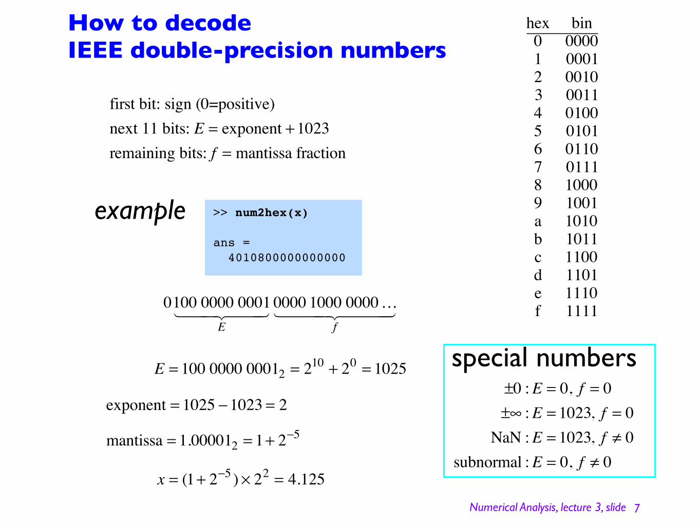
How to decode IEEE double-precision numbers

hex bin0 00001 00012 00103 00114 01005 01016 01107 01118 10009 1001a 1010b 1011c 1100d 1101e 1110f 1111

first bit: sign (0=positive)next 11 bits: E = exponent +1023remaining bits: f = mantissa fraction

example >> num2hex(x)

ans = 4010800000000000

0100 0000 0001E

! "## $## 0000 1000 0000…f

! "### $###

E = 100 0000 00012 = 210 + 20 = 1025

exponent = 1025 !1023 = 2

mantissa = 1.000012 = 1+ 2!5

x = (1+ 2!5 ) " 22 = 4.125

special numbers±0 :E = 0, f = 0±! :E = 1023, f = 0NaN :E = 1023, f " 0

subnormal :E = 0, f " 0


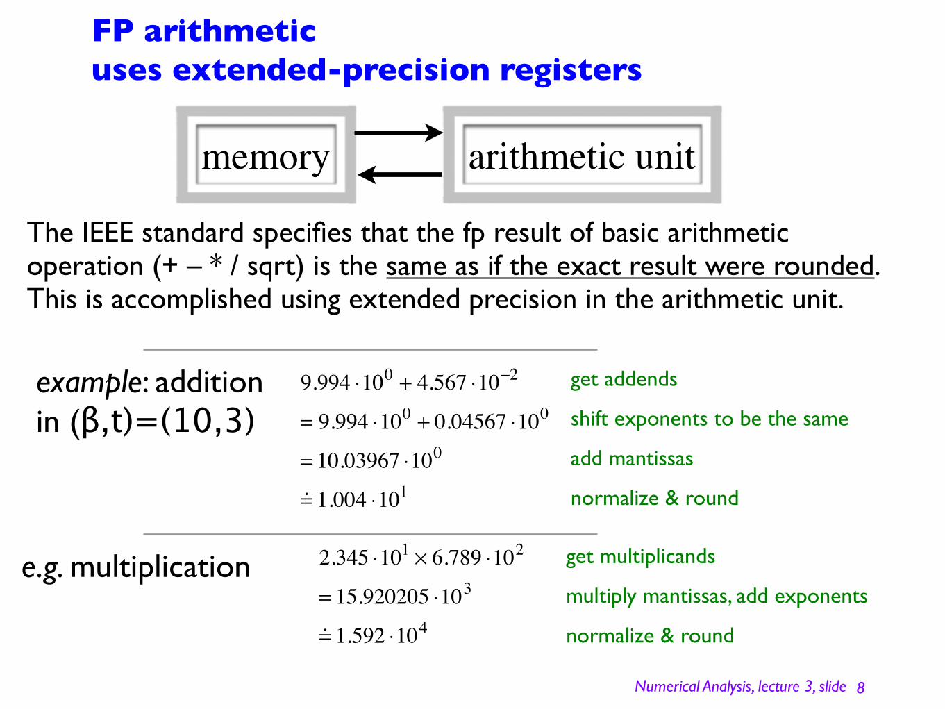
FP arithmetic uses extended-precision registers

get addends

shift exponents to be the same

add mantissas

normalize & round

get multiplicands

multiply mantissas, add exponents

normalize & round

memory arithmetic unit

The IEEE standard specifies that the fp result of basic arithmetic operation (+ – * / sqrt) is the same as if the exact result were rounded. This is accomplished using extended precision in the arithmetic unit.

example: additionin (β,t)=(10,3)

9.994 !100 + 4.567 !10"2

= 9.994 !100 + 0.04567 !100

= 10.03967 !100

! 1.004 !101

e.g. multiplication

2.345 !101 " 6.789 !102

= 15.920205 !103

! 1.592 !104

Numerical Analysis, lecture 3, slide !

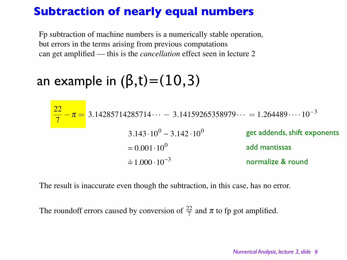
Subtraction of nearly equal numbers

9

get addends, shift exponents

add mantissas

normalize & round

Fp subtraction of machine numbers is a numerically stable operation,but errors in the terms arising from previous computationscan get amplified — this is the cancellation effect seen in lecture 2

3.143 !100 " 3.142 !100

= 0.001 !100

! 1.000 !10"3

an example in (β,t)=(10,3)227−π = 3.14285714285714 · · · − 3.14159265358979 · · · = 1.264489 · · · · 10−3

The result is inaccurate even though the subtraction, in this case, has no error.

The roundoff errors caused by conversion of 227 and π to fp got amplified.


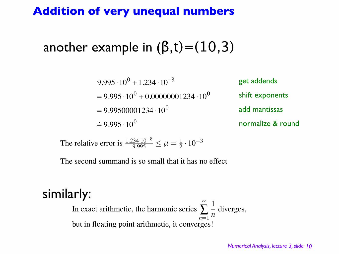
Addition of very unequal numbers

10

another example in (β,t)=(10,3)

9.995 !100 +1.234 !10"8

= 9.995 !100 + 0.00000001234 !100

= 9.99500001234 !100

! 9.995 !100

get addends

shift exponents

add mantissas

normalize & round

similarly:In exact arithmetic, the harmonic series

∞

∑n=1

1n

diverges,

but in floating point arithmetic, it converges!

The second summand is so small that it has no effect

The relative error is 1.234·10−8

9.995 ≤ µ = 12 · 10−3


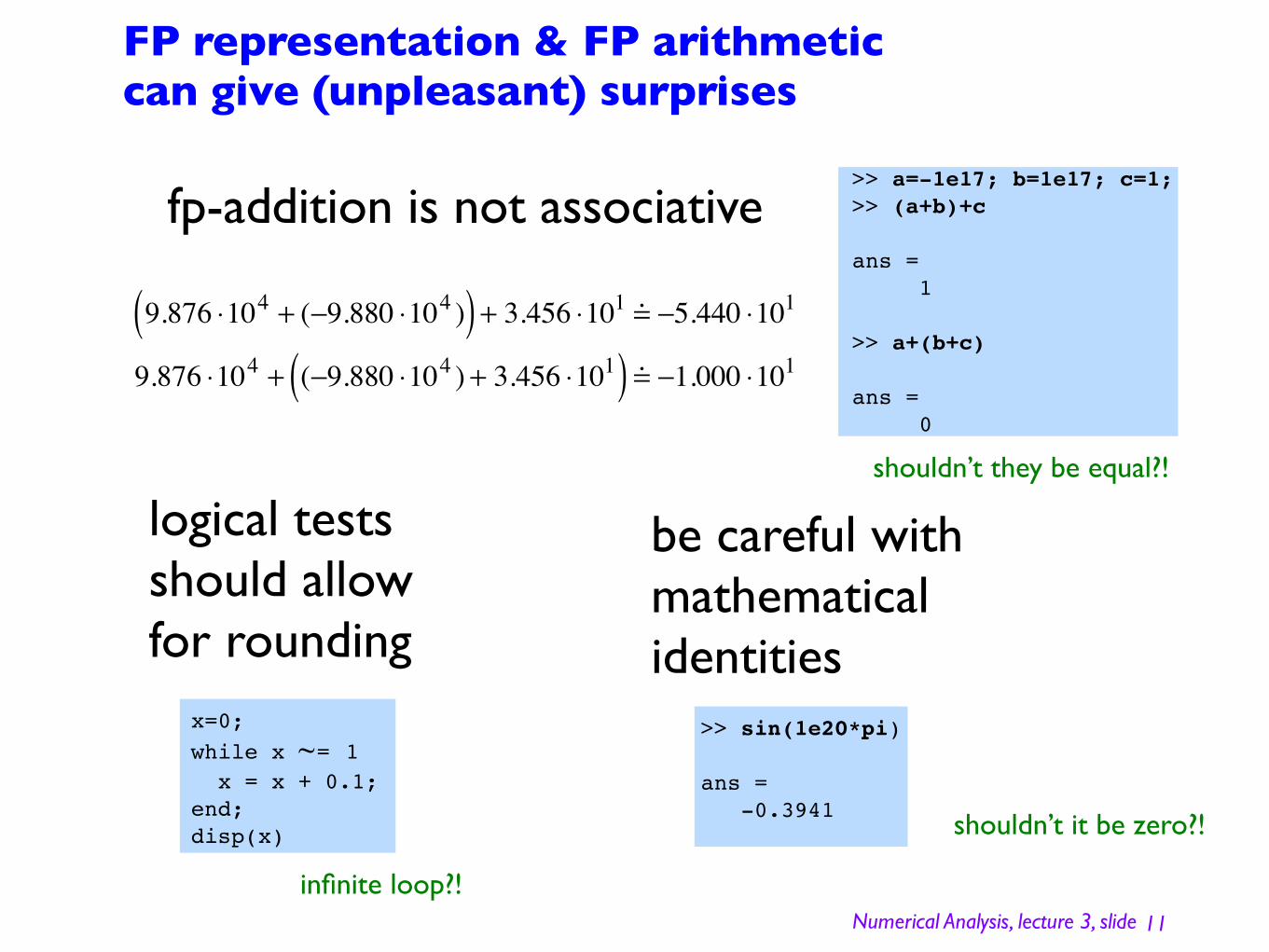
FP representation & FP arithmeticcan give (unpleasant) surprises

fp-addition is not associative

9.876 !104 + ("9.880 !104 )( ) + 3.456 !101 ! "5.440 !1019.876 !104 + ("9.880 !104 ) + 3.456 !101( ) ! "1.000 !101

logical tests should allow for rounding

x=0;

while x ~= 1 x = x + 0.1; end; disp(x)

infinite loop?!

be careful with mathematicalidentities

>> sin(1e20*pi)

ans = -0.3941

shouldn’t it be zero?!

>> a=-1e17; b=1e17; c=1;>> (a+b)+c

ans = 1

>> a+(b+c)

ans = 0

shouldn’t they be equal?!


what happened, what’s next

• floating point representation relative error ≤ μ=½β-t

• IEEE standard for fp arithmetic

• be aware of

- binary arithmetic

- finite precision (mantissa)

- finite exponents

Next: error propagation (§2.7)

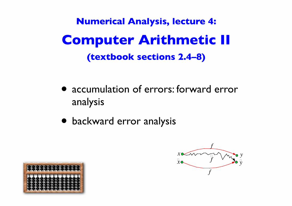
Numerical Analysis, lecture 4: Computer Arithmetic II

(textbook sections 2.4–8)

• accumulation of errors: forward error analysis

• backward error analysis

f

f

f^^

x^^x

y^^y


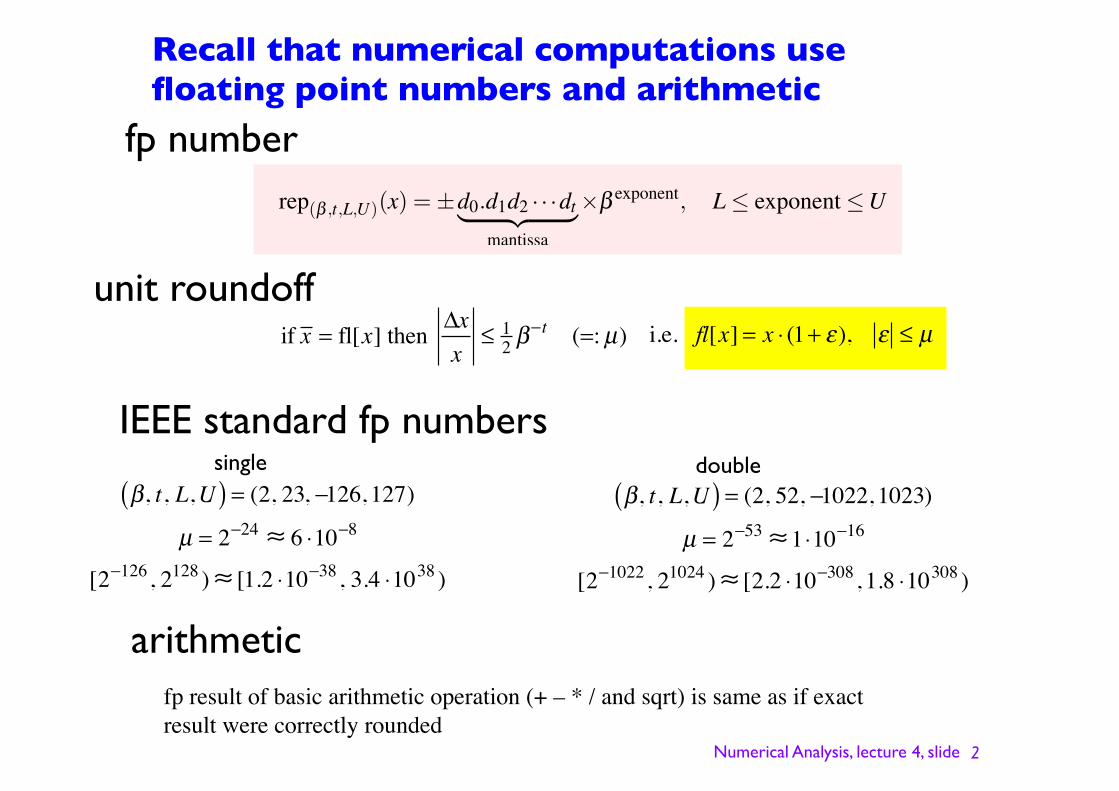
Recall that numerical computations use floating point numbers and arithmetic

2

fp numberrep(β ,t,L,U)(x) = ±d0.d1d2 · · ·dt� ��

mantissa

×β exponent, L≤ exponent≤U

IEEE standard fp numbers

!, t, L,U( ) = (2, 23, "126, 127)µ = 2"24 # 6 $10"8

[2"126, 2128 )# [1.2 $10"38, 3.4 $1038 )

single!, t, L,U( ) = (2, 52, "1022, 1023)

µ = 2"53 #1 $10"16[2"1022, 21024 )# [2.2 $10"308, 1.8 $10308 )

double

fp result of basic arithmetic operation (+ – * / and sqrt) is same as if exact result were correctly rounded

arithmetic

if x = fl[x] then !xx

" 12 #

$t (=:µ) i.e. fl[x] = x ! (1+ "), " # µ

unit roundoff


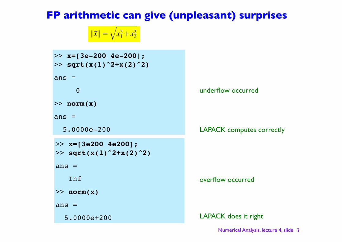
FP arithmetic can give (unpleasant) surprises

3

>> x=[3e-200 4e-200]; >> sqrt(x(1)^2+x(2)^2)

ans =

0

>> norm(x)

ans =

5.0000e-200

underflow occurred

LAPACK computes correctly

��x� =�

x21 + x2

2

overflow occurred

LAPACK does it right

>> x=[3e200 4e200];>> sqrt(x(1)^2+x(2)^2)

ans =

Inf

>> norm(x)

ans =

5.0000e+200


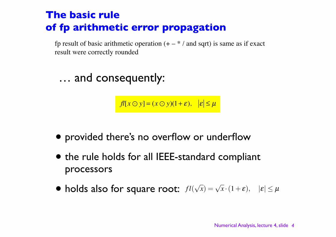
The basic rule of fp arithmetic error propagation

fl[x! y] = (x! y)(1+ !), ! " µ

fp result of basic arithmetic operation (+ – * / and sqrt) is same as if exact result were correctly rounded

… and consequently:

• provided there’s no overflow or underflow

• the rule holds for all IEEE-standard compliant processors

• holds also for square root: f l(√

x) =√

x · (1+ ε), |ε|≤ µ


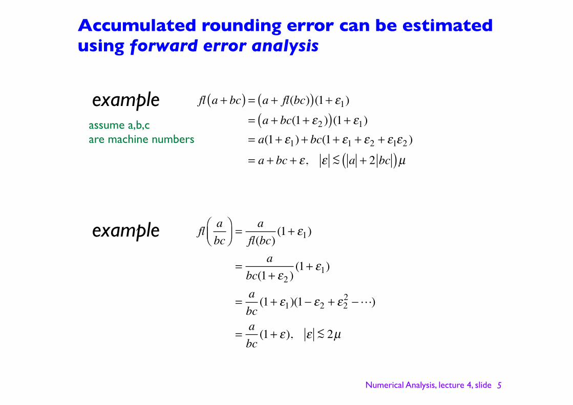
Accumulated rounding error can be estimated using forward error analysis

exampleassume a,b,care machine numbers

fl a + bc( ) = a + fl(bc)( )(1+ !1)= a + bc(1+ !2 )( )(1+ !1)= a(1+ !1) + bc(1+ !1 + !2 + !1!2 )

= a + bc + !, ! <~ a + 2 bc( )µ

fl abc

!"#

$%&=

afl(bc)

(1+ '1)

=a

bc(1+ '2 )(1+ '1)

=abc(1+ '1)(1( '2 + '2

2 (!)

=abc(1+ '), ' <~ 2µ

example


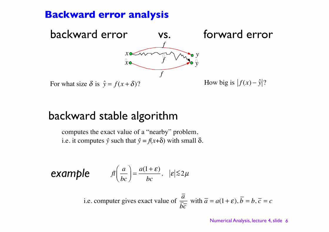
Backward error analysis

backward error vs. forward error

How big is f (x) ! y ?For what size ! is y = f (x + ! )?

f

f

f^^

x^^x

y^^y

backward stable algorithmcomputes the exact value of a “nearby” problem,i.e. it computes ! such that ! = f(x+!) with small !.

fl abc

!"#

$%&=a(1+ ')bc

, ' <~2µexample

i.e. computer gives exact value of abc

with a = a(1+ !), b = b, c = c


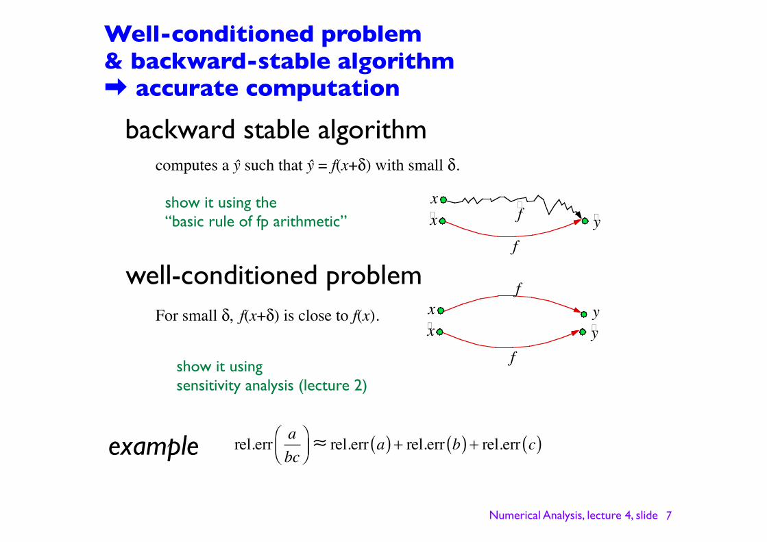
Well-conditioned problem & backward-stable algorithm ➡ accurate computation

backward stable algorithmcomputes a ! such that ! = f(x+!) with small !.

f

f^^

x^^x

y^^

well-conditioned problemFor small !, f(x+!) is close to f(x).

f

fx^^x

y^^y

rel.err abc

!"#

$%&' rel.err a( ) + rel.err b( ) + rel.err c( )example

show it using the“basic rule of fp arithmetic”

show it using sensitivity analysis (lecture 2)


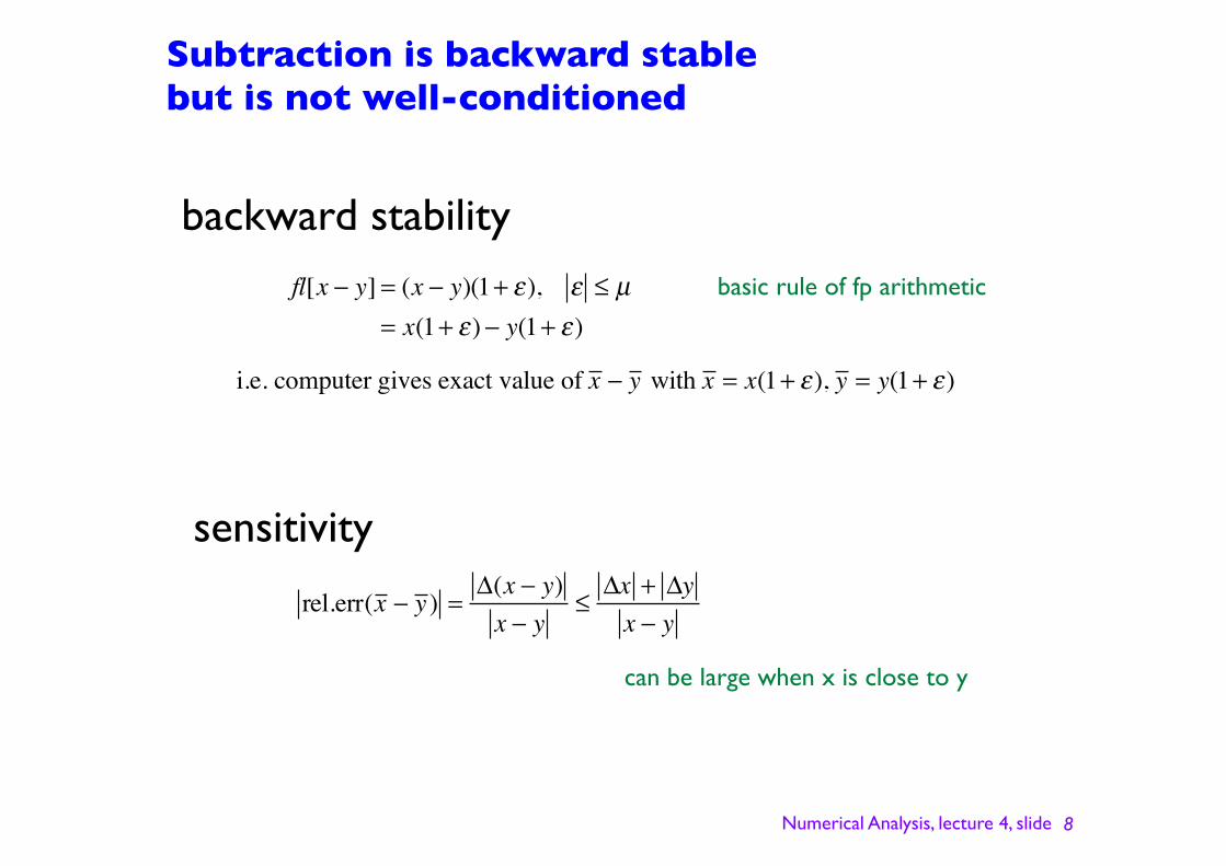
Subtraction is backward stablebut is not well-conditioned

backward stability

can be large when x is close to y

fl[x ! y] = (x ! y)(1+ "), " # µ= x(1+ ") ! y(1+ ")

i.e. computer gives exact value of x ! y with x = x(1+ "), y = y(1+ ")

sensitivity

rel.err(x ! y ) ="(x ! y)x ! y

#"x + "yx ! y

basic rule of fp arithmetic


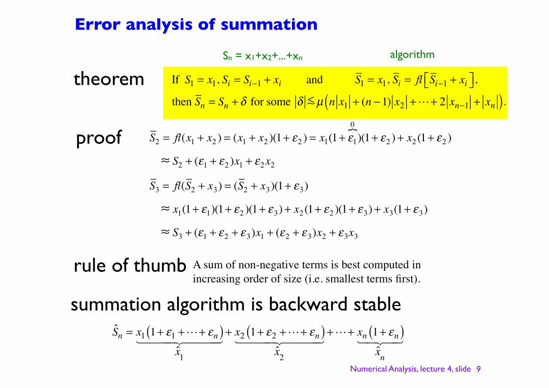
Error analysis of summation

rule of thumb A sum of non-negative terms is best computed in increasing order of size (i.e. smallest terms first).

theoremalgorithm

If S1 = x1, Si = Si!1 + xi and S1 = x1, Si = fl Si!1 + xi"# $%,

then Sn = Sn + & for some & <!µ n x1 + (n !1) x2 +"+ 2 xn!1 + xn( ).

proof

S2 = fl(x1 + x2 ) = (x1 + x2 )(1+ !2 ) = x1(1+ !10!)(1+ !2 ) + x2 (1+ !2 )

" S2 + (!1 + !2 )x1 + !2x2

S3 = fl(S2 + x3) = (S2 + x3)(1+ !3)

" x1(1+ !1)(1+ !2 )(1+ !3) + x2 (1+ !2 )(1+ !3) + x3(1+ !3)

" S3 + (!1 + !2 + !3)x1 + (!2 + !3)x2 + !3x3

summation algorithm is backward stable

Sn = x1 1+ !1 +!+ !n( )x1

" #$$$ %$$$+ x2 1+ !2 +!+ !n( )

x2" #$$$ %$$$

+!+ xn 1+ !n( )xn

" #$ %$

Sn = x1+x2+...+xn


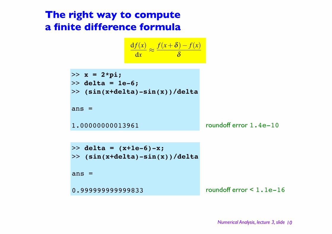
The right way to compute a finite difference formula

10

d f (x)dx

≈ f (x+δ )− f (x)δ

>> x = 2*pi;>> delta = 1e-6;>> (sin(x+delta)-sin(x))/delta

ans =

1.00000000013961 roundoff error 1.4e-10

>> delta = (x+1e-6)-x;>> (sin(x+delta)-sin(x))/delta

ans =

0.999999999999833 roundoff error < 1.1e-16


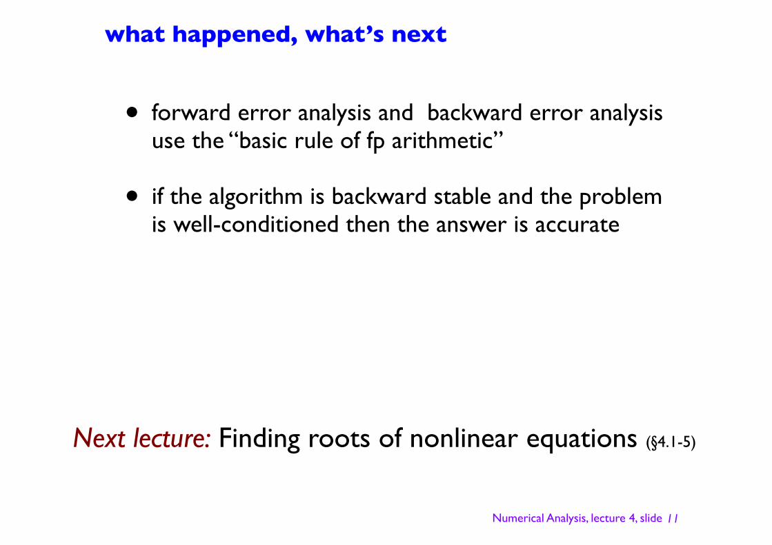
what happened, what’s next

• forward error analysis and backward error analysis use the “basic rule of fp arithmetic”

• if the algorithm is backward stable and the problem is well-conditioned then the answer is accurate

Next lecture: Finding roots of nonlinear equations (§4.1-5)

Computer Arithmetic 1butler.cc.tut.fi/~piche/numa/lecture0304.pdf · Numerical Analysis, lecture 3:...

Documents

Transcript of Computer Arithmetic 1butler.cc.tut.fi/~piche/numa/lecture0304.pdf · Numerical Analysis, lecture 3:...