Computational Physics Praktikum: Numerische Hydrodynamikkley/... · Computational Physics...

Computational Physics Praktikum:Numerische Hydrodynamik

Wilhelm KleyInstitut fur Astronomie & Astrophysik

& Kepler Center for Astro and Particle Physics Tubingen

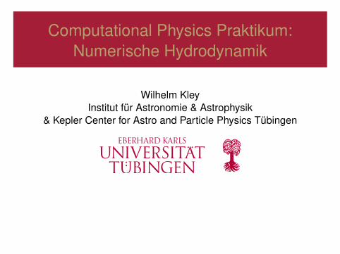
Hydrodynamik: Hydrodynamische GleichungenDie Euler-Gleichungen der Hydrodynamik lauten in Erhaltungsform

∂ρ

∂t+∇·(ρ~u) = 0 (1)

∂(ρ~u)

∂t+∇·(ρ~u ⊗ ~u) = −∇p + ρ~k (2)

∂(ρε)

∂t+∇·(ρε~u) = −p∇·~u (3)

~u: Geschwindigkeit, ~k : außere Krafte, ε innere spezifische EnergieDie Gleichungen beschreiben die Erhaltung der Masse, Impuls und Energie.Vervollstandigung durch Zustandsgleichung:

p = (γ − 1) ρε (4)

Forme damit die Energie-Gleichung (3) in eine Gl. fur den Druck um

∂p∂t

+∇·(p~u) = −(γ − 1)p∇ · ~u (5)

W. Kley Computational Physics Praktikum 2

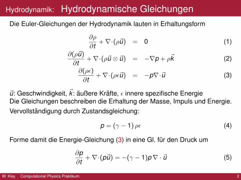
Hydrodynamik: UmschreibenEntwickle die Divergenzen auf der linken Seite und benutze fur die Impuls-und Energiegleichung die Kontinuitatgleichung

∂ρ

∂t+ (~u · ∇)ρ = −ρ∇ · ~u (6)

∂~u∂t

+ (~u · ∇)~u = −1ρ∇p + ~k (7)

∂p∂t

+ (~u · ∇)p = −γp∇·~u (8)

Da alle Großen Funktionen von Ort (~r ) und Zeit (t) sind, z.B. ρ(~r , t), kann furdie linke Seite die totale Zeitableitung geschrieben werden.z.B. fur die Dichte

DρDt

=∂ρ

∂t+ (~u · ∇)ρ = −ρ∇ ·~u (9)

der OperatorDDt

=∂

∂t+ ~u · ∇ (10)

heißt substantielle Zeitableitung (entspricht der totalen Zeitableitung, d/dt)W. Kley Computational Physics Praktikum 3

Hydrodynamik: Lagrange-Formulierung

Benutze die substantielle Ableitung

DρDt

= −ρ∇ · ~u (11)

D~uDt

= −1ρ∇p + ~k (12)

DpDt

= −γp∇·~u (13)

Beschreibt zeitliche Anderung der Großen in einem mit der Stromungmitbewegten System = Lagrange-FormulierungDie Lagrangeformulierung kann z.B. gut bei radialenStern-Oszillationen verwendet werden.Ist 1D Problem. Hier durch mitbewegte Masseschalen

Bei Euler-Formulierung (auf Gitter): orstfest !


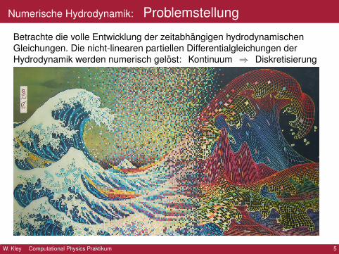
Numerische Hydrodynamik: Problemstellung

Betrachte die volle Entwicklung der zeitabhangigen hydrodynamischenGleichungen. Die nicht-linearen partiellen Differentialgleichungen derHydrodynamik werden numerisch gelost: Kontinuum ⇒ Diskretisierung


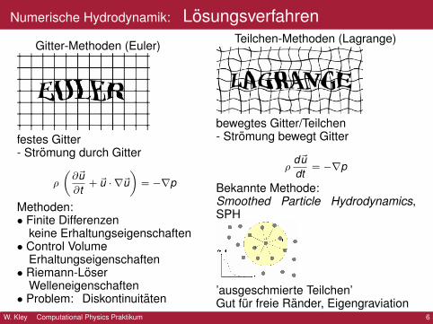
Numerische Hydrodynamik: Losungsverfahren

Gitter-Methoden (Euler)

festes Gitter- Stromung durch Gitter

ρ

(∂~u∂t

+ ~u · ∇~u)

= −∇p

Methoden:• Finite Differenzen

keine Erhaltungseigenschaften• Control Volume

Erhaltungseigenschaften• Riemann-Loser

Welleneigenschaften• Problem: Diskontinuitaten

Teilchen-Methoden (Lagrange)

bewegtes Gitter/Teilchen- Stromung bewegt Gitter

ρd~udt

= −∇p

Bekannte Methode:Smoothed Particle Hydrodynamics,SPH

’ausgeschmierte Teilchen’Gut fur freie Rander, Eigengraviation


Numerische Hydrodynamik: betrachte: 1D Eulergleichungen

Beschreiben Erhaltung von: Masse, Impuls und Energie

∂ρ

∂t+∂ρu∂x

= 0 (14)

∂ρu∂t

+∂ρuu∂x

= −∂p∂x

(15)

∂ρε

∂t+∂ρεu∂x

= −p∂u∂x

(16)

ρ: Dichteu: Geschwindigkeitp: Druckε: innere spezifische Energie (Energie/Masse)Mit Zustandsgleichung

p = (γ − 1)ρε (17)

γ: AdiabatenexponentPartielle Dgl. in Raum und Zeit.→ Brauche Diskretisierung in Raum und Zeit.


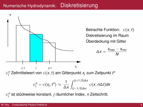
Numerische Hydrodynamik: Diskretisierung

Xj−1 j j+1

ψ

Betrachte Funktion: ψ(x , t)Diskretisierung im RaumUberdeckung mit Gitter

∆x =xmax − xmin

N

ψnj Zellmittelwert von ψ(x , t) am Gitterpunkt xj zum Zeitpunkt tn

ψnj = ψ(xj , tn) ≈ 1

∆x

∫ (j+1/2)∆x

(j−1/2)∆xψ(x ,n∆t)dx

ψnj ist stuckweise konstant. j raumlicher Index, n Zeitschritt.


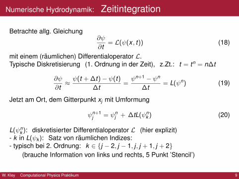
Numerische Hydrodynamik: Zeitintegration

Betrachte allg. Gleichung∂ψ

∂t= L(ψ(x , t)) (18)

mit einem (raumlichen) Differentialoperator L.Typische Diskretisierung (1. Ordnung in der Zeit), z.Zt.: t = tn = n∆t

∂ψ

∂t≈ ψ(t + ∆t)− ψ(t)

∆t=ψn+1 − ψn

∆t= L(ψn) (19)

Jetzt am Ort, dem Gitterpunkt xj mit Umformung

ψn+1j = ψn

j + ∆tL(ψnk ) (20)

L(ψnk ): diskretisierter Differentialoperator L (hier explizit)

- k in L(ψk ): Satz von raumlichen Indizes:- typisch bei 2. Ordnung: k ∈ {j − 2, j − 1, j , j + 1, j + 2}

(brauche Information von links und rechts, 5 Punkt ’Stencil’)


Numerische Hydrodynamik: Operator-Splitting

∂~A∂t

= L1(~A) + L2(~A) (21)

Li (~A), i = 1,2 einzelne (Differential-)Operatorenangewandt auf die Großen ~A = (ρ,u, ε).Hier bei 1D idealer Hydrodynamik

L1 : Advektion

L2 : Druck, bzw. ext. Krafte

Zur Losung in einzelne Unterschritte unterteilt

~A1 = ~An + ∆tL1(~An)

~An+1 = ~A2 = ~A1 + ∆tL2(~A1) (22)

Li ist Differenzenoperator zu Li .


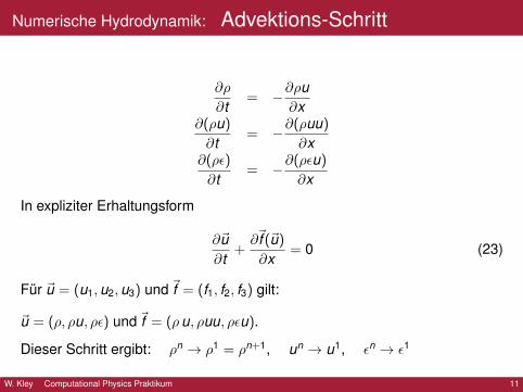
Numerische Hydrodynamik: Advektions-Schritt

∂ρ

∂t= −∂ρu

∂x∂(ρu)

∂t= −∂(ρuu)

∂x∂(ρε)

∂t= −∂(ρεu)

∂x

In expliziter Erhaltungsform

∂~u∂t

+∂~f (~u)

∂x= 0 (23)

Fur ~u = (u1,u2,u3) und ~f = (f1, f2, f3) gilt:

~u = (ρ, ρu, ρε) und ~f = (ρu, ρuu, ρεu).

Dieser Schritt ergibt: ρn → ρ1 = ρn+1, un → u1, εn → ε1


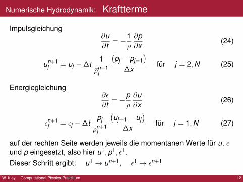
Numerische Hydrodynamik: Kraftterme

Impulsgleichung∂u∂t

= −1ρ

∂p∂x

(24)

un+1j = uj −∆t

1ρn+1

j

(pj − pj−1

)∆x

fur j = 2,N (25)

Energiegleichung∂ε

∂t= −p

ρ

∂u∂x

(26)

εn+1j = εj −∆t

pj

ρn+1j

(uj+1 − uj

)∆x

fur j = 1,N (27)

auf der rechten Seite werden jeweils die momentanen Werte fur u, εund p eingesetzt, also hier u1,p1, ε1.Dieser Schritt ergibt: u1 → un+1, ε1 → εn+1


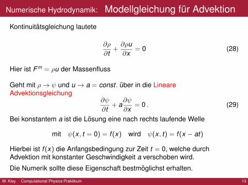
Numerische Hydrodynamik: Modellgleichung fur Advektion

Kontinuitatsgleichung lautete

∂ρ

∂t+∂ρu∂x

= 0 (28)

Hier ist F m = ρu der Massenfluss

Geht mit ρ→ ψ und u → a = const . uber in die LineareAdvektionsgleichung

∂ψ

∂t+ a

∂ψ

∂x= 0 . (29)

Bei konstantem a ist die Losung eine nach rechts laufende Welle

mit ψ(x , t = 0) = f (x) wird ψ(x , t) = f (x − at)

Hierbei ist f (x) die Anfangsbedingung zur Zeit t = 0, welche durchAdvektion mit konstanter Geschwindigkeit a verschoben wird.

Die Numerik sollte diese Eigenschaft bestmoglichst erhalten.


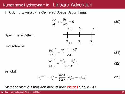
Numerische Hydrodynamik: Lineare AdvektionFTCS: Forward Time Centered Space Algorithmus

∂ψ

∂t+ a

∂ψ

∂x= 0 (30)

Spezifiziere Gitter :

x xxj+1jj−1

ψψj j+1

ψj−1

und schreibe∂ψ

∂t

∣∣∣∣nj

=ψn+1

j − ψnj

∆t(31)

∂ψ

∂x

∣∣∣∣nj

=ψn

j+1 − ψnj−1

2 ∆x(32)

es folgt

ψn+1j = ψn

j −a∆t2∆x

(ψn

j+1 − ψnj−1)

(33)

Methode sieht gut motiviert aus: ist aber Instabil fur alle ∆t !W. Kley Computational Physics Praktikum 14

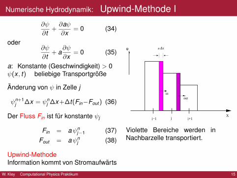
Numerische Hydrodynamik: Upwind-Methode I∂ψ

∂t+∂aψ∂x

= 0 (34)

oder∂ψ

∂t+ a

∂ψ

∂x= 0 (35)

a: Konstante (Geschwindigkeit) > 0ψ(x , t) beliebige Transportgroße

Anderung von ψ in Zelle j

ψn+1j ∆x = ψn

j ∆x+∆t(Fin−Fout ) (36)

Der Fluss Fin ist fur konstante ψj

Fin = aψnj−1 (37)

Fout = aψnj (38)

Upwind-MethodeInformation kommt von Stromaufwarts

outin

∆ψ tα

X

a

j−1 j j+1

Violette Bereiche werden inNachbarzelle transportiert.


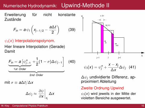
Numerische Hydrodynamik: Upwind-Methode IIErweiterung fur nicht konstanteZustande

Fin = aψI

(xj−1/2 −

a∆t2

)(39)

ψI(x) Interpolationspolynom.Hier lineare Interpolation (Gerade)Damit

Fin = a[ψn

j−1︸︷︷︸1st Order

+12

(1− σ)∆ψj−1

]︸︷︷︸

2nd Order

(40)

mit σ ≡ a∆t/∆x

∆ψj ≈∂ψ

∂x

∣∣∣∣xj

∆x

out

in

∆ψ tα

X

a

j−1 j j+1

ψ (x)I

ψI(x) = ψnj +

x − xj

∆x∆ψj (41)

∆ψj undividierte Differenz, ap-proximiert Ableitung

Zweite Ordnung UpwindψI(x) wird jeweils in der Mitte dervioletten Bereiche ausgewertet.


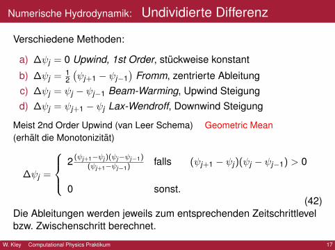
Numerische Hydrodynamik: Undividierte Differenz

Verschiedene Methoden:

a) ∆ψj = 0 Upwind, 1st Order, stuckweise konstant

b) ∆ψj = 12

(ψj+1 − ψj−1

)Fromm, zentrierte Ableitung

c) ∆ψj = ψj − ψj−1 Beam-Warming, Upwind Steigungd) ∆ψj = ψj+1 − ψj Lax-Wendroff, Downwind Steigung

Meist 2nd Order Upwind (van Leer Schema) Geometric Mean(erhalt die Monotonizitat)

∆ψj =

2 (ψj+1−ψj )(ψj−ψj−1)

(ψj+1−ψj−1) falls (ψj+1 − ψj)(ψj − ψj−1) > 0

0 sonst.(42)

Die Ableitungen werden jeweils zum entsprechenden Zeitschrittlevelbzw. Zwischenschritt berechnet.


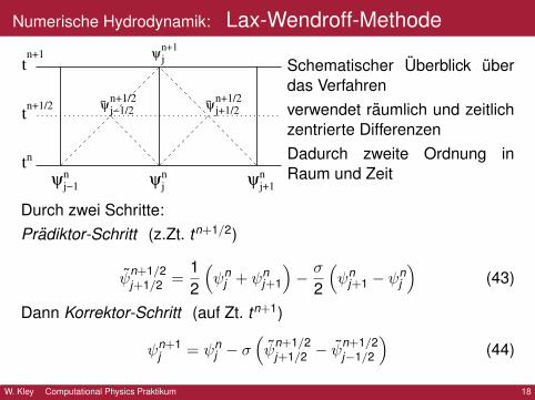
Numerische Hydrodynamik: Lax-Wendroff-Methode

n

n+1

nn

t

t

tn

n+1

n+1/2 ~ ~

ψ

ψ ψ

ψψ ψ

n+1/2n+1/2

j

j+1jj−1

j−1/2 j+1/2

Schematischer Uberblick uberdas Verfahrenverwendet raumlich und zeitlichzentrierte DifferenzenDadurch zweite Ordnung inRaum und Zeit

Durch zwei Schritte:Pradiktor-Schritt (z.Zt. tn+1/2)

ψn+1/2j+1/2 =

12

(ψn

j + ψnj+1

)− σ

2

(ψn

j+1 − ψnj

)(43)

Dann Korrektor-Schritt (auf Zt. tn+1)

ψn+1j = ψn

j − σ(ψ

n+1/2j+1/2 − ψ

n+1/2j−1/2

)(44)


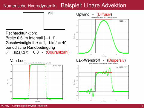
Numerische Hydrodynamik: Beispiel: Linare Advektion(x)ψ

Rechteckfunktion:Breite 0.6 im Intervall [−1,1]Geschwindigkeit a = 1, bis t = 40periodische Randbedingungσ = a∆t/∆x = 0.8 - (Courantzahl)

Upwind - (Diffusiv)

0

0.2

0.4

0.6

0.8

1

-1 -0.5 0 0.5 1

Ph

i-A

ch

se

X-Achse

Linear Advection (N=600,t=40): Upwind, sigma=0.8

AnalyticUpwind

Van Leer

0

0.2

0.4

0.6

0.8

1

-1 -0.5 0 0.5 1

Ph

i-A

ch

se

X-Achse

Linear Advection (N=600,t=40): Van Leer, sigma=0.8

AnalyticVan Leer

Lax-Wendroff - (Dispersiv)

-0.4

-0.2

0

0.2

0.4

0.6

0.8

1

1.2

1.4

-1 -0.5 0 0.5 1

Ph

i-A

ch

se

X-Achse

Linear Advection (N=600,t=40): Lax Wendroff, sigma=0.8

AnalyticLax Wendroff


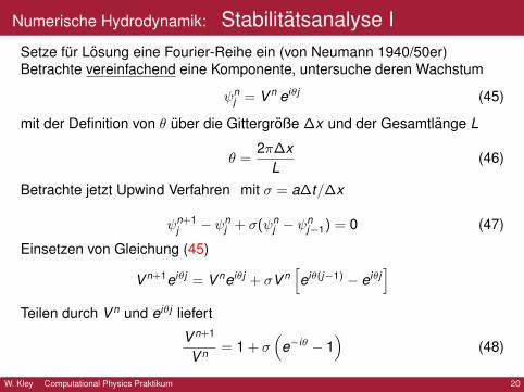
Numerische Hydrodynamik: Stabilitatsanalyse ISetze fur Losung eine Fourier-Reihe ein (von Neumann 1940/50er)Betrachte vereinfachend eine Komponente, untersuche deren Wachstum

ψnj = V n eiθj (45)

mit der Definition von θ uber die Gittergroße ∆x und der Gesamtlange L

θ =2π∆x

L(46)

Betrachte jetzt Upwind Verfahren mit σ = a∆t/∆x

ψn+1j − ψn

j + σ(ψnj − ψn

j−1) = 0 (47)

Einsetzen von Gleichung (45)

V n+1eiθj = V neiθj + σV n[eiθ(j−1) − eiθj

]Teilen durch V n und eiθj liefert

V n+1

V n = 1 + σ(

e−iθ − 1)

(48)


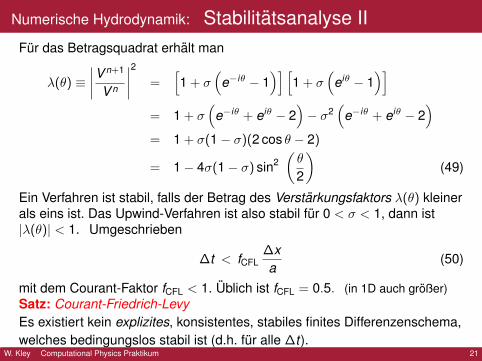
Numerische Hydrodynamik: Stabilitatsanalyse IIFur das Betragsquadrat erhalt man

λ(θ) ≡∣∣∣∣V n+1

V n

∣∣∣∣2 =[1 + σ

(e−iθ − 1

)] [1 + σ

(eiθ − 1

)]= 1 + σ

(e−iθ + eiθ − 2

)− σ2

(e−iθ + eiθ − 2

)= 1 + σ(1− σ)(2 cos θ − 2)

= 1− 4σ(1− σ) sin2(θ

2

)(49)

Ein Verfahren ist stabil, falls der Betrag des Verstarkungsfaktors λ(θ) kleinerals eins ist. Das Upwind-Verfahren ist also stabil fur 0 < σ < 1, dann ist|λ(θ)| < 1. Umgeschrieben

∆t < fCFL∆xa

(50)

mit dem Courant-Faktor fCFL < 1. Ublich ist fCFL = 0.5. (in 1D auch großer)Satz: Courant-Friedrich-LevyEs existiert kein explizites, konsistentes, stabiles finites Differenzenschema,welches bedingungslos stabil ist (d.h. fur alle ∆t).


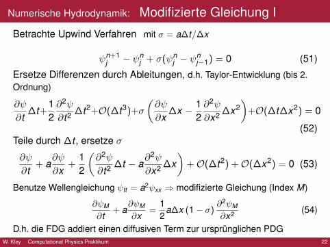
Numerische Hydrodynamik: Modifizierte Gleichung I

Betrachte Upwind Verfahren mit σ = a∆t/∆x

ψn+1j − ψn

j + σ(ψnj − ψ

nj−1) = 0 (51)

Ersetze Differenzen durch Ableitungen, d.h. Taylor-Entwicklung (bis 2.Ordnung)

∂ψ

∂t∆t+

12∂2ψ

∂t2 ∆t2+O(∆t3)+σ

(∂ψ

∂x∆x − 1

2∂2ψ

∂x2 ∆x2)

+O(∆t∆x2) = 0

(52)Teile durch ∆t , ersetze σ

∂ψ

∂t+ a

∂ψ

∂x+

12

(∂2ψ

∂t2 ∆t − a∂2ψ

∂x2 ∆x)

+O(∆t2) +O(∆x2) = 0 (53)

Benutze Wellengleichung ψtt = a2ψxx ⇒ modifizierte Gleichung (Index M)

∂ψM

∂t+ a

∂ψM

∂x=

12

a∆x (1− σ)∂2ψM

∂x2 (54)

D.h. die FDG addiert einen diffusiven Term zur ursprunglichen PDGW. Kley Computational Physics Praktikum 22

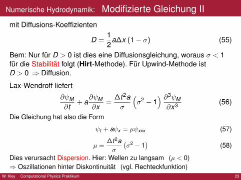
Numerische Hydrodynamik: Modifizierte Gleichung II

mit Diffusions-Koeffizienten

D =12

a∆x (1− σ) (55)

Bem: Nur fur D > 0 ist dies eine Diffusionsgleichung, woraus σ < 1fur die Stabilitat folgt (Hirt-Methode). Fur Upwind-Methode istD > 0 ⇒ Diffusion.

Lax-Wendroff liefert

∂ψM

∂t+ a

∂ψM

∂x=

∆t2aσ

(σ2 − 1

) ∂3ψM

∂x3 (56)

Die Gleichung hat also die Form

ψt + aψx = µψxxx (57)

µ =∆t2aσ

(σ2 − 1

)(58)

Dies verursacht Dispersion. Hier: Wellen zu langsam (µ < 0)⇒ Oszillationen hinter Diskontinuitat (vgl. Rechteckfunktion)


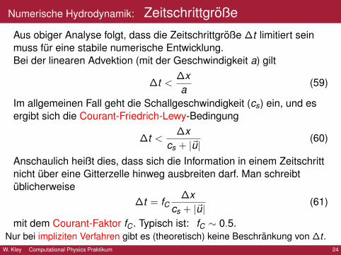
Numerische Hydrodynamik: Zeitschrittgroße

Aus obiger Analyse folgt, dass die Zeitschrittgroße ∆t limitiert seinmuss fur eine stabile numerische Entwicklung.Bei der linearen Advektion (mit der Geschwindigkeit a) gilt

∆t <∆xa

(59)

Im allgemeinen Fall geht die Schallgeschwindigkeit (cs) ein, und esergibt sich die Courant-Friedrich-Lewy-Bedingung

∆t <∆x

cs + |~u|(60)

Anschaulich heißt dies, dass sich die Information in einem Zeitschrittnicht uber eine Gitterzelle hinweg ausbreiten darf. Man schreibtublicherweise

∆t = fC∆x

cs + |~u|(61)

mit dem Courant-Faktor fC . Typisch ist: fC ∼ 0.5.Nur bei impliziten Verfahren gibt es (theoretisch) keine Beschrankung von ∆t .


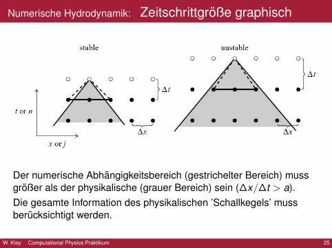
Numerische Hydrodynamik: Zeitschrittgroße graphisch

Der numerische Abhangigkeitsbereich (gestrichelter Bereich) mussgroßer als der physikalische (grauer Bereich) sein (∆x/∆t > a).Die gesamte Information des physikalischen ’Schallkegels’ mussberucksichtigt werden.


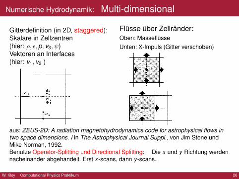
Numerische Hydrodynamik: Multi-dimensional

Gitterdefinition (in 2D, staggered):Skalare in Zellzentren(hier: ρ, ε,p, v3, ψ)Vektoren an Interfaces(hier: v1, v2 )

Flusse uber Zellrander:Oben: MasseflusseUnten: X-Impuls (Gitter verschoben)

aus: ZEUS-2D: A radiation magnetohydrodynamics code for astrophysical flows intwo space dimensions. I in The Astrophysical Journal Suppl., von Jim Stone undMike Norman, 1992.Benutze Operator-Splitting und Directional Splitting: Die x und y Richtung werdennacheinander abgehandelt. Erst x-scans, dann y -scans.


Numerische Hydrodynamik: ZusammenfassungNumerische Methoden sollten Erhaltungseigenschaften wiedergeben.

Gleichungen in Erhaltungsform schreibenNumerische Methoden sollten Welleneigenschaften wiedergeben.

Shock-Capturing Methoden, Riemann-LoserNumerische Methoden mussen Diskontinuitaten unter Kontrolle halten.

Brauche dazu Diffusion (⇒ Stabilitat)entweder explizit (kunstliche Viskositat) oder intrinsisch (durch Verfahren)

Numerische Methoden sollten genau seinmind. 2. Ordnung in Zeit und Raum

Frei verfugbare Codes:ZEUS: http://www.astro.princeton.edu/~jstone/zeus.html

klassischer Upwind-Code, zweiter Ordnung, staggered grid, RMHDATHENA: https://trac.princeton.edu/Athena/

Nachfolger von ZEUS: Riemann Loser, zentriertes Gitter, MHDNIRVANA: http://nirvana-code.aip.de/

3D, AMR, Finite Volume Code, MHDPLUTO: http://plutocode.ph.unito.it/

3D, relativistisch, Riemann-Loser/Finite Volume, MHDGADGET: http://www.mpa-garching.mpg.de/galform/gadget/

SPH-Code, Tree-Code, Eigengrav. (Galaxien)W. Kley Computational Physics Praktikum 27

http://www.astro.princeton.edu/~jstone/zeus.html

https://trac.princeton.edu/Athena/

http://nirvana-code.aip.de/

http://plutocode.ph.unito.it/

http://www.mpa-garching.mpg.de/galform/gadget/

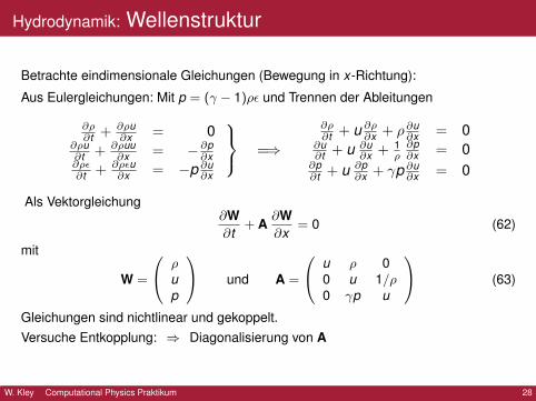
Hydrodynamik: Wellenstruktur

Betrachte eindimensionale Gleichungen (Bewegung in x-Richtung):

Aus Eulergleichungen: Mit p = (γ − 1)ρε und Trennen der Ableitungen

∂ρ∂t + ∂ρu

∂x = 0∂ρu∂t + ∂ρuu

∂x = −∂p∂x

∂ρε∂t + ∂ρεu

∂x = −p ∂u∂x

=⇒

∂ρ∂t + u ∂ρ∂x + ρ∂u

∂x = 0∂u∂t + u ∂u

∂x + 1ρ∂p∂x = 0

∂p∂t + u ∂p

∂x + γp ∂u∂x = 0

Als Vektorgleichung∂W∂t

+ A∂W∂x

= 0 (62)

mit

W =

ρup

und A =

u ρ 00 u 1/ρ0 γp u

(63)

Gleichungen sind nichtlinear und gekoppelt.Versuche Entkopplung: ⇒ Diagonalisierung von A


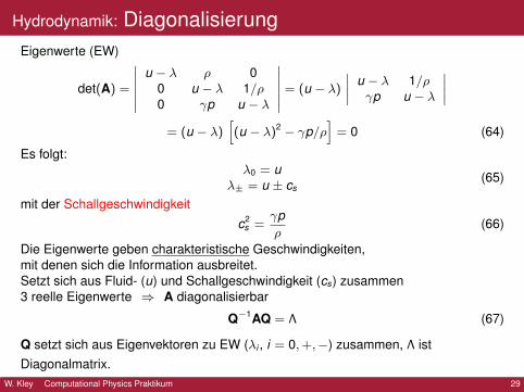
Hydrodynamik: DiagonalisierungEigenwerte (EW)

det(A) =

∣∣∣∣∣∣u − λ ρ 0

0 u − λ 1/ρ0 γp u − λ

∣∣∣∣∣∣ = (u − λ)

∣∣∣∣ u − λ 1/ργp u − λ

∣∣∣∣= (u − λ)

[(u − λ)2 − γp/ρ

]= 0 (64)

Es folgt:λ0 = u

λ± = u ± cs(65)

mit der Schallgeschwindigkeitc2

s =γpρ

(66)

Die Eigenwerte geben charakteristische Geschwindigkeiten,mit denen sich die Information ausbreitet.Setzt sich aus Fluid- (u) und Schallgeschwindigkeit (cs) zusammen3 reelle Eigenwerte ⇒ A diagonalisierbar

Q−1AQ = Λ (67)

Q setzt sich aus Eigenvektoren zu EW (λi , i = 0,+,−) zusammen, Λ istDiagonalmatrix.


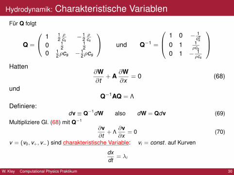
Hydrodynamik: Charakteristische VariablenFur Q folgt

Q =

1 12ρcs

− 12ρcs

0 12

12

0 12ρcs − 1

2ρcs

und Q−1 =

1 0 − 1c2

s

0 1 1ρcs

0 1 − 1ρcs

Hatten

∂W∂t

+ A∂W∂x

= 0 (68)

undQ−1AQ = Λ

Definiere:dv ≡ Q−1dW also dW = Qdv (69)

Multipliziere Gl. (68) mit Q−1

∂v∂t

+ Λ∂v∂x

= 0 (70)

v = (v0, v+, v−) sind charakteristische Variable: vi = const . auf Kurven

dxdt

= λi


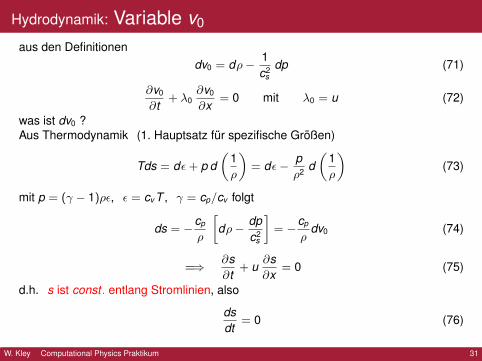
Hydrodynamik: Variable v0

aus den Definitionendv0 = dρ− 1

c2s

dp (71)

∂v0

∂t+ λ0

∂v0

∂x= 0 mit λ0 = u (72)

was ist dv0 ?Aus Thermodynamik (1. Hauptsatz fur spezifische Großen)

Tds = dε+ p d(

1ρ

)= dε− p

ρ2 d(

1ρ

)(73)

mit p = (γ − 1)ρε, ε = cv T , γ = cp/cv folgt

ds = −cp

ρ

[dρ− dp

c2s

]= −cp

ρdv0 (74)

=⇒ ∂s∂t

+ u∂s∂x

= 0 (75)

d.h. s ist const . entlang Stromlinien, also

dsdt

= 0 (76)


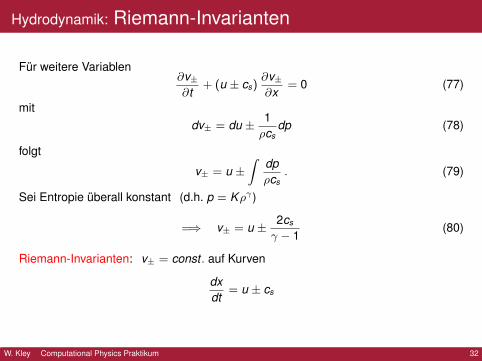
Hydrodynamik: Riemann-Invarianten

Fur weitere Variablen∂v±

∂t+ (u ± cs)

∂v±

∂x= 0 (77)

mitdv± = du ± 1

ρcsdp (78)

folgt

v± = u ±∫

dpρcs

. (79)

Sei Entropie uberall konstant (d.h. p = Kργ)

=⇒ v± = u ± 2cs

γ − 1(80)

Riemann-Invarianten: v± = const . auf Kurven

dxdt

= u ± cs


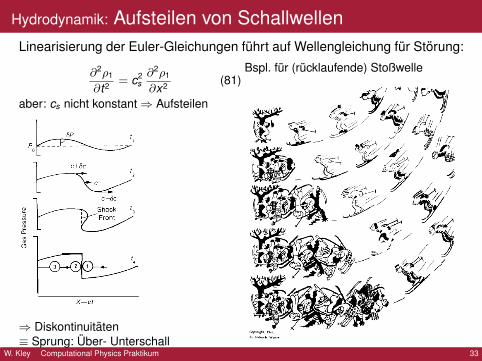
Hydrodynamik: Aufsteilen von SchallwellenLinearisierung der Euler-Gleichungen fuhrt auf Wellengleichung fur Storung:

∂2ρ1

∂t2 = c2s∂2ρ1

∂x2 (81)

aber: cs nicht konstant⇒ Aufsteilen

⇒ Diskontinuitaten≡ Sprung: Uber- Unterschall

Bspl. fur (rucklaufende) Stoßwelle


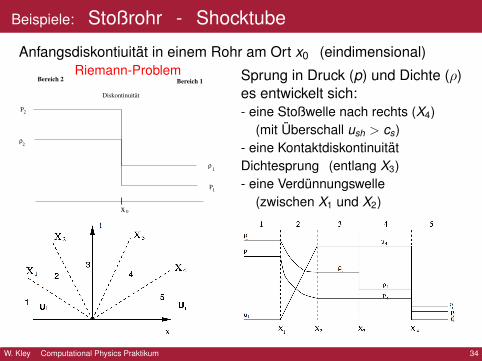
Beispiele: Stoßrohr - Shocktube

Anfangsdiskontiuitat in einem Rohr am Ort x0 (eindimensional)Riemann-Problem

0

P

P

ρ

ρ

2

2

1

1

Bereich 1

Diskontinuität

Bereich 2

x

Sprung in Druck (p) und Dichte (ρ)es entwickelt sich:- eine Stoßwelle nach rechts (X4)

(mit Uberschall ush > cs)- eine KontaktdiskontinuitatDichtesprung (entlang X3)- eine Verdunnungswelle

(zwischen X1 und X2)


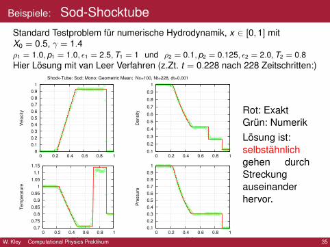
Beispiele: Sod-ShocktubeStandard Testproblem fur numerische Hydrodynamik, x ∈ [0,1] mitX0 = 0.5, γ = 1.4ρ1 = 1.0, p1 = 1.0, ε1 = 2.5,T1 = 1 und ρ2 = 0.1, p2 = 0.125, ε2 = 2.0,T2 = 0.8Hier Losung mit van Leer Verfahren (z.Zt. t = 0.228 nach 228 Zeitschritten:)

0

0.1

0.2

0.3

0.4

0.5

0.6

0.7

0.8

0.9

1

0 0.2 0.4 0.6 0.8 1

Ve

loci

ty

Shock-Tube: Sod; Mono: Geometric Mean; Nx=100, Nt=228, dt=0.001

0.1

0.2

0.3

0.4

0.5

0.6

0.7

0.8

0.9

1

0 0.2 0.4 0.6 0.8 1

De

nsi

ty

0.7

0.75

0.8

0.85

0.9

0.95

1

1.05

1.1

1.15

0 0.2 0.4 0.6 0.8 1

Te

mp

era

ture

X-Axis

0.1

0.2

0.3

0.4

0.5

0.6

0.7

0.8

0.9

1

0 0.2 0.4 0.6 0.8 1

Pre

ssu

re

X-Axis

Rot: ExaktGrun: NumerikLosung ist:selbstahnlichgehen durchStreckungauseinanderhervor.


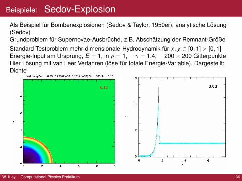
Beispiele: Sedov-ExplosionAls Beispiel fur Bombenexplosionen (Sedov & Taylor, 1950er), analytische Losung(Sedov)Grundproblem fur Supernovae-Ausbruche, z.B. Abschatzung der Remnant-GroßeStandard Testproblem mehr-dimensionale Hydrodynamik fur x , y ∈ [0, 1]× [0, 1]Energie-Input am Ursprung, E = 1, in ρ = 1, γ = 1.4, 200× 200 GitterpunkteHier Losung mit van Leer Verfahren (lose fur totale Energie-Variable). Dargestellt:Dichte


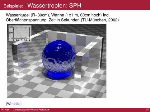
Beispiele: Wassertropfen: SPHWasserkugel (R=30cm), Wanne (1x1 m, 60cm hoch) Incl.Oberflachenspannung, Zeit in Sekunden (TU-Munchen, 2002)

(Website)W. Kley Computational Physics Praktikum 37

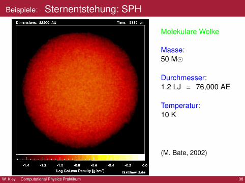
http://www.t35.physik.tu-muenchen.de/lectures/sph.html

Beispiele: Sternentstehung: SPH

Molekulare Wolke

Masse:50 M�

Durchmesser:1.2 LJ = 76,000 AE

Temperatur:10 K

(M. Bate, 2002)


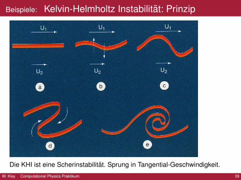
Beispiele: Kelvin-Helmholtz Instabilitat: Prinzip

Die KHI ist eine Scherinstabilitat. Sprung in Tangential-Geschwindigkeit.


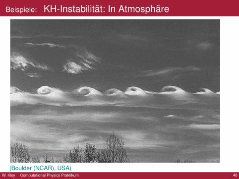
Beispiele: KH-Instabilitat: In Atmosphare

(Boulder (NCAR), USA)W. Kley Computational Physics Praktikum 40

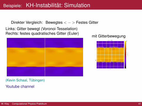
Beispiele: KH-Instabilitat: Simulation

Direkter Vergleich: Bewegtes < − > Festes Gitter

Links: Gitter bewegt (Voronoi-Tesselation)Rechts: festes quadratisches Gitter (Euler)

mit Gitterbewegung

(Kevin Schaal, Tubingen)

Youtube channel


https://www.youtube.com/channel/UC6CZ_Bcyql1kfHZvx9W85mA

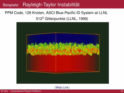
Beispiele: Rayleigh-Taylor Instabilitat

PPM Code, 128 Knoten, ASCI Blue-Pacific ID System at LLNL

5123 Gitterpunkte (LLNL, 1999)

(Web-Link)W. Kley Computational Physics Praktikum 42

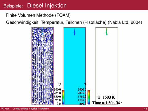
https://computation.llnl.gov/casc/asciturb/simulations.shtml

Beispiele: Diesel Injektion

Finite Volumen Methode (FOAM)

Geschwindigkeit, Temperatur, Teilchen (+Isoflache) (Nabla Ltd, 2004)


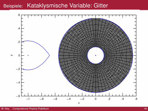
Beispiele: Kataklysmische Variable: Gitter

−1 −.8 −.6 −.4 −.2 0 .2 .4 .6−.6

−.4

−.2

0

.2

.4

.6

x

y


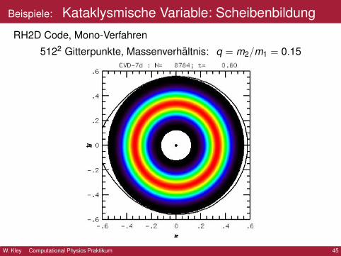
Beispiele: Kataklysmische Variable: Scheibenbildung

RH2D Code, Mono-Verfahren

5122 Gitterpunkte, Massenverhaltnis: q = m2/m1 = 0.15


Computational Physics Praktikum: Numerische Hydrodynamikkley/... · Computational Physics...

Documents

Transcript of Computational Physics Praktikum: Numerische Hydrodynamikkley/... · Computational Physics...