Dra

ftComputation of frequency responses of PDEsin Chebfun

Mihailo Jovanovicwww.umn.edu/∼mihailo

joint work with:Binh K. Lieu

2012 SIAM Annual Meeting

Dra

ft

M. JOVANOVIC, UMN 1

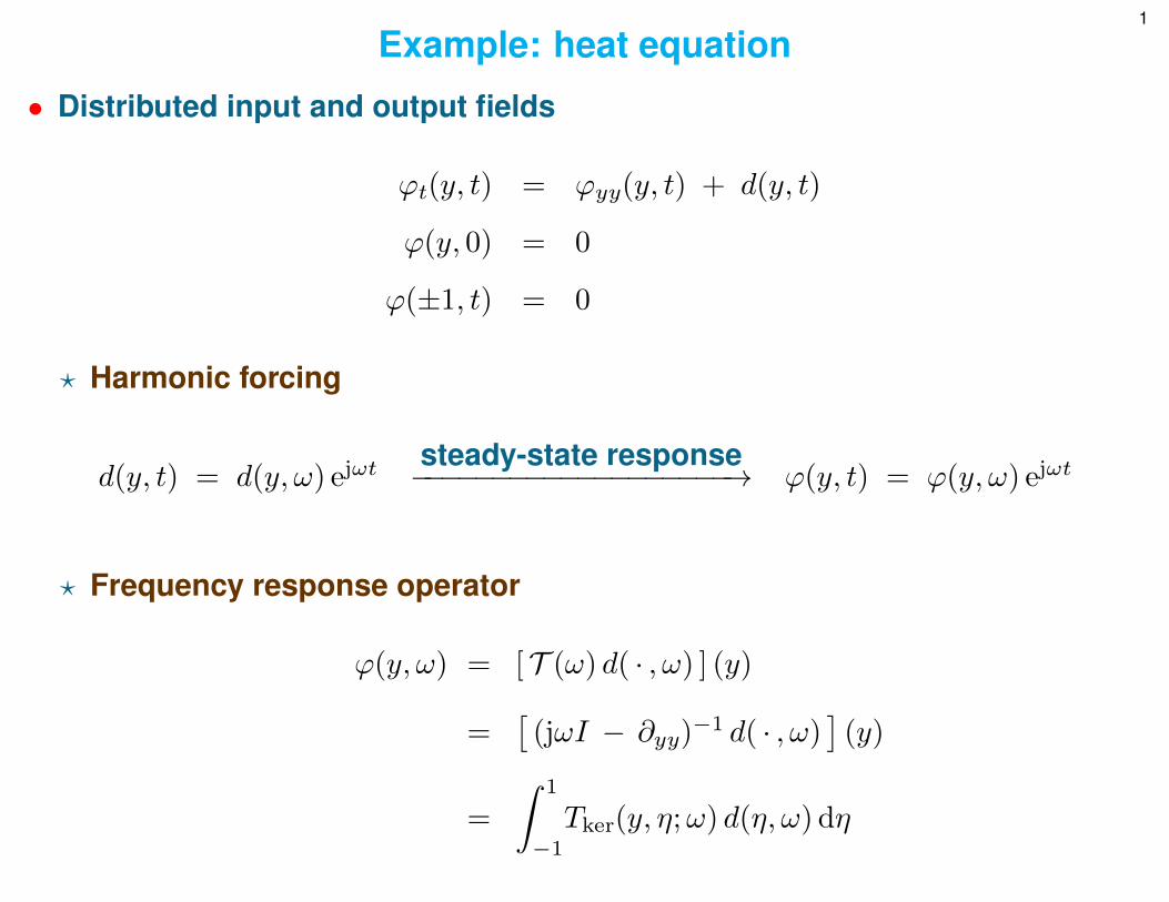
Example: heat equation

• Distributed input and output fields

ϕt(y, t) = ϕyy(y, t) + d(y, t)

ϕ(y, 0) = 0

ϕ(±1, t) = 0

? Harmonic forcing

d(y, t) = d(y, ω) ejωtsteady-state response−−−−−−−−−−−−−−−−−−−→ ϕ(y, t) = ϕ(y, ω) ejωt

? Frequency response operator

ϕ(y, ω) = [ T (ω) d( · , ω) ] (y)

=[

(jωI − ∂yy)−1 d( · , ω)

](y)

=

∫ 1

−1Tker(y, η;ω) d(η, ω) dη

Dra

ft

M. JOVANOVIC, UMN 2

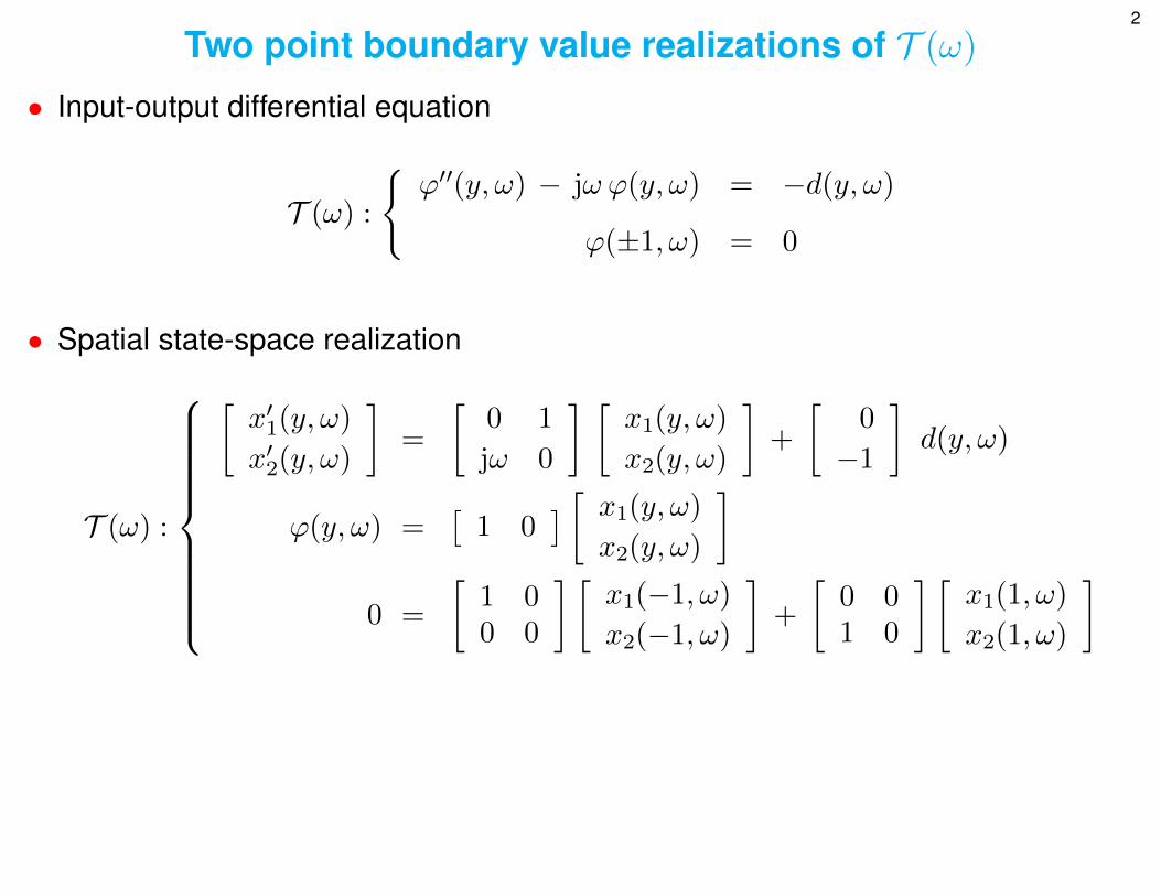
Two point boundary value realizations of T (ω)

• Input-output differential equation

T (ω) :

{ϕ′′(y, ω) − jω ϕ(y, ω) = −d(y, ω)

ϕ(±1, ω) = 0

• Spatial state-space realization

T (ω) :

[x′1(y, ω)

x′2(y, ω)

]=

[0 1

jω 0

] [x1(y, ω)

x2(y, ω)

]+

[0

−1

]d(y, ω)

ϕ(y, ω) =[

1 0] [ x1(y, ω)

x2(y, ω)

]0 =

[1 00 0

] [x1(−1, ω)

x2(−1, ω)

]+

[0 01 0

] [x1(1, ω)

x2(1, ω)

]

Dra

ft

M. JOVANOVIC, UMN 3

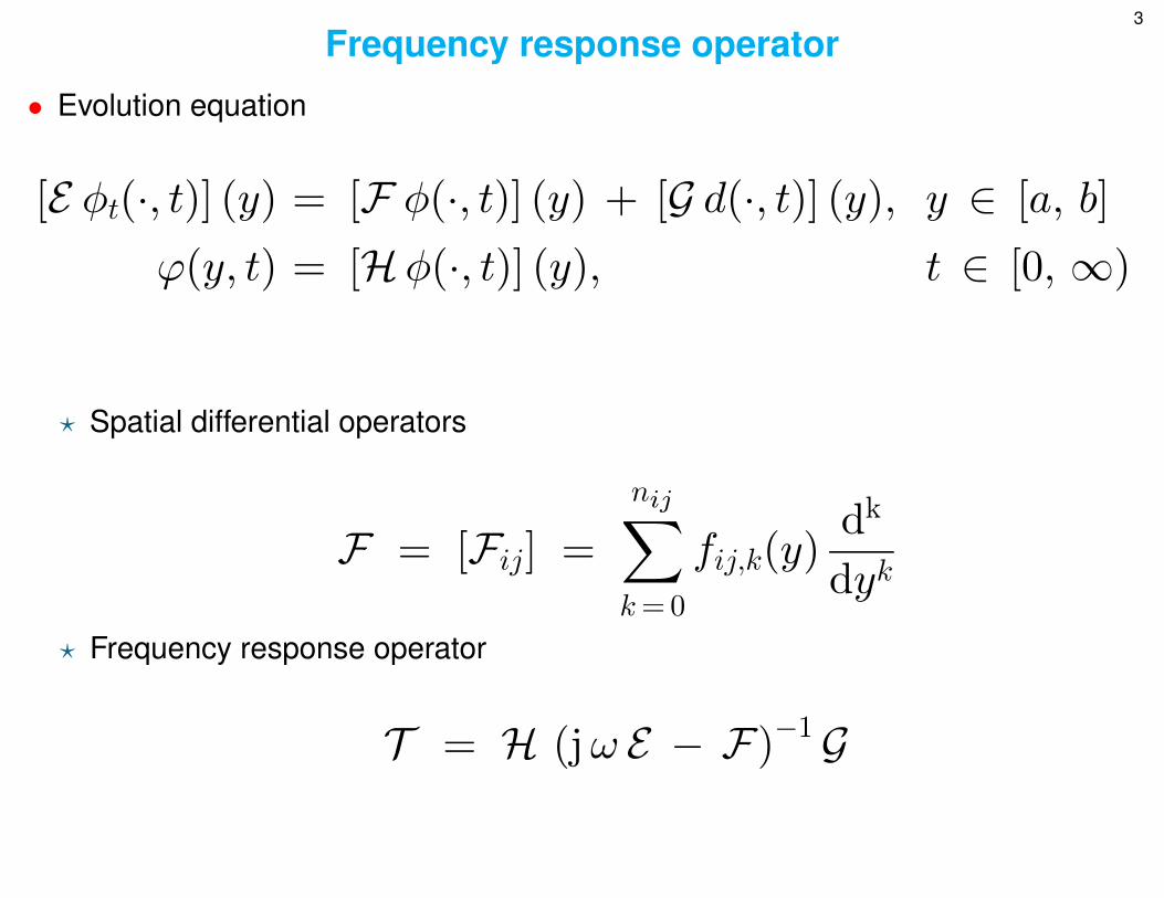
Frequency response operator

• Evolution equation

[E φt(·, t)] (y) = [F φ(·, t)] (y) + [G d(·, t)] (y), y ∈ [a, b]

ϕ(y, t) = [Hφ(·, t)] (y), t ∈ [0, ∞)

? Spatial differential operators

F = [Fij] =

nij∑k= 0

fij,k(y)dk

dyk

? Frequency response operator

T = H (jω E − F)−1 G

Dra

ft

M. JOVANOVIC, UMN 4

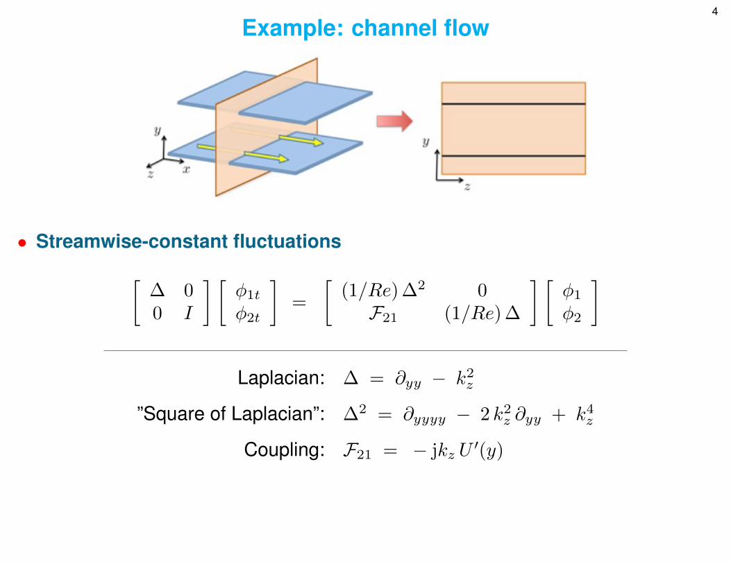
Example: channel flow

• Streamwise-constant fluctuations[∆ 00 I

] [φ1tφ2t

]=

[(1/Re) ∆2 0F21 (1/Re) ∆

] [φ1φ2

]

Laplacian: ∆ = ∂yy − k2z

”Square of Laplacian”: ∆2 = ∂yyyy − 2 k2z ∂yy + k4z

Coupling: F21 = − jkz U′(y)

Dra

ft

M. JOVANOVIC, UMN 5

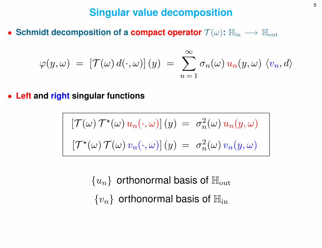
Singular value decomposition

• Schmidt decomposition of a compact operator T (ω): Hin −→ Hout

ϕ(y, ω) = [T (ω) d(·, ω)] (y) =

∞∑n=1

σn(ω)un(y, ω) 〈vn, d〉

• Left and right singular functions

[T (ω) T ?(ω)un(·, ω)] (y) = σ2n(ω)un(y, ω)

[T ?(ω) T (ω) vn(·, ω)] (y) = σ2n(ω) vn(y, ω)

{un} orthonormal basis of Hout

{vn} orthonormal basis of Hin

Dra

ft

M. JOVANOVIC, UMN 6

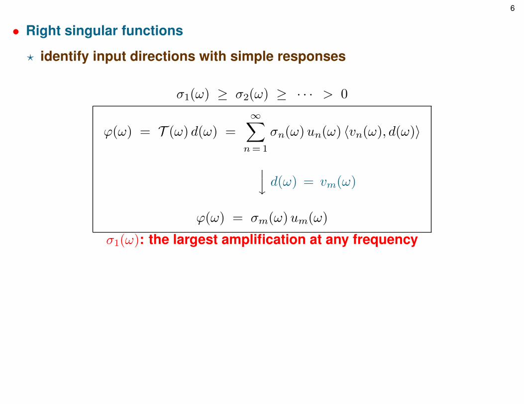
• Right singular functions

? identify input directions with simple responses

σ1(ω) ≥ σ2(ω) ≥ · · · > 0

ϕ(ω) = T (ω) d(ω) =

∞∑n=1

σn(ω)un(ω) 〈vn(ω), d(ω)〉

y d(ω) = vm(ω)

ϕ(ω) = σm(ω)um(ω)

σ1(ω): the largest amplification at any frequency

Dra

ft

M. JOVANOVIC, UMN 7

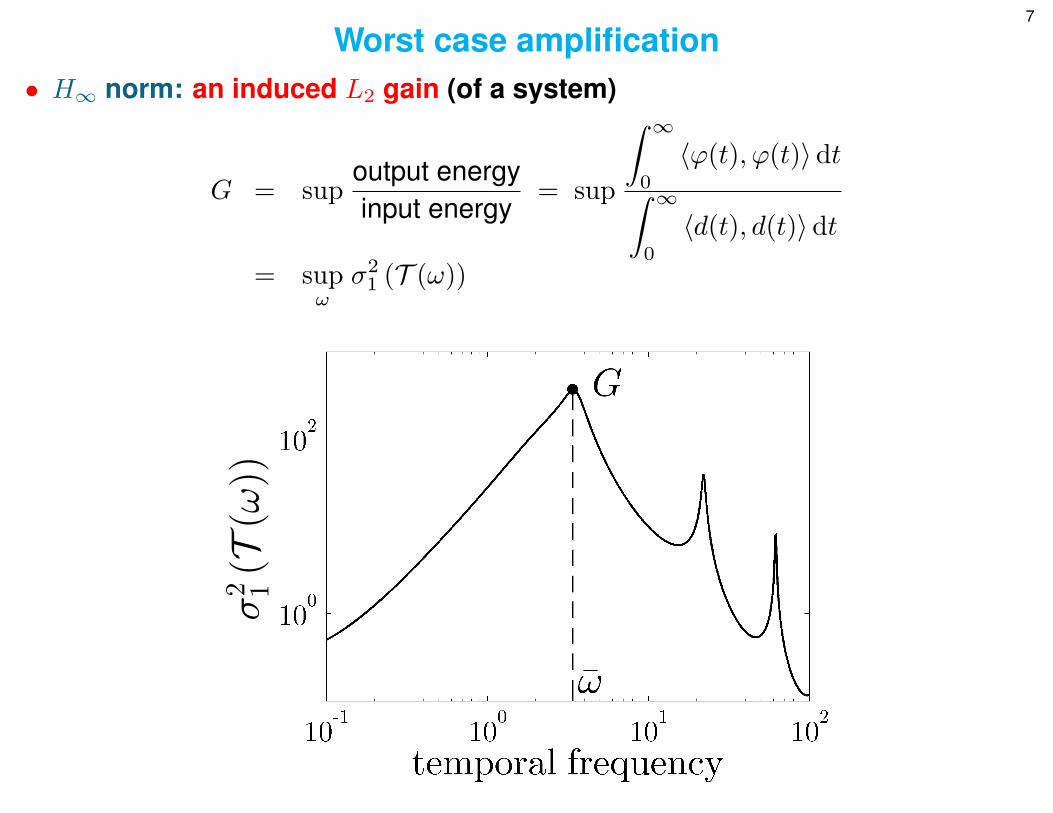
Worst case amplification• H∞ norm: an induced L2 gain (of a system)

G = supoutput energyinput energy

= sup

∫ ∞0

〈ϕ(t), ϕ(t)〉dt∫ ∞0

〈d(t), d(t)〉dt

= supωσ21 (T (ω))

σ2 1(T

(ω))

Dra

ft

M. JOVANOVIC, UMN 8

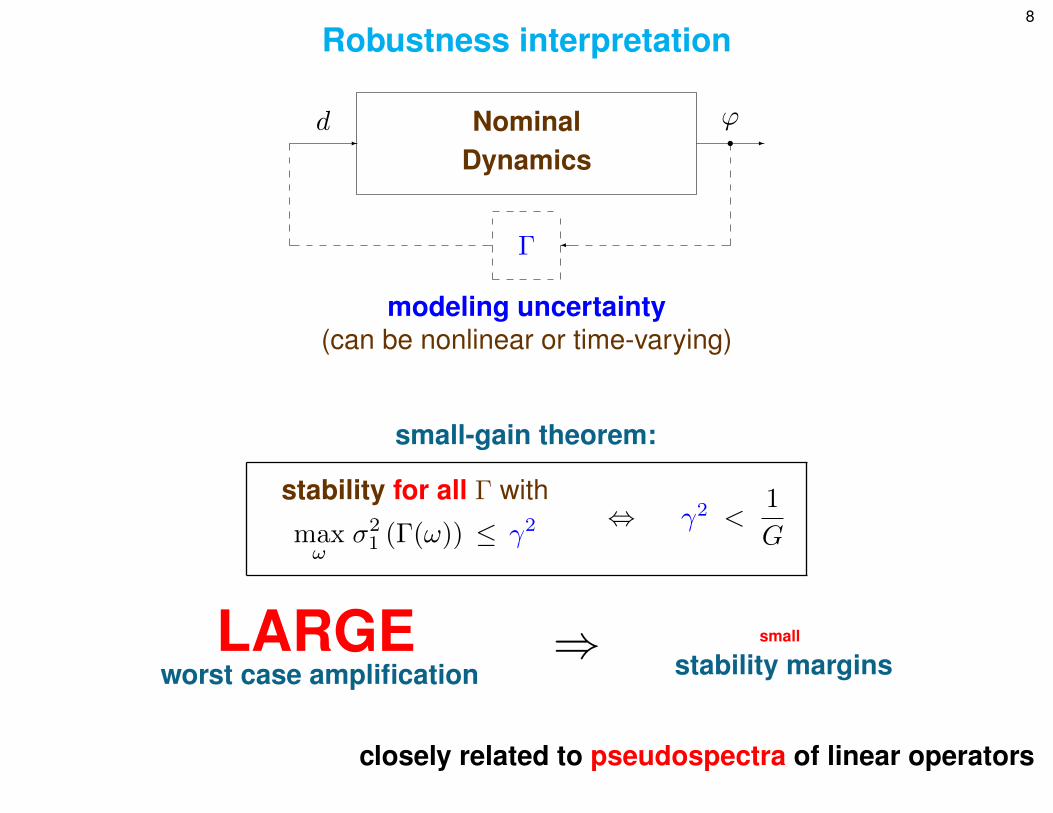
Robustness interpretation

-d Nominal

Dynamicss -

ϕ

�Γ

modeling uncertainty(can be nonlinear or time-varying)

small-gain theorem:

stability for all Γ with

maxω

σ21 (Γ(ω)) ≤ γ2

⇔ γ2 <1

G

LARGEworst case amplification

⇒ small

stability margins

closely related to pseudospectra of linear operators

Dra

ft

M. JOVANOVIC, UMN 9

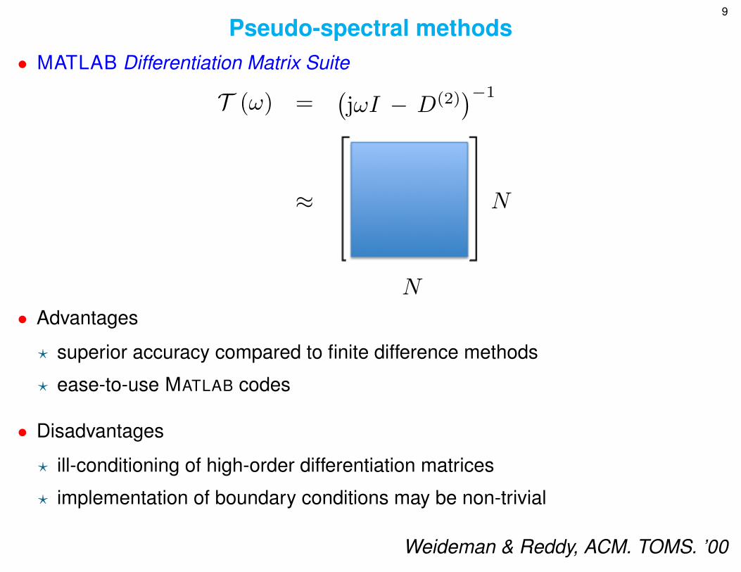
Pseudo-spectral methods• MATLAB Differentiation Matrix Suite

T (ω) =(jωI − D(2)

)−1

≈ N

N

• Advantages

? superior accuracy compared to finite difference methods

? ease-to-use MATLAB codes

• Disadvantages

? ill-conditioning of high-order differentiation matrices

? implementation of boundary conditions may be non-trivial

Weideman & Reddy, ACM. TOMS. ’00

Dra

ft

M. JOVANOVIC, UMN 10

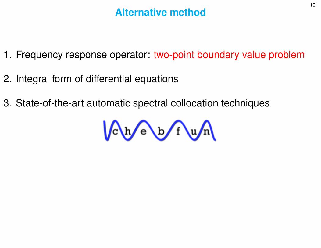
Alternative method

1. Frequency response operator: two-point boundary value problem

2. Integral form of differential equations

3. State-of-the-art automatic spectral collocation techniques

Dra

ft

M. JOVANOVIC, UMN 11

Advantages of Chebfun

• Superior accuracy compared to currently available schemes

• Avoids ill-conditioning of high-order differentiation matrices

• Incorporates a wide range of boundary conditions

• Easy-to-use MATLAB codes

Lieu & Jovanovic“Computation of frequency responses of linear time-invariant PDEs on a compactinterval”, submitted to J. Comput. Phys., 2011Also arXiv:1112.0579v1

Dra

ft

M. JOVANOVIC, UMN 12

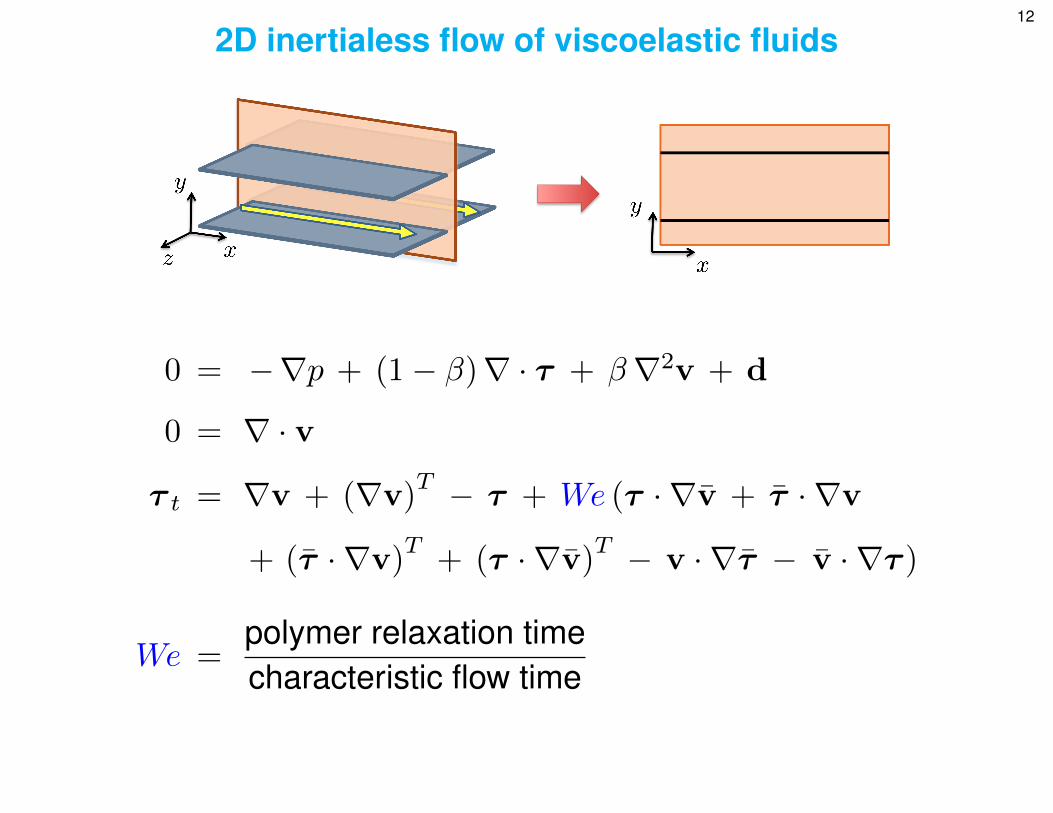
2D inertialess flow of viscoelastic fluids

0 = −∇p + (1− β)∇ · τ + β∇2v + d

0 = ∇ · v

τ t = ∇v + (∇v)T − τ + We (τ · ∇v + τ · ∇v

+ (τ · ∇v)T

+ (τ · ∇v)T − v · ∇τ − v · ∇τ )

We =polymer relaxation timecharacteristic flow time

Dra

ft

M. JOVANOVIC, UMN 13

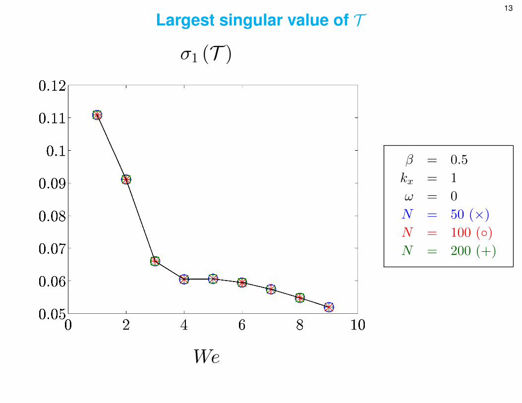
Largest singular value of T

σ1 (T )

We

β = 0.5

kx = 1

ω = 0

N = 50 (×)

N = 100 (◦)N = 200 (+)

Dra

ft

M. JOVANOVIC, UMN 14

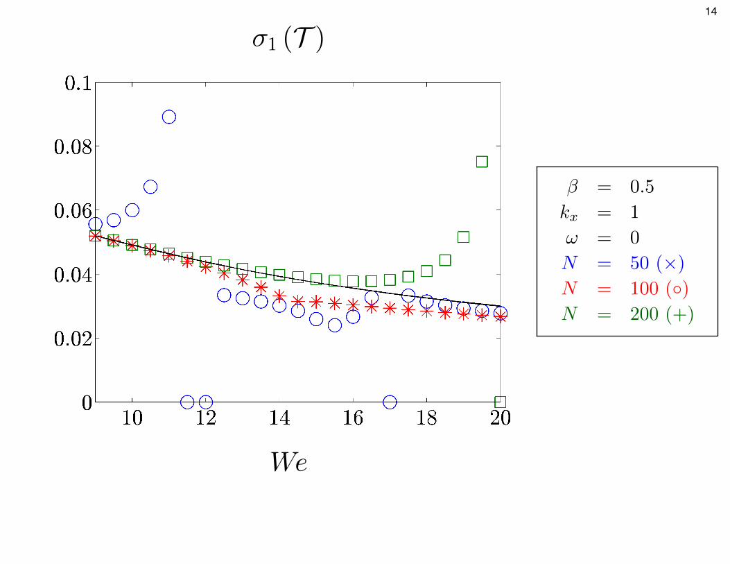
σ1 (T )

We

β = 0.5

kx = 1

ω = 0

N = 50 (×)

N = 100 (◦)N = 200 (+)

Dra

ft

M. JOVANOVIC, UMN 15

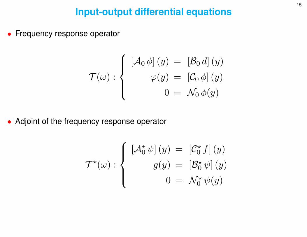
Input-output differential equations

• Frequency response operator

T (ω) :

[A0 φ] (y) = [B0 d] (y)

ϕ(y) = [C0 φ] (y)

0 = N0 φ(y)

• Adjoint of the frequency response operator

T ?(ω) :

[A?0 ψ] (y) = [C?0 f ] (y)

g(y) = [B?0 ψ] (y)

0 = N ?0 ψ(y)

Dra

ft

M. JOVANOVIC, UMN 16

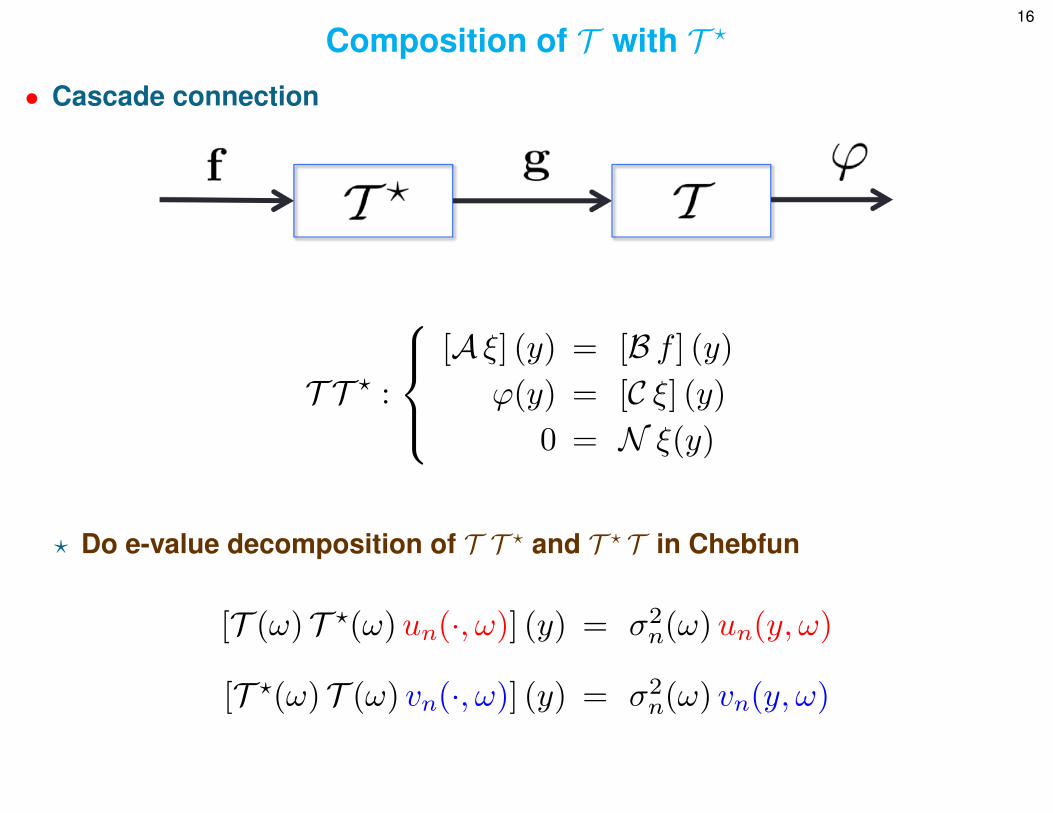
Composition of T with T ?

• Cascade connection

T T ? :

[A ξ] (y) = [B f ] (y)

ϕ(y) = [C ξ] (y)

0 = N ξ(y)

? Do e-value decomposition of T T ? and T ? T in Chebfun

[T (ω) T ?(ω)un(·, ω)] (y) = σ2n(ω)un(y, ω)

[T ?(ω) T (ω) vn(·, ω)] (y) = σ2n(ω) vn(y, ω)

Dra

ft

M. JOVANOVIC, UMN 17

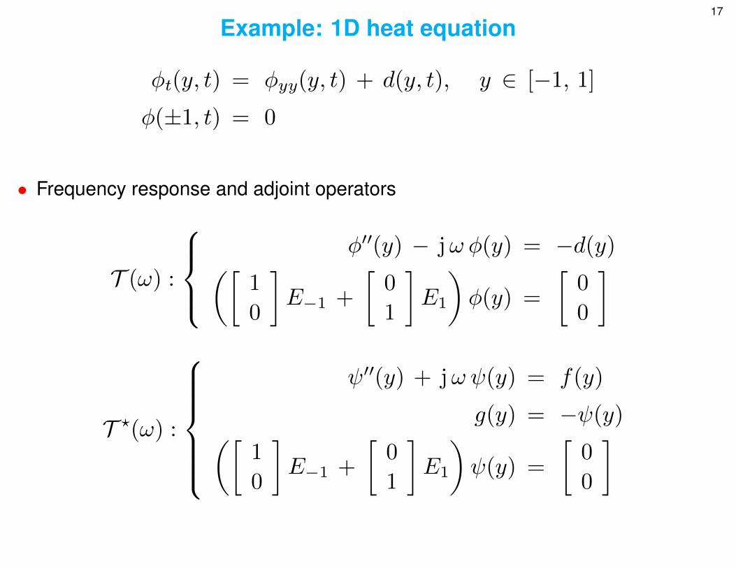
Example: 1D heat equation

φt(y, t) = φyy(y, t) + d(y, t), y ∈ [−1, 1]

φ(±1, t) = 0

• Frequency response and adjoint operators

T (ω) :

φ′′(y) − jω φ(y) = −d(y)([

1

0

]E−1 +

[0

1

]E1

)φ(y) =

[0

0

]

T ?(ω) :

ψ′′(y) + jω ψ(y) = f(y)

g(y) = −ψ(y)([1

0

]E−1 +

[0

1

]E1

)ψ(y) =

[0

0

]

Dra

ft

M. JOVANOVIC, UMN 18

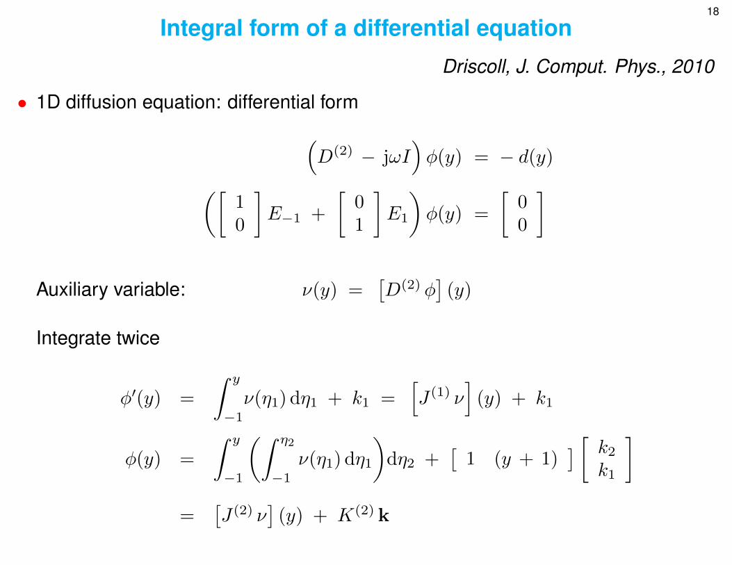
Integral form of a differential equation

Driscoll, J. Comput. Phys., 2010

• 1D diffusion equation: differential form(D(2) − jωI

)φ(y) = − d(y)([

10

]E−1 +

[01

]E1

)φ(y) =

[00

]

Auxiliary variable: ν(y) =[D(2) φ

](y)

Integrate twice

φ′(y) =

∫ y

−1ν(η1) dη1 + k1 =

[J (1) ν

](y) + k1

φ(y) =

∫ y

−1

(∫ η2

−1ν(η1) dη1

)dη2 +

[1 (y + 1)

] [ k2k1

]=

[J (2) ν

](y) + K(2) k

Dra

ft

M. JOVANOVIC, UMN 19

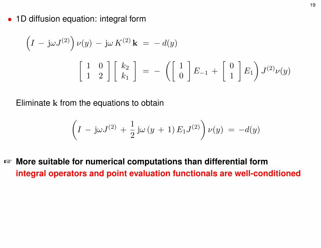
• 1D diffusion equation: integral form(I − jωJ (2)

)ν(y) − jωK(2) k = − d(y)

[1 01 2

] [k2k1

]= −

([10

]E−1 +

[01

]E1

)J (2)ν(y)

Eliminate k from the equations to obtain(I − jωJ (2) +

1

2jω (y + 1)E1J

(2)

)ν(y) = −d(y)

+ More suitable for numerical computations than differential formintegral operators and point evaluation functionals are well-conditioned

Dra

ft

M. JOVANOVIC, UMN 20

Online resources

• Chebfun

http://www2.maths.ox.ac.uk/chebfun/

Google: “chebfun”

• Computing frequency responses of PDEs

http://www.umn.edu/∼mihailo/software/chebfun-svd/

Google: “frequency responses pde”

Dra

ft

M. JOVANOVIC, UMN 21

Summary

• method for computing frequency responses of PDEs

• easy-to-use mini-toolbox in MATLAB

? enabling tool: Chebfun

• two major advantages over currently available schemes

? avoids ill-conditioning of high-order differentiation matrices

? easy implementation of boundary conditions

Dra

ft

M. JOVANOVIC, UMN 22

Acknowledgments

TEAM:

Binh Lieu

SUPPORT:

NSF CAREER Award CMMI-06-44793

SOFTWARE:

http://www.umn.edu/∼mihailo/software/chebfun-svd/