Computability Theory - Zur Startseite · They have provided the foundation of computability ......
118
Computability Theory Karl-Heinz Zimmermann
Transcript of Computability Theory - Zur Startseite · They have provided the foundation of computability ......
Computability Theory
Karl-Heinz Zimmermann


Computability Theory

Karl-Heinz Zimmermann
Computability Theory
Hamburg University of Technology
Prof. Dr. Karl-Heinz ZimmermannHamburg University of Technology21071 HamburgGermany
This monograph is listed in the GBV database and the TUHH library.
All rights reservedc©second edition, 2012, by Karl-Heinz Zimmermann, authorc©first edition, 2011, by Karl-Heinz Zimmermann, autor
urn:nbn:de:gbv:830-tubdok-11600

For Gela and Eileen

VI
Preface to the 2nd Edition
Why do we need a formalization of the notion of algorithm or effective computation? In order to showthat a specific problem is algorithmically solvable, it is sufficient to provide an algorithm that solves itin a sufficiently precise manner. However, in order to prove that a problem is in principle not solvableby an algorithm, a rigorous formalism is necessary that allows mathematical proofs. The need for sucha formalism became apparent in the studies of David Hilbert (1900) on the foundations of mathematicsand Kurt Godel (1931) on the incompleteness of elementary arithmetic.
The first investigations in the field were conducted by the logicians Alonzo Church, Stephen Kleene,Emil Post, and Alan Turing in the early 1930s. They have provided the foundation of computabilitytheory as a branch of theoretical computer science. The fundamental results established Turing com-putability as the correct formalization of the informal idea of effective calculation. The results have ledto Church’s thesis stating that ”everything computable is computable by a Turing machine”. The the-ory of computability has grown rapidly from its beginning. Its questions and methods are penetratingmany other mathematical disciplines. Today, computability theory provides an important theoreticalbackground for logicians, pure mathematicians, and computer scientists. Many mathematical problemsare known to be undecidable such as the word problem for groups, the halting problem, and Hilbert’stenth problem.
This book is a development of class notes for a two-hour lecture including a one-hour lab held forsecond-year Bachelor students of Computer Science at the Hamburg University of Technology duringthe last two years. The course aims to present the basic results of computability theory, includingmathematical models of computability, primitive recursive and partial recursive functions, Ackermann’sfunction, Godel numbering, universal functions, smn theorem, Kleene’s normal form, undecidable sets,theorems of Rice, and word problems. The manuscript has partly grown out of notes taken by theauthor during his studies at the University of Erlangen-Nuremberg. I would like to thank again myteachers Martin Becker† and Volker Strehl for giving inspiring lectures in this field.
The second edition contains minor changes. In particular, the section on Godel numbering has beenrewritten and a glossary of terms has been added.
VIII Preface to the 2nd Edition
Finally, I would like to express my thanks to Ralf Moller for valuable comments. I am also gratefulto Mahwish Saleemi for conducting the lab and to Wolfgang Brandt for valuable technical support.Moreover, I would like to thank my students for their attention, their stimulating questions, and theirdedicated work.
Hamburg, July 2012 Karl-Heinz Zimmermann
Mathematical Notation IX
Mathematical Notation
General notation
N0 set of natural numbersN set of natural number without 0Z set of integersΣ∗ set of words over ΣΣ+ set of non-empty words over ΣF class of partial functionsP class of primitive recursive functionsR class of partial recursive functionsT class of recursive functionsFURM class of URM computable functionsTURM class of total URM computable functionsFLOOP class of LOOP computable functionsPLOOP class of LOOP programsFLOOP−n class of LOOP-n computable functionsPLOOP−n class of LOOP-n programsFGOTO class of GOTO computable functionsPGOTO class of GOTO programsPSGOTO class of SGOTO programsTTuring class of Turing computable functions
Chapter 1
Ω state set of URME(Ω) set of state transitionsdomf domain of a functionranf range of a function− conditional decrementsgn sign functioncsg cosign functionf∗n iteration of f w.r.t. nth registerAσ incrementSσ conditional decrement(P )σ iteration of a programP ;Q composition of programs|P | state transition function of a program‖P‖k,m function of a programαk load functionβm result function
X Mathematical Notation
R(i; j1, . . . , jk) reload programC(i; j1, . . . , jk) copy program
Chapter 2
ν successor function
c(n)0 n-ary zero function
π(n)k n-ary projection function
pr(g, h) primitive recursiong(h1, . . . , hn) compositionΣf bounded sumΠf bounded productµf bounded minimalizationJ2 Cantor pairing functionK2, L2 inverse component functions of J2χS characteristic function of a set Spi ith prime(x)i ith exponent in prime-power representation of xZσ zero-setting of register σC(σ, τ) copy program[P ]σ iteration of a program
Chapter 3
µf unbounded minimalization(l, xi ← xi + 1,m) GOTO increment(l, xi ← xi − 1,m) GOTO conditional decrement(l, if xi = 0, k,m) GOTO conditional jumpV (P ) set of GOTO variablesL(P ) set of GOTO labels⊢ one-step computationG encoding of URM stateGi URM state of ith registerM(k) GOTO-2 multiplicationD(k) GOTO-2 divisionT (k) GOTO-2 divisibility test
Chapter 4
Bn small Ackermann functionA Ackermann functionγ(P ) runtime of LOOP programλ(P ) complexity of LOOP programf ≤ g function bound
Mathematical Notation XI
Chapter 5
ǫ empty wordJ encoding of N∗
0
K,L inverse component functions of Jlg length functionI(sl) encoding of SGOTO statementΓ (P ) Godel number of SGOTO programPe SGOTO program with Godel number e
φ(n)e n-ary computable function with index esm,n smn function
ψ(n)univ n-ary universal function
EA unbounded existential quantificationUA unbounded universal quantificationµA unbounded minimalizationSn Kleene setTn Kleene predicate
Chapter 6
M Turing machineb blank symbolΣ tape alphabetΣI input alphabetQ state setT state transition functionq0 initial stateqF final stateL left moveR right move∆ no move⊢ one-step computation
Chapter 7
K prototype of undecidable setH halting problemA class of monadic partial recursive functionsf↑ nowhere defined functionprog(A) set of indices of Ar.e. recursive enumerablef ⊆ g ordering relationp(X1, . . . , Xn) diophantine polynomialV (p) natural variety
XII Mathematical Notation
Chapter 8
Σ alphabetR rule set of TS→ rule→R one-step rewriting rule→∗R reflexive transitive closure
R(s) symmetric rule set of STS→∗R(s) equivalence
[s] equivalence classΠ rule set of PCSi solution of PCSα(i) left string of solutionβ(i) right string of solution

Contents
1 Unlimited Register Machine . . . . . . . . . . . . . . . . . . . . . . . . . . . . . . . . . . . . . . . . . . . . . . . . . . . . . 11.1 States and State Transformations . . . . . . . . . . . . . . . . . . . . . . . . . . . . . . . . . . . . . . . . . . . . . . . . 11.2 Syntax of URM Programs . . . . . . . . . . . . . . . . . . . . . . . . . . . . . . . . . . . . . . . . . . . . . . . . . . . . . . 31.3 Semantics of URM Programs . . . . . . . . . . . . . . . . . . . . . . . . . . . . . . . . . . . . . . . . . . . . . . . . . . . 41.4 URM Computable Functions . . . . . . . . . . . . . . . . . . . . . . . . . . . . . . . . . . . . . . . . . . . . . . . . . . . . 5
2 Primitive Recursive Functions . . . . . . . . . . . . . . . . . . . . . . . . . . . . . . . . . . . . . . . . . . . . . . . . . . . 92.1 Peano Structures . . . . . . . . . . . . . . . . . . . . . . . . . . . . . . . . . . . . . . . . . . . . . . . . . . . . . . . . . . . . . . 92.2 Primitive Recursive Functions . . . . . . . . . . . . . . . . . . . . . . . . . . . . . . . . . . . . . . . . . . . . . . . . . . . 112.3 Closure Properties . . . . . . . . . . . . . . . . . . . . . . . . . . . . . . . . . . . . . . . . . . . . . . . . . . . . . . . . . . . . . 152.4 Primitive Recursive Sets . . . . . . . . . . . . . . . . . . . . . . . . . . . . . . . . . . . . . . . . . . . . . . . . . . . . . . . . 222.5 LOOP Programs . . . . . . . . . . . . . . . . . . . . . . . . . . . . . . . . . . . . . . . . . . . . . . . . . . . . . . . . . . . . . . 23
3 Partial Recursive Functions . . . . . . . . . . . . . . . . . . . . . . . . . . . . . . . . . . . . . . . . . . . . . . . . . . . . . . 293.1 Partial Recursive Functions . . . . . . . . . . . . . . . . . . . . . . . . . . . . . . . . . . . . . . . . . . . . . . . . . . . . . 293.2 GOTO Programs . . . . . . . . . . . . . . . . . . . . . . . . . . . . . . . . . . . . . . . . . . . . . . . . . . . . . . . . . . . . . . 313.3 GOTO Computable Functions . . . . . . . . . . . . . . . . . . . . . . . . . . . . . . . . . . . . . . . . . . . . . . . . . . 343.4 GOTO-2 Programs . . . . . . . . . . . . . . . . . . . . . . . . . . . . . . . . . . . . . . . . . . . . . . . . . . . . . . . . . . . . 353.5 Church’s Thesis . . . . . . . . . . . . . . . . . . . . . . . . . . . . . . . . . . . . . . . . . . . . . . . . . . . . . . . . . . . . . . . 38
4 A Recursive Function . . . . . . . . . . . . . . . . . . . . . . . . . . . . . . . . . . . . . . . . . . . . . . . . . . . . . . . . . . . . 394.1 Small Ackermann Functions . . . . . . . . . . . . . . . . . . . . . . . . . . . . . . . . . . . . . . . . . . . . . . . . . . . . 394.2 Runtime of LOOP Programs . . . . . . . . . . . . . . . . . . . . . . . . . . . . . . . . . . . . . . . . . . . . . . . . . . . . 424.3 Ackermann’s Function . . . . . . . . . . . . . . . . . . . . . . . . . . . . . . . . . . . . . . . . . . . . . . . . . . . . . . . . . 45
5 Acceptable Programming Systems . . . . . . . . . . . . . . . . . . . . . . . . . . . . . . . . . . . . . . . . . . . . . . 495.1 Godel Numbering of GOTO Programs . . . . . . . . . . . . . . . . . . . . . . . . . . . . . . . . . . . . . . . . . . . 495.2 Parametrization . . . . . . . . . . . . . . . . . . . . . . . . . . . . . . . . . . . . . . . . . . . . . . . . . . . . . . . . . . . . . . . 535.3 Universal Functions . . . . . . . . . . . . . . . . . . . . . . . . . . . . . . . . . . . . . . . . . . . . . . . . . . . . . . . . . . . 545.4 Kleene’s Normal Form . . . . . . . . . . . . . . . . . . . . . . . . . . . . . . . . . . . . . . . . . . . . . . . . . . . . . . . . . 57
XIV Contents
6 Turing Machine . . . . . . . . . . . . . . . . . . . . . . . . . . . . . . . . . . . . . . . . . . . . . . . . . . . . . . . . . . . . . . . . . . 596.1 The Machinery . . . . . . . . . . . . . . . . . . . . . . . . . . . . . . . . . . . . . . . . . . . . . . . . . . . . . . . . . . . . . . . . 596.2 Post-Turing Machine . . . . . . . . . . . . . . . . . . . . . . . . . . . . . . . . . . . . . . . . . . . . . . . . . . . . . . . . . . . 616.3 Turing Computable Functions . . . . . . . . . . . . . . . . . . . . . . . . . . . . . . . . . . . . . . . . . . . . . . . . . . . 636.4 Godel Numbering of Post-Turing Programs . . . . . . . . . . . . . . . . . . . . . . . . . . . . . . . . . . . . . . . 66
7 Undecidability . . . . . . . . . . . . . . . . . . . . . . . . . . . . . . . . . . . . . . . . . . . . . . . . . . . . . . . . . . . . . . . . . . . 697.1 Undecidable Sets . . . . . . . . . . . . . . . . . . . . . . . . . . . . . . . . . . . . . . . . . . . . . . . . . . . . . . . . . . . . . . 697.2 Semidecidable Sets . . . . . . . . . . . . . . . . . . . . . . . . . . . . . . . . . . . . . . . . . . . . . . . . . . . . . . . . . . . . 737.3 Recursively Enumerable Sets . . . . . . . . . . . . . . . . . . . . . . . . . . . . . . . . . . . . . . . . . . . . . . . . . . . . 767.4 Theorem of Rice-Shapiro . . . . . . . . . . . . . . . . . . . . . . . . . . . . . . . . . . . . . . . . . . . . . . . . . . . . . . . 787.5 Diophantine Sets . . . . . . . . . . . . . . . . . . . . . . . . . . . . . . . . . . . . . . . . . . . . . . . . . . . . . . . . . . . . . . 80
8 Word Problems . . . . . . . . . . . . . . . . . . . . . . . . . . . . . . . . . . . . . . . . . . . . . . . . . . . . . . . . . . . . . . . . . . 858.1 Semi-Thue Systems . . . . . . . . . . . . . . . . . . . . . . . . . . . . . . . . . . . . . . . . . . . . . . . . . . . . . . . . . . . . 858.2 Thue Systems . . . . . . . . . . . . . . . . . . . . . . . . . . . . . . . . . . . . . . . . . . . . . . . . . . . . . . . . . . . . . . . . . 888.3 Semigroups . . . . . . . . . . . . . . . . . . . . . . . . . . . . . . . . . . . . . . . . . . . . . . . . . . . . . . . . . . . . . . . . . . . 898.4 Post’s Correspondence Problem . . . . . . . . . . . . . . . . . . . . . . . . . . . . . . . . . . . . . . . . . . . . . . . . . 90
Index . . . . . . . . . . . . . . . . . . . . . . . . . . . . . . . . . . . . . . . . . . . . . . . . . . . . . . . . . . . . . . . . . . . . . . . . . . . . . . . . 97
1
Unlimited Register Machine
The unlimited register machine (URM) introduced by Sheperdson and Sturgis (1963) is an abstractcomputing machine that allows to make precise the notion of computability. It consists of an infinite(unlimited) sequence of registers each capable of storing a natural number which can be arbitrarily large.The registers can be manipulated by using simple instructions. This chapter introduces the syntax andsemantics of URMs and the class of URM computable functions.
1.1 States and State Transformations
An unlimited register machine (URM) contains an infinite number of registers named
R0, R1, R2, R3, . . . . (1.1)
The state set of an URM is given as
Ω = ω : N0 → N0 | ω is 0 almost everywhere. (1.2)
The elements of Ω are denoted as sequences
ω = (ω0, ω1, ω2, ω3, . . .), (1.3)
where for each n ∈ N0, the component ωn = ω(n) denotes the content of the register Rn.
Proposition 1.1. The set Ω is denumerable.
Proof. Let (p0, p1, p2, . . .) denote the sequence of prime numbers. Due to the unique factorization ofeach natural number into a product of prime powers, the mapping
Ω → N : ω 7→∏
i
pωi
i
is a bijection. ⊓⊔
2 1 Unlimited Register Machine
Let E(Ω) denote the set of all partial functions from Ω to Ω. Here partial means that for eachf ∈ E(Ω) and ω ∈ Ω there exists not necessarily a value f(ω). Each partial function f ∈ E(Ω) has adomain given as
dom(f) = ω ∈ Ω | f(ω) is defined (1.4)
and a range defined by
ran(f) = ω′ ∈ Ω | ∃ω ∈ Ω : f(ω) = ω′. (1.5)
Proposition 1.2. The set of partial functions E(Ω) is non-denumerable.
Two partial functions f, g ∈ E(Ω) are equal, written f = g, if they have the same domain, i.e.,dom(f) = dom(g), and for all arguments in the (common) domain, they coincide, i.e., for all ω ∈ dom(f),f(ω) = g(ω). A partial function f ∈ E(Ω) is called total if dom(f) = Ω. So a total function is a functionin the usual sense.
Example 1.3. The increment function ak ∈ E(Ω) with respect to the kth register is given by theassignment ak : ω 7→ ω′, where
ω′n =
ωn if n 6= k,ωk + 1 otherwise.
(1.6)
The decrement function sk ∈ E(Ω) w.r.t. the kth register is defined as sk : ω 7→ ω′, where
ω′n =
ωn if n 6= k,ωk − 1 otherwise.
(1.7)
The dyadic operator − on N0 denotes the asymmetric difference given as
x − y =
x− y if x ≥ y,0 otherwise.
(1.8)
Both functions ak and sk are total. ♦
The graph of a partial function f ∈ E(Ω) is given by the relation
Rf = (ω, f(ω)) | ω ∈ dom(f). (1.9)
It is clear that two partial functions f, g ∈ E(Ω) are equal if and only if the corresponding graphs Rfand Rg are equal as sets.
The composition of two partial functions f, g ∈ E(Ω) is a partial function, denoted by g f , definedas
(g f)(ω) = g(f(ω), (1.10)
where ω belongs to the domain of g f given by
dom(g f) = ω ∈ Ω | ω ∈ dom(f) ∧ f(ω) ∈ dom(g). (1.11)
If f and g are total functions in E(Ω), the composition g f is also a total function.
1.2 Syntax of URM Programs 3
Proposition 1.4. The set E(Ω) together with the dyadic operation of composition is a semigroup.
Proof. It is clear that the composition of partial functions is an associative operation. ⊓⊔
In this way, the set E(Ω) is called the semigroup of transformations of Ω.The powers of a partial function f ∈ E(Ω) are inductively defined as follows:
f0 = idΩ , and fn+1 = f fn, n ∈ N0. (1.12)
In particular, f1 = f idΩ = f .Consider for each f ∈ E(Ω) and ω ∈ Ω the following sequence of natural numbers:
ω = f0(ω), f1(ω), f2(ω), . . . . (1.13)
This sequence is finite if ω 6∈ dom(f j) for some j ∈ N0. For this, put
λ(f, ω) =
minj ∈ N0 | ω 6∈ dom(f j) if . . . 6= ∅,∞ otherwise.
(1.14)
The iteration of f ∈ E(Ω) with respect to the nth register is the partial function f∗n ∈ E(Ω)defined as
f∗n(ω) = fk(ω), (1.15)
if there is an integer k ≥ 0 with k < λ(f, ω) such that the content of the nth register is zero in fk(ω),but non-zero in f j(ω) for each 0 ≤ j < k. If no such integer k exists, the value of f∗n(ω) is taken to beundefined, written ↑. The computation of f∗n can be carried out by the while loop 1.1.
Algorithm 1.1 Computation of iteration f∗n.
Require: ω ∈ Ω
while ωn > 0 do
w ← f(ω)end while
1.2 Syntax of URM Programs
The set of all (decimal) numbers over the alphabet of digits Σ10 = 0, 1, . . . , 9 is defined as
Z = (Σ10 \ 0)Σ+10 ∪Σ10. (1.16)
That is, a number is either the digit 0 or a non-empty word of digits that does not begin with 0.The URM programs are words over the alphabet
ΣURM = A,S, (, ), ; ∪ Z. (1.17)
Define the set of URM programs PURM inductively as follows:
4 1 Unlimited Register Machine
1. Aσ ∈ PURM for each σ ∈ Z,2. Sσ ∈ PURM for each σ ∈ Z,3. if P ∈ PURM and σ ∈ Z, then (P )σ ∈ PURM,4. if P,Q ∈ PURM, then P ;Q ∈ PURM.
The programs Aσ and Sσ are atomic, the program (P )σ is the iteration of the program P with respectto the register Rσ, and the program P ;Q is the composition of the programs P and Q. For each programP ∈ PURM and each integer n ≥ 0, define the n-fold composition of P as
Pn = P ;P ; . . . ;P (n times). (1.18)
The atomic programs and the iterations are called blocks. The set of blocks in PURM is denoted by B.
Lemma 1.5. For each program P ∈ PURM, there are uniquely determined blocks P1, . . . , Pk ∈ B suchthat
P = P1;P2; . . . ;Pk.
The separation symbol ”;” can be removed although it eventually increases readability. In this way, weobtain the following result.
Proposition 1.6. The set PURM together with the operation of concatenation is a subsemigroup ofΣ+
URM which is freely generated by the set of blocks B.
Example 1.7. The URM program P = (A3;A4;S1)1; ((A1;S3)3;S2; (A0;A3;S4)4; (A4;S0)0)2 con-sists of the blocks P1 = (A3;A4;S1)1; and P2 = ((A1;S3)3;S2; (A0;A3;S4)4; (A4;S0)0)2. ♦
1.3 Semantics of URM Programs
The URM programs can be interpreted by the semigroup of transformations E(Ω). The semantics ofURM programs is a mapping | · | : PURM → E(Ω) defined inductively as follows:
1. |Aσ| = aσ for each σ ∈ Z,2. |Sσ| = sσ for each σ ∈ Z,3. if P ∈ PURM and σ ∈ Z, then |(P )σ| = |P |∗σ,4. if P,Q ∈ PURM, then |P ;Q| = |Q| |P |.
The semantics of blocks is defined by the first three items, and the last item indicates that the mapping| · | is a morphism of semigroups.
Proposition 1.8. For each mapping ψ : B → E(Ω), there is a unique semigroup homomorphismφ : PURM → E(Ω) making the following diagram commutative:
PURMφ
// E(Ω)
B
id
OO
ψ
::uuuuuuuuuu
1.4 URM Computable Functions 5
Proof. Given a mapping ψ : B → E(Ω). Since each URM program P is a composition of blocks, thereare elements B0, . . . , Bn of B such that P = B0; . . . ;Bn. Define φ(P ) = ψ(B0); . . . ;ψ(Bn). This gives asemigroup homomorphism φ : PURM → E(Ω) with the required property.
On the other hand, if φ′ : PURM → E(Ω) is a semigroup homomorphism with the property ψ(B) =φ′(B) for each block B. Then φ = φ′, since all URM programs are sequences of blocks. ⊓⊔
This algebraic statement asserts that the semantics on blocks can be uniquely extended to the full setof URM programs.
1.4 URM Computable Functions
A partial function f ∈ E(Ω) is URM computable if there is an URM program P such that |P | = f .Note that the class PURM is denumerable, while the set E(Ω) is not. It follows that there are partialfunctions in E(Ω) that are not URM computable. In the following, let FURM denote the class of allpartial functions that are URM computable, and let TURM depict the class of all total functions whichare URM computable. Clearly, we have TURM ⊂ FURM.
Functions like addition or multiplication of two natural numbers are URM computable. In general,the calculation of an URM-computable function f : Nk0 → N
m0 requires to load the registers with initial
values and to read out the result. For this, define the total functions
αk : Nk0 → Ω : (x1, . . . , xk) 7→ (0, x1, . . . , xk, 0, 0, . . .) (1.19)
and
βm : Ω → Nm0 : (ω0, ω1, ω2, . . . , ) 7→ (ω1, ω2, . . . , ωm). (1.20)
Given an URM program P and integers k,m ∈ N0, define the partial function ‖P‖k,m : Nk0 → Nm0 by
the composition
‖P‖k,m = βm |P | αk. (1.21)
Here the k-ary function ‖P‖k,m is computed by loading the registers with an argument x ∈ Nk0 ,
calculating the program P on the initial state αk(x) and reading out the result using βm.A (partial) function f : Nk0 → N
m0 is called URM computable if there is an URM program P such
that
f = ‖P‖k,m. (1.22)
Examples 1.9.
• The addition of natural numbers is URM computable. To see this, consider the URM program
P+ = (A1;S2)2. (1.23)
This program transforms the initial state (ωn) into the state (ω0, ω1 + ω2, 0, ω3, ω4, . . .) and thusrealizes the function
‖P+‖2,1(x, y) = x+ y, x, y ∈ N0. (1.24)
6 1 Unlimited Register Machine
• The multiplication of natural number is URM computable. For this, take the URM program
P· = (A3;A4;S1)1; ((A1;S3)3;S2; (A0;A3;S4)4; (A4;S0)0)2. (1.25)
The first block (A3;A4;S1)1 transforms the initial state (0, x, y, 0, 0, . . .) into (0, 0, y, x, x, 0, 0, . . .).Then the subprogram (A1;S3)3;S2; (A0;A3;S4)4; (A3;S0)0 is carried out y times adding the con-tent of R3 to that of R1 and copying the content of R4 to R3. This iteration provides the state(0, xy, 0, x, x, 0, 0, . . .). It follows that
‖P·‖2,1(x, y) = xy, x, y ∈ N0. (1.26)
• The asymmetric difference is URM computable. For this, pick the URM program
P − = (S1;S2)2. (1.27)
This program transforms the initial state (ωn) into the state (ω0, ω1 −ω2, 0, ω3, . . .) and thus yieldsthe URM computable function
‖P − ‖2,1(x, y) = x − y, x, y ∈ N0. (1.28)
• Consider the sign function sgn : N0 → N0 given by sgn(x) = 1 if x > 0 and sgn(x) = 0 if x = 0.This function is URM computable since it is calculated by the URM program
Psgn = (A2;S1)1; (A1; (S2)2)2. (1.29)
♦
Note that URM programs are invariant of translation in the sense that if an URM programP manipulates the registers Ri1 , . . . , Rik , there is an URM program that manipulates the regis-ters Ri1+n, . . . , Rik+n. This program will be denoted by (P )[+n]. For instance, if P = (A1;S2)2,(P )[+5] = (A6;S7)7.
Let f : Nk0 → N0 be an URM computable function. An URM program P with ‖P‖k,1 = f is normalif for all (x1, . . . , xk) ∈ N
k0 ,
(P αk)(x1, . . . , xk) =
(0, f(x1, . . . , xk), 0, 0, . . .) if (x1, . . . , xk) ∈ dom(f),↑ otherwise.
(1.30)
A normal URM-program computes a function in such a way that whenever the computation ends theregister R1 contains the result while all other registers are set to zero.
Proposition 1.10. For each URM-computable function f : Nk0 → N0 there is a normal URM-programP such that ‖P‖k,1 = f .
Proof. Let Q be an URM-program such that ‖Q‖k,1 = f . Suppose σ is the largest number of a registerthat contains a non-zero value in the final state of computation. Then the corresponding normal URM-program is given by
P = Q; (S0)0; (S2)2; . . . ; (Sσ)σ. (1.31)
Here the block (Si)i sets the value of the ith register to zero. ⊓⊔
1.4 URM Computable Functions 7
Finally, we introduce two programs that are useful for the transport or distribution of the contents ofregisters. The first function reloads the content of register Ri into k ≥ 0 registers Rj1 , . . . , Rjk deletingthe content of Ri. This is achieved by the URM program
R(i; j1, j2, . . . , jk) = (Aj1;Aj2; . . . ;Ajk;Si)i. (1.32)
Indeed, the program transforms the initial state (ωn) into the state (ω′n) where
ω′n =
ωn + ωi if n ∈ j1, j2, . . . , jk,0 if n = i,ωn otherwise.
(1.33)
The second function copies the content of register Ri, i > 0, into k ≥ 0 registers Rj1 , . . . , Rjk wherethe content of register Ri is retained. Here the register R0 is used for distributing the value of Ri. Thisis achieved by the URM program
C(i; j1, j2, . . . , jk) = R(i; 0, j1, j2, . . . , jk);R(0; i). (1.34)
In fact, the program transforms the initial state (ωn) into the state (ω′n) where
ω′n =
ωn + ωi if n ∈ j1, j2, . . . , jk,ωn + ω0 if n = i,0 if n = 0,ωn otherwise.
(1.35)

8 1 Unlimited Register Machine
2
Primitive Recursive Functions
The primitive recursion functions form an important building block on the way to a full formalizationof computability. They are formally defined using composition and primitive recursion as central oper-ations. Most of the functions studied in arithmetics are primitive recursive such as the basic operationsof addition and multiplication. Indeed, it is difficult to devise a function that is total but not primitiverecursive. From the programming point of view, the primitive recursive functions can be implementedusing do-loops only.
2.1 Peano Structures
We will use Peano structures to define the concept of primitive recursion, a major building block tointroduce the class of primitive recursive functions.
A semi-Peano structure is a tripleA = (A,α, a) consisting of a non-empty set A, a monadic operationα : A → A, and an element a ∈ A. Let A = (A,α, a) and B = (B, β, b) be semi-Peano structures. Amapping φ : A → B is called a morphism, written φ : A → B, if φ commutes with the monadicoperations, i.e., β φ = φ α, and correspondingly assigns the distinguished elements, i.e., φ(a) = b.
A Peano structure is a semi-Peano structure A = (A,α, a) with the following properties:
• α is injective,• a 6∈ ran(α), and• A fulfills the induction axiom, i.e., if T ⊆ A such that a ∈ T and α(x) ∈ T whenever x ∈ T , then
T = A.
Let ν : N0 → N0 : n 7→ n + 1 be the successor function. The Peano structure given by the triple(N0, ν, 0) corresponds to the axioms postulated by the Italian mathematician Guiseppe Peano (1958-1932).
Lemma 2.1. If A = (A,α, a) is a Peano structure, then A = αn(a) | n ∈ N0.
Proof. Let T = αn(a) | n ∈ N0. Then a = α0(a) ∈ T , and for each αn(a) ∈ T , α(αn(a)) = αn+1(a) ∈T . Hence by the induction axiom, T = A. ⊓⊔
10 2 Primitive Recursive Functions
Lemma 2.2. If A = (A,α, a) is a Peano structure, then for all m,n ∈ N0, m 6= n, we have αm(a) 6=αn(a).
Proof. Define T as the set of all elements αm(a) such that αn(a) 6= αm(a) for all n ∈ N0 with n > m.First, suppose that αn(a) = α0(a) = a for some n > 0. Then a ∈ ran(α) contradicting the definition.
It follows that a ∈ T .Second, let x ∈ T ; that is, x = αm(a) for some m ≥ 0. Suppose that α(x) = αm+1(x) 6∈ T . Then
there is a number n > m such that αm+1(a) = αn+1(a). But α is injective and so αm(a) = αn(a)contradicting the hypothesis. It follows that α(x) ∈ T .
Thus the induction axiom implies that T = A as required. ⊓⊔
These assertions lead to the Fundamental Lemma for Peano structures.
Proposition 2.3. If A = (A,α, a) is a Peano structure and B = (B, β, b) is a semi-Peano structure,then there is a unique morphism φ : A → B.
Proof. To prove existence, define φ(αn(a)) = βn(b) for all n ∈ N0. The above assertions imply that φis a mapping. Moreover, φ(a) = φ(α0(a)) = β0(b) = b. Finally, let x ∈ A. Then x = αm(a) for somem ∈ N0 and so (φ α)(x) = φ(αm+1(a)) = βm+1(b) = β(βm(b)) = β(φ(αm(a))) = (β φ)(x). Hence φis a morphism.
To show uniqueness, suppose there is another morphism ψ : A → B. Define T = x ∈ A | φ(x) =ψ(x). First, φ(a) = b = ψ(a) and so a ∈ T . Second, let x ∈ T . Then φ(α(x)) = (φα)(x) = (βφ)(x) =(β ψ)(x) = (ψ α)(x) = ψ(α(x)) and so α(x) ∈ T . Hence by the induction axiom, T = A and soφ = ψ. ⊓⊔
The Fundamental Lemma immediately leads to a result of Richard Dedekind (1931-1916).
Corollary 2.4. Each Peano structure is isomorphic to (N0, ν, 0).
Proof. We have already seen that (N0, ν, 0) is a Peano structure. Suppose there are Peano structuresA = (A,α, a) and B = (B, β, b). It is sufficient to show that there are morphisms φ : A → B andψ : B → A such that ψ φ = idA and φ ψ = idB . For this, note that the composition of morphisms isalso a morphism. Thus ψ φ : A → A is a morphism. On the other hand, the identity map idA : A →A : x 7→ x is a morphism. Hence, by the Fundamental Lemma, ψ φ = idA. Similarly, it follows thatφ ψ = idB . ⊓⊔
The Fundamental Lemma can be applied to the basic Peano structure (N0, ν, 0) in order to recur-sively define new functions.
Proposition 2.5. If (A,α, a) is a semi-Peano structure, there is a unique total function g : N0 → Asuch that
1. g(0) = a,2. g(y + 1) = α(g(y)) for all y ∈ N0.
Proof. By the Fundamental Lemma, there is a unique morphism g : N0 → A such that g(0) = a andg(y + 1) = g ν(y) = α g(y) = α(g(y)) for each y ∈ N0. ⊓⊔
Example 2.6. There is a unique total function f+ : N20 → N0 such that
2.2 Primitive Recursive Functions 11
1. f+(x, 0) = x for all x ∈ N0,2. f+(x, y + 1) = f+(x, y) + 1 for all x, y ∈ N0.
To see this, consider the semi-Peano structure (N0, ν, x) for a fixed number x ∈ N0. By the FundamentalLemma, there is a unique total function fx : N0 → N0 such that
1. fx(0) = x,2. fx(y + 1) = fx ν(y) = ν fx(y) = fx(y) + 1 for all y ∈ N0.
The function f+ is obtained by putting f+(x, y) = fx(y) for all x, y ∈ N0. By induction, it follows thatf+(x, y) = x+ y for all x, y ∈ N0. Thus the addition of two numbers can be recursively defined. ♦
Proposition 2.7. If g : Nk0 → N0 and h : N
k+20 → N0 are total functions, there is a unique total
function f : Nk+10 → N0 such that
f(x, 0) = g(x), x ∈ Nk0 , (2.1)
and
f(x, y + 1) = h(x, y, f(x, y)), x ∈ Nk0 , y ∈ N0. (2.2)
Proof. For each x ∈ Nk0 , consider the semi-Peano structure (N2
0, αx, ax), where ax = (0, g(x)) andαx : N
20 → N
20 : (y, z) 7→ (y + 1, h(x, y, z)). By Proposition 2.5, there is a unique total function
fx : N0 → N20 such that
1. fx(0) = (0, g(x)),2. fx(y + 1) = (fx ν)(y) = (αx fx)(y) = αx(y, fx(y)) = (y + 1, h(x, y, fx(y))) for all y ∈ N0.
The projection mapping π(2)2 : N2
0 → N0 : (y, z) 7→ z leads to the desired function f(x, y) = π(2)2 fx(y),
x ∈ Nk0 and y ∈ N0. ⊓⊔
The function f given in (2.1) and (2.2) is said to be defined by primitive recursion of the functions gand h. The above example shows that the addition of two numbers is defined by primitive recursion.
2.2 Primitive Recursive Functions
The class of primitive recursive functions is inductively defined. For this, the basic functions are thefollowing:
1. The 0-ary constant function c(0)0 :→ N0 : 7→ 0.
2. The monadic constant function c(1)0 : N0 → N0 : x 7→ 0.
3. The successor function ν : N0 → N0 : x 7→ x+ 1.
4. The projection function π(n)k : Nn0 → N0 : (x1, . . . , xn) 7→ xk, where n ≥ 1 and 1 ≤ k ≤ n.
Using these functions, more complex primitive recursive functions can be introduced.
1. If g is a k-ary total function and h1, . . . , hk are n-ary total functions, the composition of g along(h1, . . . , hk) is an n-ary function f = g(h1, . . . , hk) defined as
f(x) = g(h1(x), . . . , hk(x)), x ∈ Nn0 . (2.3)
12 2 Primitive Recursive Functions
2. If g is an n-ary total function and h is an n + 2-ary total function, the primitive recursion of galong h is an n+ 1-ary function f given as
f(x, 0) = g(x), x ∈ Nn0 , (2.4)
and
f(x, y + 1) = h(x, y, f(x, y)), x ∈ Nn0 , y ∈ N0. (2.5)
This function is denoted by f = pr(g, h).The class of primitive recursive functions is given by the basic functions and those obtained from
the basic functions by applying composition and primitive recursion a finite number of times. Thesefunctions were first studied by Richard Dedekind.
Proposition 2.8. Each primitive recursive function is total.
Proof. The basic functions are total. Let f = g(h1, . . . , hk) be the composition of g along (h1, . . . , hk).By induction, it can be assumed that the functions g, h1, . . . , hk are total. Then the function f is alsototal.
Let f = pr(g, h) be the primitive recursion of g along h. By induction, suppose that the functionsg and h are total. Then the function f is total, too. ⊓⊔
Examples 2.9. The dyadic functions of addition and multiplication are primitive recursive.
1. The function f+ : N20 → N0 : (x, y) 7→ x+ y obeys the following scheme of primitive recursion:
a) f+(x, 0) = x = idN0(x) = x for all x ∈ N0,
b) f+(x, y + 1) = f+(x, y) + 1 = (ν π(3)3 )(x, y, f+(x, y)) for all x, y ∈ N0.
2. Define the function f. : N20 → N0 : (x, y) 7→ xy inductively as follows:
a) f.(x, 0) = 0 for all x ∈ N0,b) f.(x, y + 1) = f.(x, y) + x = f+(x, f.(x, y)) for all x, y ∈ N0.This leads to the following scheme of primitive recursion:
a) f.(x, 0) = c(1)0 (x) for all x ∈ N0,
b) f.(x, y + 1) = f+(π(3)1 , π
(3)3 )(x, y, f.(x, y)) for all x, y ∈ N0. ♦
Theorem 2.10. Each primitive recursive function is URM computable.
Proof. First, claim that the basic functions are URM computable.
1. 0-ary constant function: The URM program
P(0)0 = A0;S0
gives ‖P(0)0 ‖0,1 = c
(0)0 .
2. Unary constant function: The URM program
P(1)0 = (S1)1
provides ‖P(1)0 ‖1,1 = c
(1)0 .

2.2 Primitive Recursive Functions 13
3. Successor function: The URM programP+1 = A1
yields ‖P+1‖1,1 = ν.
4. Projection function π(n)k with n ≥ 1 and 1 ≤ k ≤ n: The URM program
Pp(n,k) = R(k; 0); (S1)1;R(0; 1)
shows that ‖Pn,k‖n,1 = π(n)k .
Second, consider the composition f = g(h1, . . . , hk). By induction, assume that there are normalURM programs Pg and Ph1
, . . . , Phksuch that ‖Pg‖k,1 = g and ‖Phi
‖n,1 = hi, 1 ≤ i ≤ k. A normalURM program for the composite function f can be obtained as follows: For each 1 ≤ i ≤ k,
• copy the values x1, . . . , xn into the registers Rn+k+2, . . . , R2n+k+1,• compute the value hi(x1, . . . , xn) by using the registers Rn+k+2, . . . , R2n+k+j , where j ≥ 1,• store the result hi(x1, . . . , xn) in Rn+i.
Formally, this computation is carried out as follows:
Qi = C(1;n+ k + 2); . . . ;C(n, 2n+ k + 1); (Phi)[+n+ k + 1];R(n+ k + 2;n+ i) (2.6)
Afterwards, the values in Rn+i are copied into Ri, 1 ≤ i ≤ k, and the function g(h1(x), . . . , hk(x)) iscomputed. Formally, the overall computation is achieved by the URM program
Pf = Q1; . . . ;Qk; (S1)1; . . . ; (Sn)n;R(n+ 1; 1); . . . ;R(n+ k; k);Pg (2.7)
giving ‖Pf‖n,1 = f .Third, consider the primitive recursion f = pr(g, h). By induction, assume that there are nor-
mal URM programs Pg and Ph such that ‖Pg‖n,1 = g and ‖Ph‖n+2,1 = h. As usual, the registersR1, . . . , Rn+1 contain the input values for the computation of f(x, y).
Note that the computation of the function value f(x, y) is accomplished in y + 1 steps:
• f(x, 0) = g(x), and• for each 1 ≤ i ≤ y, f(x, i) = h(x, i− 1, f(x, i− 1)).
For this, the register Rn+2 is used as a counter and the URM programs (Pg)[+n+3] and (Ph)[+n+3]make only use of the registers Rn+3+j , where j ≥ 0. Formally, the overall computation is given asfollows:
Pf = R(n+ 1;n+ 2);
C(1;n+ 4); . . . ;C(n, 2n+ 3);
(Pg)[+n+ 3]; (2.8)
(R(n+ 4; 2n+ 5);C(1;n+ 4); . . . ;C(n+ 1; 2n+ 4); (Ph)[+n+ 3];An+ 1;Sn+ 2)n+ 2;
(S1)1; . . . ; (Sn+ 1)n+ 1;
R(n+ 4; 1).
First, the input value y is stored in Rn+2 to serve as a counter, and the input values x1, . . . , xn arecopied into Rn+4, . . . , R2n+3, respectively. Then f(x, 0) = g(x) is calculated. Afterwards, the following
14 2 Primitive Recursive Functions
iteration is performed while the value of Rn+2 is non-zero: Copy x1, . . . , xn into Rn+4, . . . , R2n+3,respectively, copy the value of Rn+1 into R2n+4, which gives the ith iteration, and copy the result of theprevious computation into R2n+5. Then invoke the program Ph to obtain f(x, i) = h(x, i−1, f(x, i−1)).At the end, the input arguments are set to zero and the result of the last iteration is copied into thefirst register. This provides the desired result: ‖Pf‖n+1,1 = f . ⊓⊔
The URM programs for composition and primitive recursion also make sense if the URM subpro-grams used in the respective induction step are not primitive recursive. These ideas will be formalizedin the remaining part of the section.
Let g : Nk0 → N0 and hi : Nn0 → N0, 1 ≤ i ≤ k, be partial functions. The composition of g along
(h1, . . . , hk) is a partial function f , denoted by f = g(h1, . . . , hk), such that
dom(f) = x ∈ Nn0 | x ∈
k⋂
i=1
dom(hi) ∧ (h1(x), . . . , hk(x)) ∈ dom(g) (2.9)
and
f(x) = g(h1(x), . . . , hk(x)), x ∈ dom(f). (2.10)
The proof of the previous Theorem provides the following result.
Proposition 2.11. The class of URM computable functions is closed under composition; that is, ifg : N
k0 → N0 and hi : N
n0 → N0, 1 ≤ i ≤ k, are URM computable, f = g(h1, . . . , hk) is URM
computable.
The situation is analogous for the primitive recursion.
Proposition 2.12. Let g : Nn0 → N0 and h : N
n+20 → N0 be partial functions. There is a unique
function f : Nn+10 → N0 such that
1. (x, 0) ∈ dom(f) if and only if x ∈ dom(g) for all x ∈ Nn0 ,
2. (x, y + 1) ∈ dom(f) if and only if (x, y) ∈ dom(f) and (x, y, f(x, y)) ∈ dom(h) for all x ∈ Nn0 ,
y ∈ N0,3. f(x, 0) = g(x) for all x ∈ N
n0 , and
4. f(x, y + 1) = h(x, y, f(x, y)) for all x ∈ Nn0 , y ∈ N0.
The proof makes use of the Fundamental Lemma. The partial function f defined by g and h in thisProposition is denoted by f = pr(g, h) and said to be defined by primitive recursion of g and h.
Proposition 2.13. The class of URM computable functions is closed under primitive recursion; thatis, if g : Nn0 → N0 and h : Nn+2
0 → N0 are URM computable, f = pr(g, h) is URM computable.
Primitively Closed Function Classes
Let F be a class of functions, i.e., F ⊆⋃
k≥0 N(Nk
0 )0 . The class F is called primitively closed if it contains
the basic functions c(0)0 , c
(1)0 , ν, π
(n)k , 1 ≤ k ≤ n, n ≥ 1, and is closed under composition and primitive
recursion.Let P denote the class of all primitive recursive functions, TURM the class of all URM computable
total functions, and T the class of all total functions.
2.3 Closure Properties 15
Proposition 2.14. The classes P, TURM, and T are primitively closed.
In particular, the class P of primitive recursive functions is the smallest class of functions which isprimitively closed. Indeed, we have
P =⋂
F | F ⊆⋃
k≥0
N(Nk
0 )0 ,F primitively closed. (2.11)
The concept of primitive closure carries over to partial functions, since composition and primitiverecursion have been defined for partial functions as well. Let FURM denote the class of URM computablefunctions and F the class of all functions.
Proposition 2.15. The classes FURM and F are primitively closed.
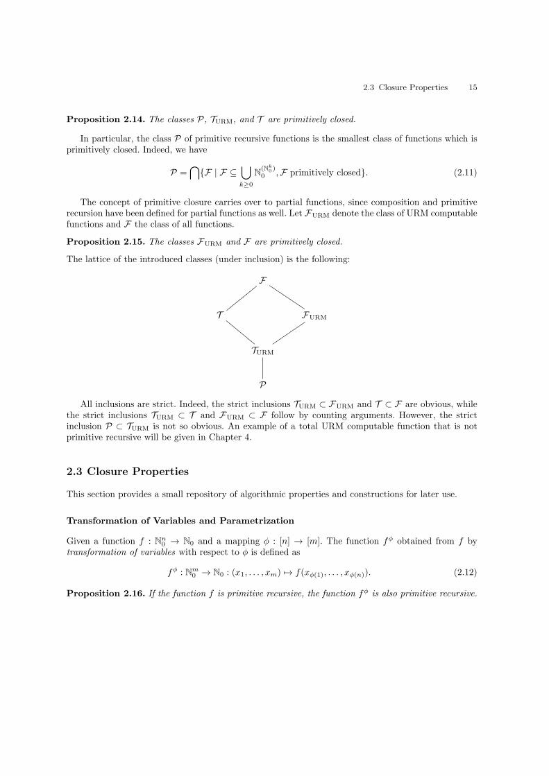
The lattice of the introduced classes (under inclusion) is the following:
F
T
yyyyyyyyyFURM
JJJJJJJJJJ
TURM
uuuuuuuuu
EEEEEEEE
P
All inclusions are strict. Indeed, the strict inclusions TURM ⊂ FURM and T ⊂ F are obvious, whilethe strict inclusions TURM ⊂ T and FURM ⊂ F follow by counting arguments. However, the strictinclusion P ⊂ TURM is not so obvious. An example of a total URM computable function that is notprimitive recursive will be given in Chapter 4.
2.3 Closure Properties
This section provides a small repository of algorithmic properties and constructions for later use.
Transformation of Variables and Parametrization
Given a function f : Nn0 → N0 and a mapping φ : [n] → [m]. The function fφ obtained from f bytransformation of variables with respect to φ is defined as
fφ : Nm0 → N0 : (x1, . . . , xm) 7→ f(xφ(1), . . . , xφ(n)). (2.12)
Proposition 2.16. If the function f is primitive recursive, the function fφ is also primitive recursive.
16 2 Primitive Recursive Functions
Proof. Transformation of variables can be described by the composition
fφ = f(π(m)φ(1), . . . , π
(m)φ(n)). (2.13)
⊓⊔
Examples 2.17. Three important special cases for dyadic functions:
• permutation of variables: fφ : (x, y) 7→ f(y, x),• adjunct of variables: fφ : (x, y) 7→ f(x),• identification of variables: fφ : x 7→ f(x, x).
♦
Let c(k)i denote the k-ary constant function with value i ∈ N0, i.e.,
c(k)i : Nk0 → N0 : (x1, . . . , xk) 7→ i. (2.14)
Proposition 2.18. The constant function c(k)i is primitive recursive.
Proof. If k = 0, c(0)i = νi c
(0)0 . Otherwise, c
(k)i = νi c
(1)0 π
(k)1 . ⊓⊔
Let f : Nn0 → N0 be a function. Take a positive integer m with m < n and a = (a1, . . . , am) ∈ Nm0 .
The function fa obtained from f by parametrization with respect to a is defined as
fa : Nn−m0 → N0 : (x1, . . . , xn−m) 7→ f(x1, . . . , xn−m, a1, . . . , am). (2.15)
Proposition 2.19. If the function f is primitive recursive, the function fa is also primitive recursive.
Proof. Parametrization can be described by the composition
fa = f(π(n−m)1 , . . . , π
(n−m)n−m , c(n−m)
a1 , . . . , c(n−m)am ). (2.16)
⊓⊔
Definition by Cases
Let hi : Nk0 → N0, 1 ≤ i ≤ r, be total functions with the property that for each x ∈ N
k0 there is a unique
index i ∈ [r] such that hi(x) = 0. That is, the sets Hi = x ∈ Nk0 | hi(x) = 0 form a partition of the
whole set Nk0 . Moreover, let gi : Nk0 → N0, 1 ≤ i ≤ r, be arbitrary total functions. Define the function
f : Nk0 → N0 : x 7→
g1(x) if x ∈ H1,...
...gr(x) if x ∈ Hr.
(2.17)
The function f is clearly total and said to be defined by cases.
Proposition 2.20. If the above functions gi and hi, 1 ≤ i ≤ r, are primitive recursive, the function fis also primitive recursive.
2.3 Closure Properties 17
Proof. In case of r = 2, the function f is given in prefix notation as follows:
f = g1 · csg(h1) + g2 · csg(h2). (2.18)
The general case follows by induction on r. ⊓⊔
Example 2.21. Let csg denote the cosign function, i.e., csg(x) = 0 if x > 0 and csg(x) = 1 if x = 0.The mappings h1 : x 7→ x mod 2 and h2 : x 7→ csg(x mod 2) define a partition of the set N0 into the setof even natural numbers and the set of odd natural numbers. These mappings can be used to define afunction defined by cases as follows:
f(x) =
x/2 if x is even,(x+ 1)/2 if x is odd.
(2.19)
♦
Bounded Sum and Product
Let f : Nk+10 → N0 be a total function. The bounded sum of f is the function
Σf : Nk+10 → N0 : (x1, . . . , xk, y) 7→
y∑
i=0
f(x1, . . . , xk, i) (2.20)
and the bounded product of f is the function
Πf : Nk+10 → N0 : (x1, . . . , xk, y) 7→
y∏
i=0
f(x1, . . . , xk, i). (2.21)
Proposition 2.22. If the function f is primitive recursive, the functions Σf and Πf are also primitiverecursive.
Proof. The function Σf is given as
Σf(x, 0) = f(x, 0) and Σf(x, y + 1) = Σf(x, y) + f(x, y + 1). (2.22)
This corresponds to the primitive recursive scheme Σf = pr(g, h), where g(x) = f(x, 0) and h(x, y, z) =+(f(x, ν(y)), z). The function Πf can be similarly defined. ⊓⊔
Example 2.23. Take the function f : N0 → N0 defined by f(x) = 1 if x = 0 and f(x) = x if x > 0.This function is primitive recursive and thus the bounded product, given as Πf(x) = x! for all x ∈ N0,is primitive recursive. ♦
Bounded Minimalization
Let f : Nk+10 → N0 be a total function. The bounded minimalization of f is the function
µf : Nk+10 → N0 : (x, y) 7→ µ(i ≤ y)[f(x, i) = 0], (2.23)

18 2 Primitive Recursive Functions
where for each (x, y) ∈ Nk+10 ,
µ(i ≤ y)[f(x, i) = 0] =
j if j = mini | i ≤ y ∧ f(x, i) = 0 exists,y + 1 otherwise.
(2.24)
That is, the value µf(x, y) provides the smallest index j with 0 ≤ j ≤ y such that f(x, j) = 0. If thereis no such index, the value is y + 1.
Proposition 2.24. If the function f is primitive recursive, the function µf is also primitive recursive.
Proof. By definition,
µf(x, 0) = sgn(f(x, 0)) (2.25)
and
µf(x, y + 1) =
µf(x, y) if µf(x, y) ≤ y or f(x, y + 1) = 0,y + 2 otherwise.
(2.26)
Define the k + 2-ary functions
g1 : (x, y, z) 7→ z,g2 : (x, y, z) 7→ y + 2,h1 : (x, y, z) 7→ (z − y) · sgn(f(x, y + 1)),h2 : (x, y, z) 7→ csg(h1(x, y, z)).
(2.27)
These functions are primitive recursive. Moreover, the functions h1 and h2 provide a partition of N0.Thus the following function defined by cases is also primitive recursive:
g(x, y, z) =
g1(x, y, z) if h1(x, y, z) = 0,g2(x, y, z) if h2(x, y, z) = 0.
(2.28)
We have h1(x, y, µf(x, y)) = 0 if and only if (µf(x, y)) − y) · sgn(f(x, y + 1)) = 0, which is equivalentto µf(x, y)) ≤ y or f(x, y + 1) = 0. In this case, g1(x, y, µf(x, y)) = µf(x, y + 1). The other casecan be similarly evaluated. It follows that the bounded minimalization µf corresponds to the primitiverecursive scheme µf = pr(s, g), where s : Nk0 → N0 is defined as s(x) = sgn(f(x, 0)) and g is given asabove. ⊓⊔
Example 2.25. Consider the integral division function
÷ : N20 → N0 : (x, y) 7→
⌊x/y⌋ if y > 0,x if y = 0,
(2.29)
where the expression ⌊x/y⌋ means that ⌊x/y⌋ = z if y · z ≥ x and z is minimal with this property. Thusthe value z can be provided by bounded minimalization. To this end, define the function f : N3
0 → N0 :(x, y, z) 7→ csg(y · z −x); that is,
f(x, y, z) =
0 if y · z > x,1 otherwise.
(2.30)

2.3 Closure Properties 19
Applying bounded minimalization to f yields the primitive recursive function
µf(x, y, z) =
smallest j ≤ z with y · j > x if j exists,z + 1 otherwise.
(2.31)
Identification of variables provides the primitive recursive function
(µf)′ : (x, y) 7→ µf(x, y, x), (2.32)
which is given as
(µf)′(x, y) =
smallest j ≤ x with y · j > x if y ≥ 1,x+ 1 if y = 0.
(2.33)
It follows that ÷(x, y) = (µf)′(x, y) − 1. Finally, the remainder of x modulo y is given by rem(x, y) =y −x · ÷(x, y) and thus is also primitive recursive. ♦
Pairing Functions
A pairing function uniquely encodes pairs of natural numbers by single natural numbers. A primitiverecursive bijection from N
20 onto N0 is called a pairing function. In set theory, any pairing function
can be used to prove that the rational numbers have the same cardinality as the natural numbers. Forinstance, the Cantor function J2 : N2
0 → N0 is defined as
J2(m,n) =
(m+ n+ 1
2
)
+m. (2.34)
This function will provide a proof that the cartesian product N20 is denumerable. To this end, write
down the elements of N20 in a table as follows:
(0, 0) (0, 1) (0, 2) (0, 3) (0, 4) . . .(1, 0) (1, 1) (1, 2) (1, 3) . . .(2, 0) (2, 1) (2, 2) . . .(3, 0) (3, 1) . . .(4, 0) . . .. . .
(2.35)
Its kth anti-diagonal is given by the sequence
(0, k), (1, k − 1), . . . , (k, 0). (2.36)
Now generate a list of all elements of N20 by writing down the anti-diagonals in a consecutive manner
starting from the 0-th anti-diagonal:
(0, 0), (0, 1), (1, 0), (0, 2), (1, 1), (2, 0), (0, 3), (1, 2), (2, 1), (3, 0), (0, 4), . . . . (2.37)
Note the kth anti-diagonal consists of k + 1 entries. Thus the pair (m,n) lies at position m in them+ nth anti-diagonal and hence occurs in the list at position
20 2 Primitive Recursive Functions
[1 + 2 + . . .+ (m+ n)] +m =
(m+ n+ 1
2
)
+m. (2.38)
That is, J2(m,n) provides the position of the pair (m,n) in the above list. This shows that the functionJ2 is bijective.
Proposition 2.26. The Cantor function J2 is primitive recursive.
Proof. By using the integral division function ÷, one obtains
J2(m,n) = ÷((m,n) · (m+ n+ 1), 2) +m. (2.39)
Thus J2 is primitive recursive. ⊓⊔
The Cantor function J2 can be inverted by taking coordinate functions K2, L2 : N0 → N0 such that
J−12 (n) = (K2(n), L2(n)), n ∈ N0. (2.40)
In order to define them, take n ∈ N0. Find a number s ≥ 0 such that
1
2s(s+ 1) ≤ n <
1
2(s+ 1)(s+ 2) (2.41)
and put
m = n−1
2s(s+ 1). (2.42)
Then
m = n−1
2s(s+ 1) ≤ [
1
2(s+ 1)(s+ 2)− 1]− [
1
2s(s+ 1)] = s. (2.43)
Finally, set
K2(n) = m and L2(n) = s−m. (2.44)
Proposition 2.27. The coordinate functions K2 and L2 are primitive recursive and the pair (K2, L2)is the inverse of J2.
Proof. Let n ∈ N0. The corresponding number s in (2.41) can be determined by bounded minimalizationas follows:
µ(i ≤ n)[n −1
2s(s+ 1) = 0] =
j if j = mini | i ≤ y ∧ n − 1
2s(s+ 1) = 0 exists,n+ 1 otherwise.
(2.45)
The value j always exists and s = j − 1. Then K2(n) = n−÷(s(s+1), 2) and L2(n) = s−K2(n). Thusboth, K2 and L2 are primitive recursive. Finally, by (2.42) and (2.44), J2(K2(n), L2(n)) = J2(m, s −m) = 1
2s(s+ 1) +m = n and so (2.40) follows. ⊓⊔
This assertion implies that the Cantor function J2 is a pairing function.
2.3 Closure Properties 21
Iteration
The powers of a function f : N0 → N0 are inductively defined as
f0 = idN0and fn+1 = f fn, n ≥ 0. (2.46)
The iteration of a function f : N0 → N0 is given by the function
g : N20 → N0 : (x, y) 7→ fy(x). (2.47)
Example 2.28. Consider the function f : N0 → N0 : x 7→ 2x. The iteration of f is the functiong : N2
0 → N0 given by g(x, y) = 2y · x. ♦
Proposition 2.29. If f is a monadic primitive recursive function, the iteration of f is also primitiverecursive.
Proof. The iteration g of f follows the primitive recursive scheme
g(x, 0) = x (2.48)
and
g(x, y + 1) = f(g(x, y)) = f π(3)3 (x, y, g(x, y)), x, y ∈ N0. (2.49)
⊓⊔
Iteration can also be defined for multivariate functions. For this, let f : Nk0 → Nk0 be a function
defined by coordinate functions fi : Nk0 → N0, 1 ≤ i ≤ k, as follows:
f(x) = (f1(x), . . . , fk(x)), x ∈ Nk0 . (2.50)
Write f = (f1, . . . , fk) and define the powers of f inductively as follows:
f0(x) = x and fn+1(x) = (f1(fn(x)), . . . , fk(f
n(x))), x ∈ Nk0 . (2.51)
These definitions immediately give rise to the following result.
Proposition 2.30. If the functions f = (f1, . . . , fk) are primitive recursive, the powers of f are alsoprimitive recursive.
The iteration of f = (f1, . . . , fk) is defined by the functions
gi : Nk+10 → N0 : (x, y) 7→ (π
(k)i f
y)(x), 1 ≤ i ≤ k. (2.52)
Proposition 2.31. If the functions f = (f1, . . . , fk) are primitive recursive, the iteration of f is alsoprimitive recursive.
Proof. The iteration of f = (f1, . . . , fk) follows the primitive recursive scheme
gi(x, 0) = xi (2.53)
and
gi(x, y + 1) = fi(fy(x)) = fi π
(k+2)k+2 (x, y, gi(x, y)), x ∈ N
k0 , y ∈ N0, 1 ≤ i ≤ k. (2.54)
⊓⊔
22 2 Primitive Recursive Functions
2.4 Primitive Recursive Sets
The studies can be extended to relations given as subsets of Nk0 by taking their characteristic function.Let S be a subset of Nk0 . The characteristic function of S is the function χS : Nk0 → N0 defined by
χS(x) =
1 if x ∈ S,0 otherwise.
(2.55)
A subset S of Nk0 is called primitive if its characteristic function χS is primitive recursive.
Examples 2.32. Here are some primitive basic relations:
1. The equality relation R= = (x, y) ∈ N20 | x = y is primitive, since the corresponding characteristic
function χR=(x, y) = csg(|x− y|) is primitive recursive.
2. The inequality relation R 6= = (x, y) ∈ N20 | x 6= y is primitive, since its characteristic function
χR 6=(x, y) = 1− csg(|x− y|) is primitive recursive.
3. The smaller relation R< = (x, y) ∈ N20 | x < y is primitive, since the associated characteristic
function χR<(x, y) = sgn(y −x) is primitive recursive.
♦
Proposition 2.33. If S and T are primitive subsets of Nk0 , S∪T , S∩T , and N
k0 \S are also primitive.
Proof. Clearly, χS∪T (x) = sgn(χS(x) + χT (x)), χS∩T (x) = χS(x) · χT (x), and χNk0\S
(x) = csg χS(x).⊓⊔
Let S be a subset of Nk+10 . The bounded existential quantification of S is a subset of Nk+1
0 given as
∃S = (x, y) | (x, i) ∈ S for some 0 ≤ i ≤ y. (2.56)
The bounded universal quantification of S is a subset of Nk+10 defined by
∀S = (x, y) | (x, i) ∈ S for all 0 ≤ i ≤ y. (2.57)
Proposition 2.34. If S is a primitive subset of Nk+10 , the sets ∃S and ∀S are also primitive.
Proof. Clearly, χ∃S(x, y) = sgn((ΣχS)(x, y)) and χ∀S(x, y) = (ΠχS)(x, y). ⊓⊔
Consider the sequence of increasing primes (p0, p1, p2, p3, p4, . . .) = (2, 3, 5, 7, 11, . . .). By the funda-mental theorem of arithmetics, each natural number x ≥ 1 can be uniquely written as a product ofprime powers, i.e.,
x =
r−1∏
i=0
peii , e0, . . . , er−1 ∈ N0. (2.58)
Write (x)i = ei for each i ∈ N0, and put (0)i = 0 for all i ∈ N0. For instance, 24 = 23 · 3 and so(24)0 = 3, (24)1 = 1, and (24)i = 0 for all i ≥ 2.
Proposition 2.35. 1. The divisibility relation D = (x, y) ∈ N20 | x divides y is primitive.
2.5 LOOP Programs 23
2. The set of primes is primitive.3. The function p : N0 → N0 : i 7→ pi is primitive recursive.4. The function p : N2
0 → N0 : (x, i) 7→ (x)i is primitive recursive.
Proof. First, x divides y, written x | y, if and only if x · i = y for some 0 ≤ i ≤ y. Thus the characteristicfunction of D can be written as
χD(x, y) = sgn[χ=(x · 1, y) + χ=(x · 2, y) + . . .+ χ=(x · y, y)]. (2.59)
Hence the relation D is primitive.Second, a number x is prime if and only if x ≥ 2 and i divides x implies i = 1 or i = x for all
i ≤ x. Thus the characteristic function of the set P of primes is given as follows: χP (0) = χP (1) = 0,χP (2) = 1, and
χP (x) = csg[χD(2, x) + χD(3, x) + . . .+ χD(x− 1, x)], x ≥ 3. (2.60)
Third, define the functions
g(z, x) = |χR<(z, x) · χP (x)− 1| =
0 if z < x and x prime,1 otherwise,
(2.61)
and
h(z) = µg(z, z! + 1) = µ(y ≤ z! + 1)[g(z, y) = 0]. (2.62)
Both functions g and h are primitive recursive. By a theorem of Euclid, the i + 1th prime is boundedby the ith prime in a way that pi+1 ≤ pi!+1 for all i ≥ 0. Thus the value h(pi) provides the next primepi+1. That is, the sequence of prime numbers is given by the primitive recursive scheme
p0 = 2 and pi+1 = h(pi), i ≥ 0. (2.63)
Fourth, we have
(x)i = µ(y ≤ x)[py+1i 6 | x] = µ(y ≤ x)[χD(p
y+1i , x) = 0]. (2.64)
⊓⊔
2.5 LOOP Programs
This section provides a mechanistic description of the class of primitive recursive functions. For this, aclass of URM computable functions is introduced in which the use of loop variables is restricted. Morespecifically, the only loops or iterations allowed will be of the form (M ;Sσ)σ, where the variable σ doesnot appear in the program M . In this way, the program M cannot manipulate the register Rσ and thusit can be guaranteed that the program M will be carried out n times, where n is the content of theregister Rσ at the start of the computation. Loops of this type allow an explicit control over the loopvariable.
Two abbreviations will be used in the following: If P is an URM program and σ ∈ Z, write [P ]σfor the program (P ;Sσ)σ, and denote the URM program (Sσ)σ by Zσ.
The class PLOOP of LOOP programs is inductively defined as follows:
24 2 Primitive Recursive Functions
1. Define the class of LOOP-0 programs PLOOP(0):a) For each σ ∈ Z, Aσ ∈ PLOOP(0) and Zσ ∈ PLOOP(0).b) For each σ, τ ∈ Z with σ 6= τ and σ 6= 0 6= τ , C(σ, τ) = Zτ ;Z0;C(σ; τ) ∈ PLOOP(0).c) If P,Q ∈ PLOOP(0), then P ;Q ∈ PLOOP(0).
2. Suppose the class of LOOP-n programs PLOOP(n) has already been defined. Define the class ofLOOP-n+ 1 programs PLOOP(n+1):a) Each P ∈ PLOOP(n) belongs to PLOOP(n+1).b) If P,Q ∈ PLOOP(n+1), then P ;Q ∈ PLOOP(n+1).c) if P ∈ PLOOP(n) and σ ∈ Z does not appear in P , then [P ]σ ∈ PLOOP(n+1).
Note that for each ω ∈ Ω, w = C(σ, τ)(ω) is given by
ωn =
0 if n = 0,ωσ if n = σ or n = τ ,ωn otherwise.
(2.65)
That is, the content of register Rσ is copied into register Rτ and the register R0 is set to zero.Note that the LOOP-n programs form as sets a proper hierarchy:
PLOOP(0) ⊂ PLOOP(1) ⊂ PLOOP(2) ⊂ . . . . (2.66)
The class of LOOP programs is defined as as the union of LOOP-n programs for all n ∈ N0:
PLOOP =⋃
n≥0
PLOOP(n). (2.67)
In particular, PLOOP(n) is called the class of LOOP programs of depth n, n ∈ N0.
Proposition 2.36. For each LOOP program P , the function ‖P‖ is total.
Proof. For each LOOP-0 program P , it is clear that the function ‖P‖ is total. Let P be a LOOP-nprogram and let σ ∈ Z such that σ does not appear in P . By induction hypothesis, the function‖P‖ is total. Moreover, ‖[P ]σ‖ = ‖P k‖, where k is the content of register Rσ at the beginning of thecomputation. Thus the function ‖[P ]σ‖ is also total. The remaining cases are clear. ⊓⊔
A function f : Nk0 → N0 is called LOOP-n computable if there is a LOOP-n program P such that‖P‖k,1 = f . Let FLOOP(n) denote the class of all LOOP-n computable functions and define the class ofall LOOP computable functions FLOOP as the union of LOOP-n computable functions for all n ≥ 0:
FLOOP =⋃
n≥0
FLOOP(n). (2.68)
Note that if P is a LOOP-n program, n ≥ 1, and P ′ is the normal program corresponding to P , thenP ′ is also a LOOP-n program.
Example 2.37. The program Sσ does not belong to the basic LOOP programs. But it can be describedby a LOOP-1 program. Indeed, put
P − 1= C(1; 3); [C(2; 1);A2]3. (2.69)
2.5 LOOP Programs 25
Then we have for input x = 0,0 1 2 3 4 . . . registers0 0 0 0 0 . . . initially0 0 0 0 0 . . . C(1; 3)0 0 0 0 0 . . . finally
and for input x ≥ 1,0 1 2 3 4 . . . registers0 x 0 0 0 . . . initially0 x 0 x 0 . . . C(1; 3)0 0 0 x 0 . . . C(2; 1)0 0 1 x 0 . . . A20 0 1 x− 1 0 . . . S3. . .0 1 2 x− 2 0 . . .. . .0 x− 1 x 0 0 . . . finally
It follows that ‖P − 1‖1,1 = ‖S1‖1,1. ♦
The LOOP-n computable functions form a hierarchy but at this stage it is not clear whether it is properor not:
TLOOP(0) ⊆ TLOOP(1) ⊆ TLOOP(2) ⊆ . . . . (2.70)
Theorem 2.38. The class of LOOP computable functions equals the class of primitive recursive func-tions.
Proof. First, claim that each primitive recursive function is LOOP computable. Indeed, the basic prim-itive recursive functions are LOOP computable:
1. 0-ary constant function : ‖Z0‖0,1 = c(0)0 ,
2. monadic constant function : ‖Z1‖1,1 = c(1)0 ,
3. successor function: ‖A1‖1,1 = ν,
4. projection function : ‖Z0‖k,1 = π(k)1 and ‖C(σ; 1)‖k,1 = π
(k)σ , σ 6= 1.
Moreover, the class of LOOP computable functions is closed under composition and primitive recursion.This can be shown as in the proof of Theorem 2.10, where subtraction is replaced by the program in 2.37.But the class of primitive recursive functions is the smallest class of functions that is primitively closed.Hence, all primitive recursive functions are LOOP computable. This proves the claim.
Second, claim that each LOOP computable function is primitive recursive. Indeed, for each LOOPprogram P , let n(P ) denote the largest address (or register number) used in P . For integers m ≥ n(P )and 0 ≤ j ≤ m, consider the functions
k(m+1)j (P ) : Nm+1
0 → N0 : (x0, x1, . . . , xm) 7→ (πj |P |)(x0, x1, . . . , xm, , 0, 0, . . .), (2.71)
where for each j ∈ N0,
26 2 Primitive Recursive Functions
πj : Ω → N0 : (ω0, ω1, ω2, . . .) 7→ ωj . (2.72)
The assertion to be shown is a special case of the following assertion: For all LOOP programs P , for
all integers m ≥ n(P ) and 0 ≤ j ≤ m, the function k(m+1)j (P ) is primitive recursive. The proof makes
use of the inductive definition of LOOP programs.First, let P = Aσ, m ≥ σ and 0 ≤ j ≤ m. Then
k(m+1)j (P ) : x 7→
(ν π(m+1)j )(x) if j = σ,
π(m+1)j (x) otherwise.
(2.73)
Clearly, this function is primitive recursive.Second, let P = Zσ, m ≥ σ and 0 ≤ j ≤ m. We have
k(m+1)j (P ) : x 7→
(c(1)0 π
(m+1)j )(x) if j = σ,
π(m+1)j (x) otherwise.
(2.74)
This function is also primitive recursive.Third, let P = C(σ, τ), where σ 6= τ and σ 6= 0 6= τ , m ≥ n(P ) = maxσ, τ and 0 ≤ j ≤ m. Then
k(m+1)j (P ) : x 7→
(c(1)0 π
(m+1)j )(x) if j = 0,
π(m+1)σ (x) if j = τ ,
π(m+1)j (x) otherwise.
(2.75)
This function is clearly primitive recursive.Fourth, let P = Q;R ∈ PLOOP. By induction, assume that the assertion holds for Q and R. Let
m ≥ n(Q;R) = maxn(Q), n(R) and 0 ≤ j ≤ m. Then
k(m+1)j (P )(x) = (πj P )(x, 0, 0, . . .)
= (πj |R| |Q|)(x, 0, 0, . . .)
= k(m+1)j (R)(k
(m+1)0 (Q)(x), . . . , k(m+1)
m (Q)(x)), (2.76)
= k(m+1)j (R)(k
(m+1)0 (Q), . . . , k(m+1)
m (Q))(x).
Thus k(m+1)j (P ) is a composition of primitive recursive functions and hence also primitive recursive.
Finally, let P = [Q]σ ∈ PLOOP, where Q is a LOOP program in which the address σ is not involved.By induction, assume that the assertion holds for Q. Let m ≥ n([Q]σ) = maxn(Q), σ and 0 ≤ j ≤ m.
First the program Q;Sσ yields
k(m+1)j (Q;Sσ) : x 7→
k(m+1)j (Q)(x) if j 6= σ,
(f − 1 π
(m+1)j )(x) otherwise.
(2.77)
Let k(m+1)(Q;Sσ) : Nm+10 → N
m+10 denote the product of the m + 1 functions k
(m+1)j (Q;Sσ) for
0 ≤ j ≤ m. That is,
k(m+1)(Q;Sσ)(x) = (k(m+1)0 (Q;Sσ)(x), . . . , k(m+1)
m (Q;Sσ)(x)). (2.78)
2.5 LOOP Programs 27
Let g : Nm+20 → N
m+10 denote the iteration of k(m+1)(Q;Sσ); that is,
g(x, 0) = x and g(x, y + 1) = k(m+1)(Q;Sσ)(g(x, y)). (2.79)
For each index j, 0 ≤ j ≤ m, the composition π(m+1)j g is also primitive recursive giving
(π(m+1)j g)(x, y) = k
(m+1)j ((Q;Sσ)y)(x). (2.80)
But the register Rσ is never used by the program Q and thus
|P |(ω) = |(Q;Sσ)σ|(ω) = |(Q;Sσ)ωσ |(ω), ω ∈ Ω. (2.81)
It follows that the function k(m+1)j (P ) can be obtained from the primitive recursive function π
(m+1)j g
by transformation of variables, i.e.,
k(m+1)j (P )(x) = (π
(m+1)j g)(x, π(m+1)
σ (x)), x ∈ Nm+10 . (2.82)
Thus k(m+1)j (P ) is also primitive recursive. ⊓⊔
28 2 Primitive Recursive Functions
3
Partial Recursive Functions
The partial recursive functions form a class of partial functions that are computable in an intuitivesense. In fact, the partial recursive functions are precisely the functions that can be computed by Turingmachines or unlimited register machines. By Church’s thesis, the partial recursive functions provide aformalization of the notion of computability. The partial recursive functions are closely related to theprimitive recursive functions and their inductive definition builds upon them.
3.1 Partial Recursive Functions
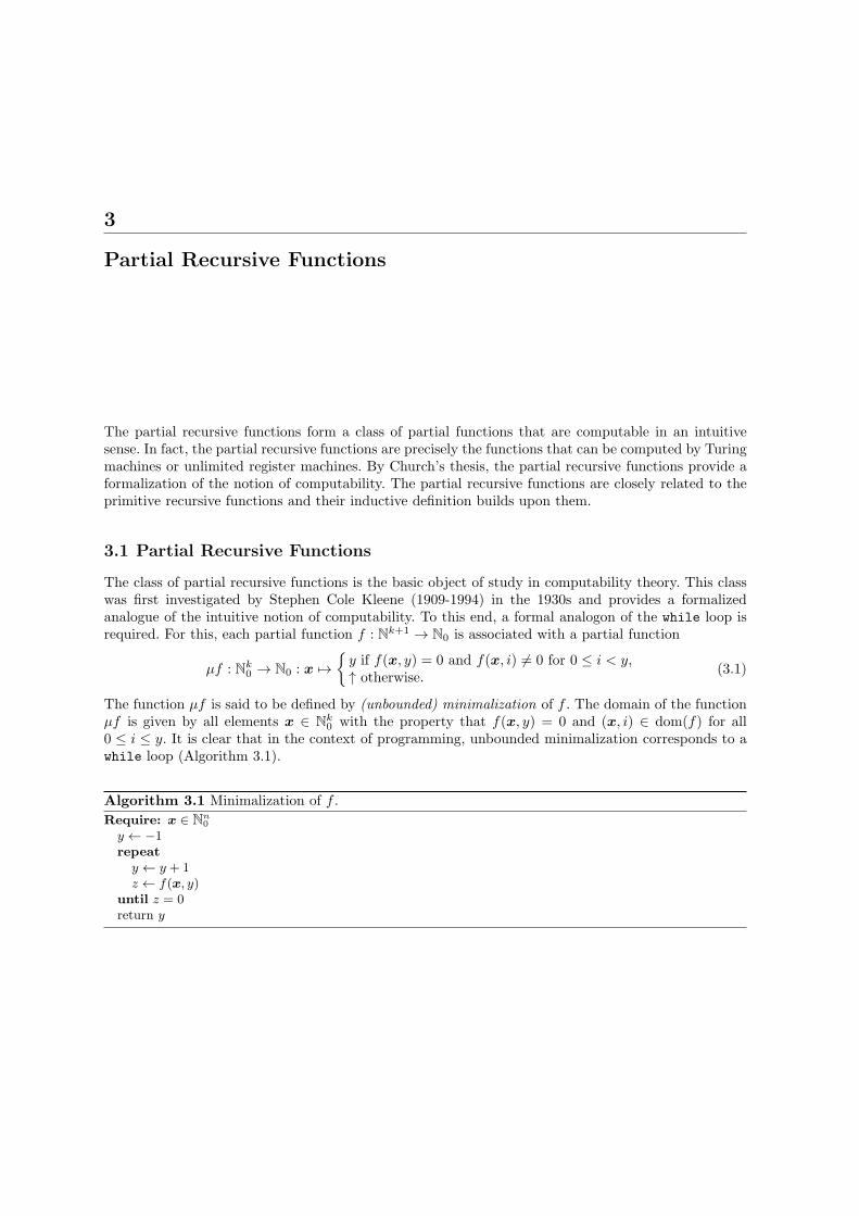
The class of partial recursive functions is the basic object of study in computability theory. This classwas first investigated by Stephen Cole Kleene (1909-1994) in the 1930s and provides a formalizedanalogue of the intuitive notion of computability. To this end, a formal analogon of the while loop isrequired. For this, each partial function f : Nk+1 → N0 is associated with a partial function
µf : Nk0 → N0 : x 7→
y if f(x, y) = 0 and f(x, i) 6= 0 for 0 ≤ i < y,↑ otherwise.
(3.1)
The function µf is said to be defined by (unbounded) minimalization of f . The domain of the functionµf is given by all elements x ∈ N
k0 with the property that f(x, y) = 0 and (x, i) ∈ dom(f) for all
0 ≤ i ≤ y. It is clear that in the context of programming, unbounded minimalization corresponds to awhile loop (Algorithm 3.1).
Algorithm 3.1 Minimalization of f .
Require: x ∈ Nn0
y ← −1repeat
y ← y + 1z ← f(x, y)
until z = 0return y
30 3 Partial Recursive Functions
Examples 3.1.
• The minimalization function µf may be partial even if f is total: The function f(x, y) = (x+ y) − 3is total, while its minimalization µf is partial with dom(µf) = 0, 1, 2, 3 and µf(0) = µf(1) =µf(2) = µf(3) = 0.
• The minimalization function µf may be total even if f is partial: Take the partial function f(x, y) =x − y if y ≤ x and f(x, y) =↑ if y > x. The corresponding minimalization µf(x) = x is total withdom(µf) = N0. ♦
The class R of partial recursive functions over N0 is inductively defined:
• R contains all the base functions.• If partial functions g : Nk0 → N0 and hi : N
n0 → N0, 1 ≤ i ≤ k, belong to R, the composite function
f = g(h1, . . . , hk) : Nn0 → N0 is in R.
• If partial functions g : Nn0 → N0 and h : Nn+20 → N0 lie in R, the primitive recursion f = pr(g, h) :
Nn+10 → N0 is contained in R.
• If a partial function f : Nn+10 → N0 is in R, the partial function µf : N
n0 → N0 obtained by
minimalization belongs to R.
Thus the class R consists of all partial recursive functions obtained from the base functions by finitelymany applications of composition, primitive recursion, and minimalization. In particular, each totalpartial recursive function is called a recursive function, and the subclass of all total partial recursivefunctions is denoted by T . It is clear that the class P of primitive recursive functions is a subclass ofthe class T of recursive functions.
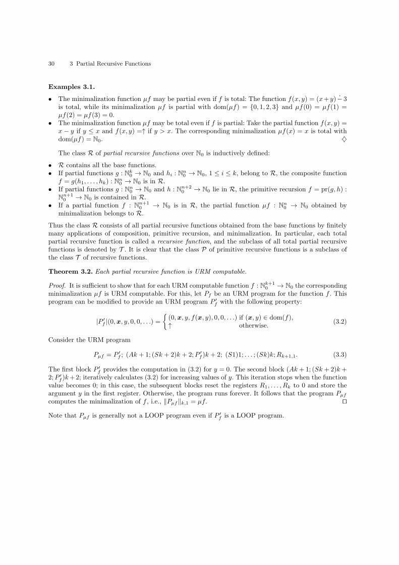
Theorem 3.2. Each partial recursive function is URM computable.
Proof. It is sufficient to show that for each URM computable function f : Nk+10 → N0 the corresponding
minimalization µf is URM computable. For this, let Pf be an URM program for the function f . Thisprogram can be modified to provide an URM program P ′
f with the following property:
|P ′f |(0,x, y, 0, 0, . . .) =
(0,x, y, f(x, y), 0, 0, . . .) if (x, y) ∈ dom(f),↑ otherwise.
(3.2)
Consider the URM program
Pµf = P ′f ; (Ak + 1; (Sk + 2)k + 2;P ′
f )k + 2; (S1)1; . . . ; (Sk)k;Rk+1,1. (3.3)
The first block P ′f provides the computation in (3.2) for y = 0. The second block (Ak + 1; (Sk + 2)k +
2;P ′f )k+2; iteratively calculates (3.2) for increasing values of y. This iteration stops when the function
value becomes 0; in this case, the subsequent blocks reset the registers R1, . . . , Rk to 0 and store theargument y in the first register. Otherwise, the program runs forever. It follows that the program Pµfcomputes the minimalization of f , i.e., ‖Pµf‖k,1 = µf. ⊓⊔
Note that Pµf is generally not a LOOP program even if P ′f is a LOOP program.
3.2 GOTO Programs 31
3.2 GOTO Programs
GOTO programs offer another way to formalize the notion of computability. They are closely relatedto programs in BASIC or FORTRAN.
First, define the syntax of GOTO programs. For this, let V = xn | n ∈ N be a set of variables.The instructions of a GOTO program are the following:
• incrementation:
(l, xσ ← xσ + 1,m), l,m ∈ N0, xσ ∈ V, (3.4)
• decrementation:
(l, xσ ← xσ − 1,m), l,m ∈ N0, xσ ∈ V, (3.5)
• conditionals:
(l, if xσ = 0, k,m), k, l,m ∈ N0, xσ ∈ V. (3.6)
The first component of an instruction, denoted by l, is called a label, the third component of aninstruction (l, xσ+,m) or (l, xσ−,m), denoted by m, is termed next label, and the last two componentsof an instruction (l, if xσ = 0, k,m), denoted by k and m, are called bifurcation labels.
A GOTO program is given by a finite sequence of GOTO instructions
P = s0; s1; . . . ; sq, (3.7)
such that there is a unique instruction si which has the label λ(si) = 0, 0 ≤ i ≤ q, and differentinstructions have distinct labels, i.e., for 0 ≤ i < j ≤ q, λ(si) 6= λ(sj).
In the following, let PGOTO denote the class of all GOTO programs. Moreover, for each GOTOprogram P , let V (P ) depict the set of variables occurring in P and L(P ) = λ(si) | 0 ≤ i ≤ q describethe set of labels in P .
A GOTO program P = s0; s1; . . . ; sq is called standard if the ith instruction si carries the labelλ(si) = i, 0 ≤ i ≤ q.
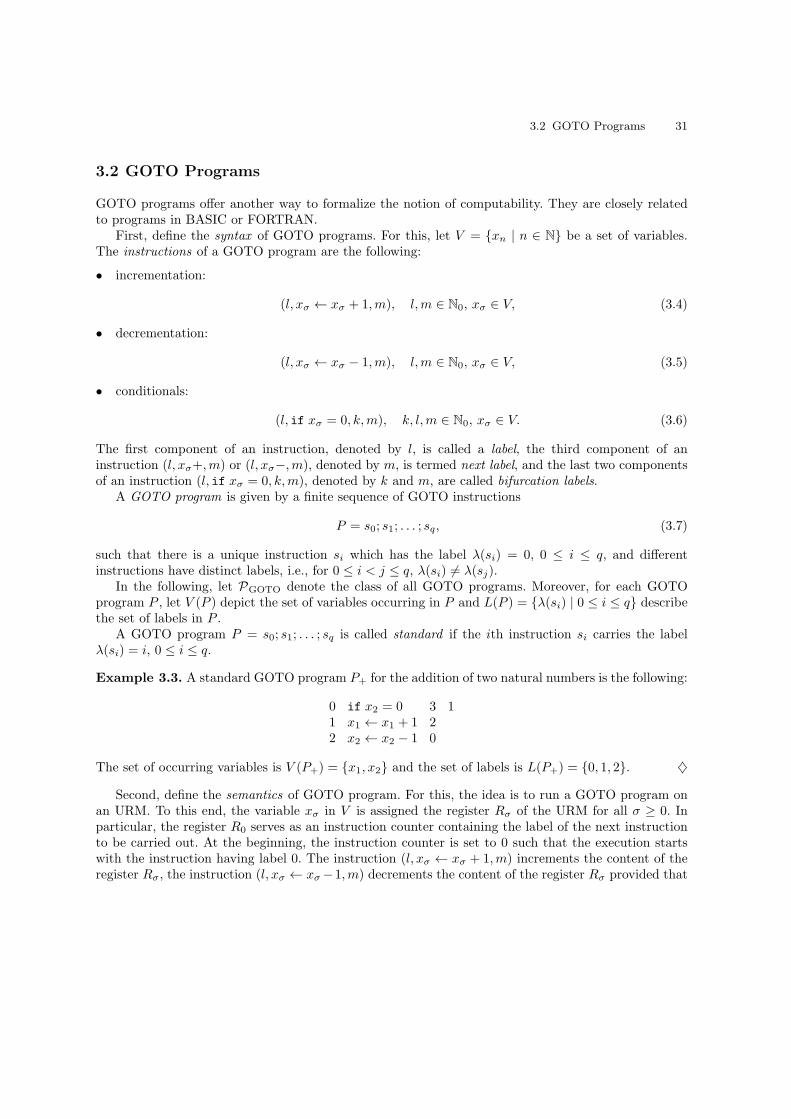
Example 3.3. A standard GOTO program P+ for the addition of two natural numbers is the following:
0 if x2 = 0 3 11 x1 ← x1 + 1 22 x2 ← x2 − 1 0
The set of occurring variables is V (P+) = x1, x2 and the set of labels is L(P+) = 0, 1, 2. ♦
Second, define the semantics of GOTO program. For this, the idea is to run a GOTO program onan URM. To this end, the variable xσ in V is assigned the register Rσ of the URM for all σ ≥ 0. Inparticular, the register R0 serves as an instruction counter containing the label of the next instructionto be carried out. At the beginning, the instruction counter is set to 0 such that the execution startswith the instruction having label 0. The instruction (l, xσ ← xσ + 1,m) increments the content of theregister Rσ, the instruction (l, xσ ← xσ−1,m) decrements the content of the register Rσ provided that

32 3 Partial Recursive Functions
it contains a number greater than zero, and the conditional statement (l, if xσ = 0, k,m) provides ajump to the statement with label k if the content of register Rσ is 0; otherwise, a jump is performed tothe statement with labelm. The execution of a GOTO program terminates if the label of the instructioncounter does not correspond to an instruction.
More specifically, let P be a GOTO program and k be a number. Define the partial function
‖P‖k,1 = β1 RP αk, (3.8)
where αk and β1 are total functions given by
αk : Nk0 → Nn+10 : (x1, x2, . . . , xk) 7→ (0, x1, x2, . . . , xk, 0, 0, . . . , 0) (3.9)
and
β1 : Nn+10 → N0 : (x0, x1, . . . , xn) 7→ x1. (3.10)
The function αk loads the registers with the arguments and the function β1 reads out the result. Notethat the number n needs to be chosen large enough to provide sufficient workspace for the computation;that is,
n ≥ maxk,maxσ | xσ ∈ V (P ). (3.11)
Finally, the function RP : Nn+10 → N
n+10 providing the semantics of the program P will be formally
described. For this, let P = s0; s1; . . . ; sq be a GOTO program. Each element z = (z0, z1, . . . , zn) inNn+10 is called a configuration. We say that the configuration z′ = (z′0, z
′1, . . . , z
′n) is reached in one step
from the configuration z = (z0, z1, . . . , zn), written z ⊢P z′, if z0 is a label in P , say z0 = λ(si) forsome 0 ≤ i ≤ q, and
• if si = (z0, xσ ← xσ + 1,m),
z′ = (m, z1, . . . , zσ−1, zσ + 1, zσ+1, . . . , zn), (3.12)
• if si = (z0, xσ ← xσ − 1,m),
z′ = (m, z1, . . . , zσ−1, zσ − 1, zσ+1, . . . , zn), (3.13)
• if si = (z0, if xσ = 0, k,m),
z′ =
(k, z1, . . . , zn) if zσ = 0,(m, z1, . . . , zn) otherwise.
(3.14)
The configuration z′ is called the successor configuration of z. Moreover, if z0 is not a label in P , thereis no successor configuration of z and the successor configuration is undefined. The process to movefrom one configuration to the next one can be described by the one-step function EP : Nn+1
0 → Nn+10
defined as
EP : z 7→
z′ if z ⊢P z′,z otherwise.
(3.15)
The function EP is given by cases and has the following property.
3.2 GOTO Programs 33
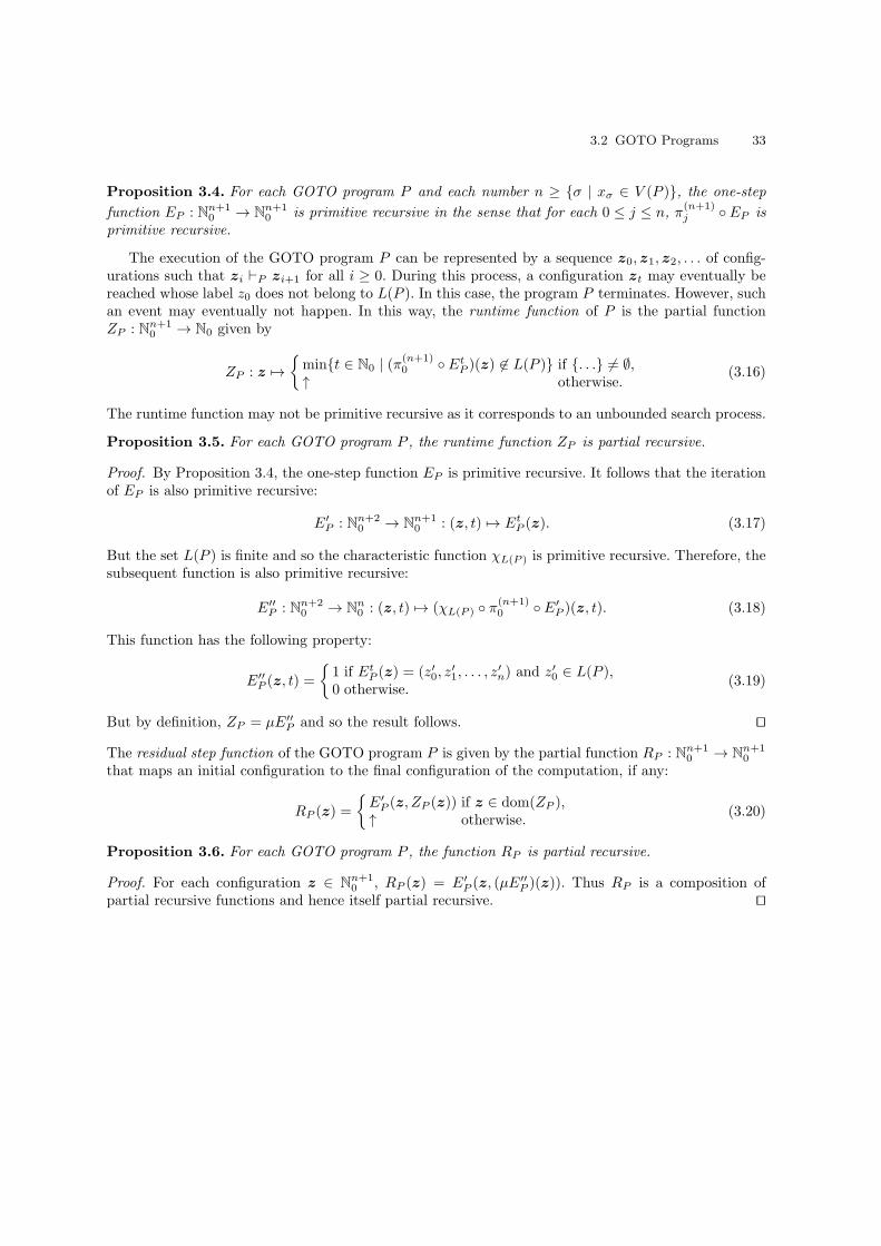
Proposition 3.4. For each GOTO program P and each number n ≥ σ | xσ ∈ V (P ), the one-step
function EP : Nn+10 → N
n+10 is primitive recursive in the sense that for each 0 ≤ j ≤ n, π
(n+1)j EP is
primitive recursive.
The execution of the GOTO program P can be represented by a sequence z0, z1, z2, . . . of config-urations such that zi ⊢P zi+1 for all i ≥ 0. During this process, a configuration zt may eventually bereached whose label z0 does not belong to L(P ). In this case, the program P terminates. However, suchan event may eventually not happen. In this way, the runtime function of P is the partial functionZP : Nn+1
0 → N0 given by
ZP : z 7→
mint ∈ N0 | (π(n+1)0 EtP )(z) 6∈ L(P ) if . . . 6= ∅,
↑ otherwise.(3.16)
The runtime function may not be primitive recursive as it corresponds to an unbounded search process.
Proposition 3.5. For each GOTO program P , the runtime function ZP is partial recursive.
Proof. By Proposition 3.4, the one-step function EP is primitive recursive. It follows that the iterationof EP is also primitive recursive:
E′P : Nn+2
0 → Nn+10 : (z, t) 7→ EtP (z). (3.17)
But the set L(P ) is finite and so the characteristic function χL(P ) is primitive recursive. Therefore, thesubsequent function is also primitive recursive:
E′′P : Nn+2
0 → Nn0 : (z, t) 7→ (χL(P ) π
(n+1)0 E′
P )(z, t). (3.18)
This function has the following property:
E′′P (z, t) =
1 if EtP (z) = (z′0, z
′1, . . . , z
′n) and z
′0 ∈ L(P ),
0 otherwise.(3.19)
But by definition, ZP = µE′′P and so the result follows. ⊓⊔
The residual step function of the GOTO program P is given by the partial function RP : Nn+10 → N
n+10
that maps an initial configuration to the final configuration of the computation, if any:
RP (z) =
E′P (z, ZP (z)) if z ∈ dom(ZP ),↑ otherwise.
(3.20)
Proposition 3.6. For each GOTO program P , the function RP is partial recursive.
Proof. For each configuration z ∈ Nn+10 , RP (z) = E′
P (z, (µE′′P )(z)). Thus RP is a composition of
partial recursive functions and hence itself partial recursive. ⊓⊔
34 3 Partial Recursive Functions
3.3 GOTO Computable Functions
A partial function f : Nk0 → N0 is called GOTO computable if there is a GOTO program P that
computes f in the sense that
f = ‖P‖k,1. (3.21)
Let FGOTO denote the class of all (partial) GOTO computable functions and let TGOTO depict theclass of all total GOTO computable functions.
Theorem 3.7. Each GOTO computable function is partial recursive, and each total GOTO computablefunction is recursive.
Proof. If f is GOTO computable, there is a GOTO program such that f = ‖P‖k,1 = β1 RP αk.But the functions β1 and αk are primitive recursive and the function RP is partial recursive. Thus thecomposition is partial recursive. In particular, if f is total, then RP is also total and so f is recursive.⊓⊔
Example 3.8. The GOTO program P+ for the addition of two natural numbers in Example 3.3 givesrise to the following configurations if x2 > 0:
(0, x1, x2) 0 if x2 = 0 3 1(1, x1, x2) 1 x1 ← x1 + 1 2(2, x1 + 1, x2) 2 x2 ← x2 − 1 0(0, x1 + 1, x2 − 1) 3 if x2 = 0 3 1. . .
Clearly, this program provides the addition function ‖P+‖2,1(x1, x2) = x1 + x2. ♦
Finally, it will be shown that URM programs can be translated into GOTO programs.
Theorem 3.9. Each URM computable function is GOTO computable.
Proof. Claim that each URM program P can be compiled into a GOTO program φ(P ) such that bothcompute the same function, i.e., ‖P‖k,1 = ‖φ(P )‖k,1 for all k ∈ N. Indeed, let P be an URM program.We may assume that it does not make use of the register R0. Write P as a string P = τ0τ1 . . . τq, whereeach substring τi is of the form ”Aσ”, ”Sσ”, ”(” or ”)σ” with σ ∈ Z \ 0. Note that each openingparenthesis ”(” corresponds to a unique closing parenthesis ”)σ”.
Replace each string τi by a GOTO instruction si as follows:
• If τi = ”Aσ”, putsi = (i, xσ ← xσ + 1, i+ 1),
• if τi = ”Sσ”, setsi = (i, xσ ← xσ − 1, i+ 1),
• if τi = ”(” and τj = ”)σ” is the corresponding closing parenthesis, define
si = (i, if xσ = 0, j + 1, i+ 1),

3.4 GOTO-2 Programs 35
• if τi = ”)σ” and τj = ”(” is the associated opening parenthesis, put
si = (i, if xσ = 0, i+ 1, j + 1).
In this way, a GOTO program φ(P ) = s0; s1; . . . ; sq is established that has the required property‖P‖k,1 = ‖φ(P )‖k,1, as claimed. ⊓⊔
Example 3.10. The URM program P = (A1;S2)2 provides the addition of two natural numbers. Itstranslation into a GOTO program first requires to identify the substrings:
τ0 = ”(”, τ1 = ”A1”, τ2 = ”S2”, τ3 = ”)2”.
These substrings give rise to the following GOTO program:
0 if x2 = 0 4 11 x1 ← x1 + 1 22 x2 ← x2 − 1 33 if x2 = 0 4 1
♦
3.4 GOTO-2 Programs
GOTO-2 programs are GOTO programs with two variables x1 and x2. Claim that each URM programcan be simulated by an appropriate GOTO-2 program. For this, the set of states Ω of an URM isencoded by using the sequence of primes (p0, p1, p2, . . .). To this end, define the function G : Ω → N0
that assigns to each state ω = (ω0, ω1, ω2, . . .) ∈ Ω the natural number
G(ω) = pω00 pω1
1 pω22 . . . . (3.22)
Clearly, this function is primitive recursive. The inverse functions Gi : N0 → N0, i ∈ N0, are given by
Gi(x) = (x)i, (3.23)
where (x)i is the exponent of pi in the prime factorization of x if x > 0. Define Gi(0) = 0 for all i ∈ N0.The functions Gi are primitive recursive by Proposition 2.35.
Claim that for each URM program P , there is a GOTO-2 program P with the same semantics; thatis, for all states ω, ω′ ∈ Ω,
|P |(ω) = ω′ ⇐⇒ |P |(0, G(ω)) = (0, G(ω′)). (3.24)
To see this, first consider the GOTO-2 programsM(k), D(k), and T (k), k ∈ N, which have the followingproperties:
|M(k)|(0, x) = (0, k · x), (3.25)
|D(k)|(0, k · x) = (0, x), (3.26)
|T (k)|(0, x) =
(1, x) if k divides x,(0, x) otherwise.
(3.27)
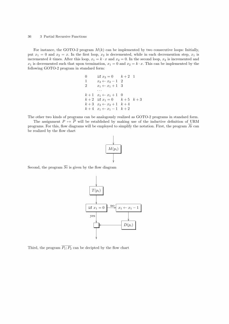
36 3 Partial Recursive Functions
For instance, the GOTO-2 program M(k) can be implemented by two consecutive loops: Initially,put x1 = 0 and x2 = x. In the first loop, x2 is decremented, while in each decremention step, x1 isincremented k times. After this loop, x1 = k · x and x2 = 0. In the second loop, x2 is incremented andx1 is decremented such that upon termination, x1 = 0 and x2 = k · x. This can be implemented by thefollowing GOTO-2 program in standard form:
0 if x2 = 0 k + 2 11 x2 ← x2 − 1 22 x1 ← x1 + 1 3
· · ·k + 1 x1 ← x1 + 1 0k + 2 if x1 = 0 k + 5 k + 3k + 3 x2 ← x2 + 1 k + 4k + 4 x1 ← x1 − 1 k + 2
The other two kinds of programs can be analogously realized as GOTO-2 programs in standard form.The assignment P 7→ P will be established by making use of the inductive definition of URM
programs. For this, flow diagrams will be employed to simplify the notation. First, the program Ai canbe realized by the flow chart
M(pi)
Second, the program Si is given by the flow diagram
T (pi)
if x1 = 0
no //
yes
x1 ← x1 − 1
D(pi)oo
Third, the program P1;P2 can be decipted by the flow chart
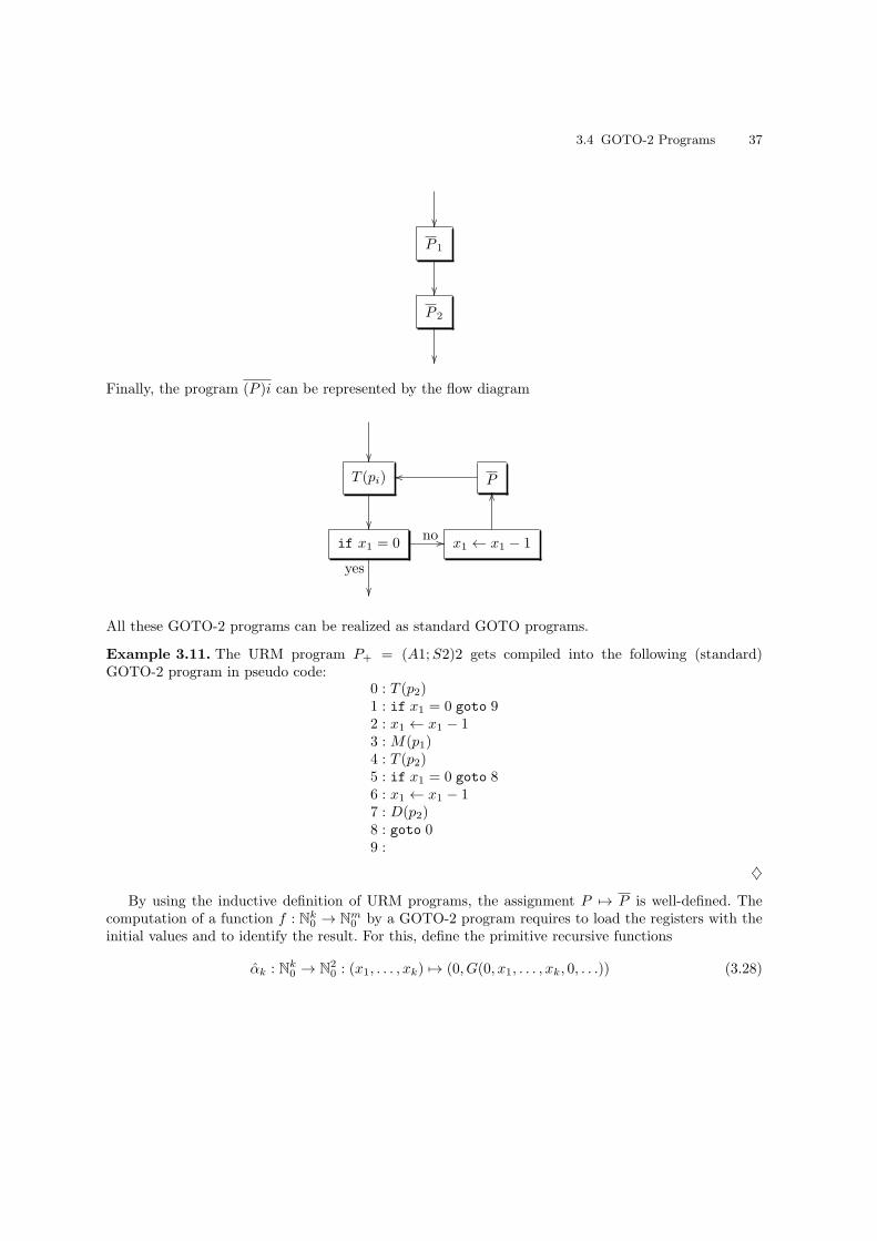
3.4 GOTO-2 Programs 37
P 1
P 2
Finally, the program (P )i can be represented by the flow diagram
T (pi)
Poo
if x1 = 0no //
yes
x1 ← x1 − 1
OO
All these GOTO-2 programs can be realized as standard GOTO programs.
Example 3.11. The URM program P+ = (A1;S2)2 gets compiled into the following (standard)GOTO-2 program in pseudo code:
0 : T (p2)1 : if x1 = 0 goto 92 : x1 ← x1 − 13 : M(p1)4 : T (p2)5 : if x1 = 0 goto 86 : x1 ← x1 − 17 : D(p2)8 : goto 09 :
♦
By using the inductive definition of URM programs, the assignment P 7→ P is well-defined. Thecomputation of a function f : Nk0 → N
m0 by a GOTO-2 program requires to load the registers with the
initial values and to identify the result. For this, define the primitive recursive functions
αk : Nk0 → N20 : (x1, . . . , xk) 7→ (0, G(0, x1, . . . , xk, 0, . . .)) (3.28)
38 3 Partial Recursive Functions
and
βm : N20 → N
m0 : (a, b) 7→ (G1(b), . . . , Gm(b)). (3.29)
Proposition 3.12. Each URM program P is (semantically) equivalent to the associated GOTO-2 pro-gram P in the sense that for all k,m ∈ N0:
‖P‖k,m = βm RP αk. (3.30)
3.5 Church’s Thesis
Our attempts made so far to formalize the notion of computability are equivalent in the following sense.
Theorem 3.13. The class of partial recursive functions equals the class of URM computable functionsand the class of GOTO computable functions. In particular, the class of recursive functions is equal tothe class of total URM computable functions and to the class of total GOTO computable functions.
Proof. By Theorem 3.9, each URM computable function is GOTO computable and by Theorem 3.7,each GOTO computable function is partial recursive. On the other hand, by Theorem 3.2, each partialrecursive function is URM computable. A similar statement holds for total functions. ⊓⊔
This result has led scientists to believe that the concept of computability is accurately characterizedby the class of partial recursive functions. The Church thesis proposed by Alonso Church (1903-1995)in the 1930s states that the class of computable partial functions (in the intuitive sense) coincides withthe class of partial recursive functions, equivalently, with the class of URM computable functions andthe class of GOTO computable functions. Church’s thesis characterizes the nature of computation andcannot be formally proved. Nevertheless, today, it has universal acceptance. Church’s thesis is oftenpractically used in the sense that if a (partial) function is intuitively computable, it is assumed tobe partial recursive. In this way, the thesis may lead to more intuitive and less rigorous proofs (seeTheorem 5.10).
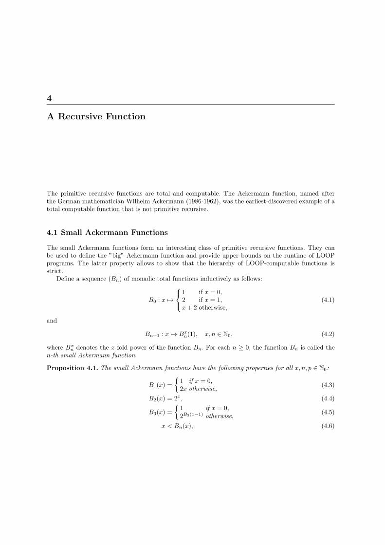
4
A Recursive Function
The primitive recursive functions are total and computable. The Ackermann function, named afterthe German mathematician Wilhelm Ackermann (1986-1962), was the earliest-discovered example of atotal computable function that is not primitive recursive.
4.1 Small Ackermann Functions
The small Ackermann functions form an interesting class of primitive recursive functions. They canbe used to define the ”big” Ackermann function and provide upper bounds on the runtime of LOOPprograms. The latter property allows to show that the hierarchy of LOOP-computable functions isstrict.
Define a sequence (Bn) of monadic total functions inductively as follows:
B0 : x 7→
1 if x = 0,2 if x = 1,x+ 2 otherwise,
(4.1)
and
Bn+1 : x 7→ Bxn(1), x, n ∈ N0, (4.2)
where Bxn denotes the x-fold power of the function Bn. For each n ≥ 0, the function Bn is called then-th small Ackermann function.
Proposition 4.1. The small Ackermann functions have the following properties for all x, n, p ∈ N0:
B1(x) =
1 if x = 0,2x otherwise,
(4.3)
B2(x) = 2x, (4.4)
B3(x) =
1 if x = 0,2B3(x−1) otherwise,
(4.5)
x < Bn(x), (4.6)

40 4 A Recursive Function
Bn(x) < Bn(x+ 1), (4.7)
Bp0(x) ≤ Bp1(x), (4.8)
Bn(x) ≤ Bn+1(x), (4.9)
Bpn(x) < Bpn(x+ 1), (4.10)
Bpn(x) < Bp+1n (x), (4.11)
Bpn(x) ≤ Bpn+1(x), (4.12)
2p+1x ≤ Bp+11 (x), (4.13)
2Bpn(x) ≤ Bp+1n (x), n ≥ 1. (4.14)
Proposition 4.2. The small Ackermann functions Bn, n ∈ N0, are primitive recursive.
Proof. The function B0 is defined by cases:
B0(x) =
(ν c(1)0 )(x) if x = 0,
(ν ν c(1)0 )(x) if |x − 1| = 0,
(ν ν π(1)1 )(x) otherwise.
(4.15)
By Eq. (4.3), the function B1 follows the primitive recursive scheme
B1(0) = 1, (4.16)
B1(x+ 1) = B1(x) · sgn(x) + 2, x ∈ N0. (4.17)
Finally, if n ≥ 2, Bn is given by the primitive recursive scheme
Bn(0) = 1, (4.18)
Bn(x+ 1) = Bn−1(Bn(x)), x ∈ N0. (4.19)
By induction, the small Ackermann functions are primitive recursive. ⊓⊔
The n+ 1th small Ackermann function grows faster than any power of the nth Ackermann function inthe following sense.
Proposition 4.3. For all number n and p, there is a number x0 such that for all numbers x ≥ x0,
Bpn(x) < Bn+1(x). (4.20)
Proof. Let n = 0. For each x ≥ 2, Bp0(x) = x+2p. On the other hand, for each x ≥ 1, B1(x) = 2x. Putx0 = 2p+ 1. Then for each x ≥ x0,
Bp0(x) = x+ 2p ≤ 2x = B1(x).
Let n > 0. First, let p = 0. Then for each x ≥ 0,
B0n(x) = x < Bn(x) ≤ Bn+1(x)
by (4.6) and (4.9). Second, let p > 0 and assume that Bpn(x) < Bn+1(x) holds for all x ≥ x′0. Putx0 = x′0 + 5. Then
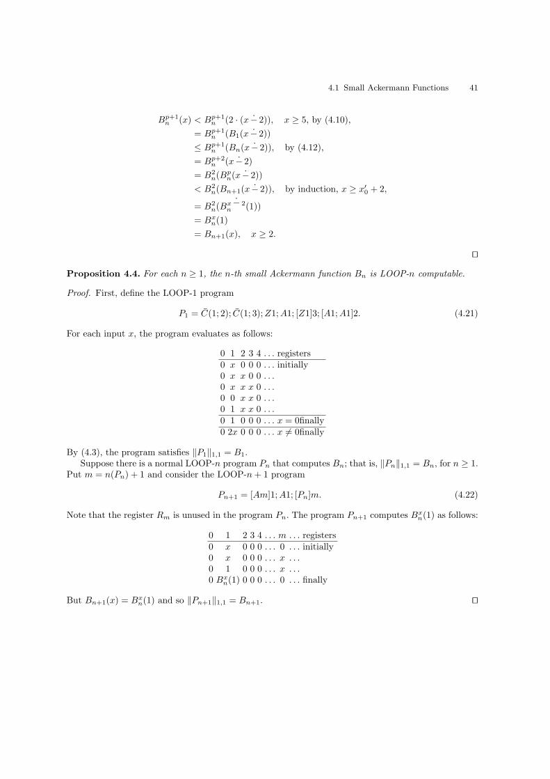
4.1 Small Ackermann Functions 41
Bp+1n (x) < Bp+1
n (2 · (x − 2)), x ≥ 5, by (4.10),
= Bp+1n (B1(x − 2))
≤ Bp+1n (Bn(x − 2)), by (4.12),
= Bp+2n (x − 2)
= B2n(B
pn(x − 2))
< B2n(Bn+1(x − 2)), by induction, x ≥ x′0 + 2,
= B2n(B
x − 2n (1))
= Bxn(1)
= Bn+1(x), x ≥ 2.
⊓⊔
Proposition 4.4. For each n ≥ 1, the n-th small Ackermann function Bn is LOOP-n computable.
Proof. First, define the LOOP-1 program
P1 = C(1; 2); C(1; 3);Z1;A1; [Z1]3; [A1;A1]2. (4.21)
For each input x, the program evaluates as follows:
0 1 2 3 4 . . . registers0 x 0 0 0 . . . initially0 x x 0 0 . . .0 x x x 0 . . .0 0 x x 0 . . .0 1 x x 0 . . .0 1 0 0 0 . . . x = 0finally0 2x 0 0 0 . . . x 6= 0finally
By (4.3), the program satisfies ‖P1‖1,1 = B1.Suppose there is a normal LOOP-n program Pn that computes Bn; that is, ‖Pn‖1,1 = Bn, for n ≥ 1.
Put m = n(Pn) + 1 and consider the LOOP-n+ 1 program
Pn+1 = [Am]1;A1; [Pn]m. (4.22)
Note that the register Rm is unused in the program Pn. The program Pn+1 computes Bxn(1) as follows:
0 1 2 3 4 . . . m . . . registers0 x 0 0 0 . . . 0 . . . initially0 x 0 0 0 . . . x . . .0 1 0 0 0 . . . x . . .0 Bxn(1) 0 0 0 . . . 0 . . . finally
But Bn+1(x) = Bxn(1) and so ‖Pn+1‖1,1 = Bn+1. ⊓⊔
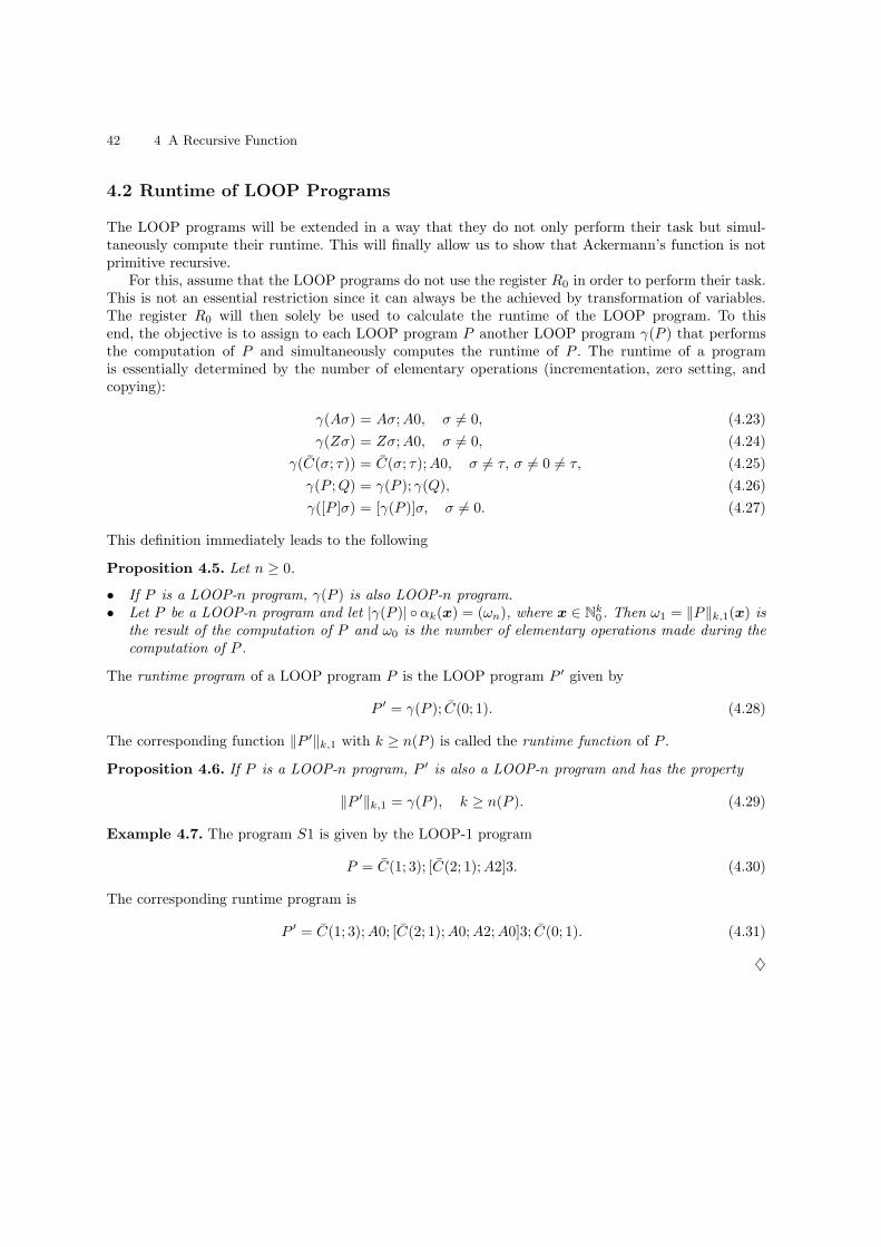
42 4 A Recursive Function
4.2 Runtime of LOOP Programs
The LOOP programs will be extended in a way that they do not only perform their task but simul-taneously compute their runtime. This will finally allow us to show that Ackermann’s function is notprimitive recursive.
For this, assume that the LOOP programs do not use the register R0 in order to perform their task.This is not an essential restriction since it can always be the achieved by transformation of variables.The register R0 will then solely be used to calculate the runtime of the LOOP program. To thisend, the objective is to assign to each LOOP program P another LOOP program γ(P ) that performsthe computation of P and simultaneously computes the runtime of P . The runtime of a programis essentially determined by the number of elementary operations (incrementation, zero setting, andcopying):
γ(Aσ) = Aσ;A0, σ 6= 0, (4.23)
γ(Zσ) = Zσ;A0, σ 6= 0, (4.24)
γ(C(σ; τ)) = C(σ; τ);A0, σ 6= τ, σ 6= 0 6= τ, (4.25)
γ(P ;Q) = γ(P ); γ(Q), (4.26)
γ([P ]σ) = [γ(P )]σ, σ 6= 0. (4.27)
This definition immediately leads to the following
Proposition 4.5. Let n ≥ 0.
• If P is a LOOP-n program, γ(P ) is also LOOP-n program.• Let P be a LOOP-n program and let |γ(P )| αk(x) = (ωn), where x ∈ N
k0 . Then ω1 = ‖P‖k,1(x) is
the result of the computation of P and ω0 is the number of elementary operations made during thecomputation of P .
The runtime program of a LOOP program P is the LOOP program P ′ given by
P ′ = γ(P ); C(0; 1). (4.28)
The corresponding function ‖P ′‖k,1 with k ≥ n(P ) is called the runtime function of P .
Proposition 4.6. If P is a LOOP-n program, P ′ is also a LOOP-n program and has the property
‖P ′‖k,1 = γ(P ), k ≥ n(P ). (4.29)
Example 4.7. The program S1 is given by the LOOP-1 program
P = C(1; 3); [C(2; 1);A2]3. (4.30)
The corresponding runtime program is
P ′ = C(1; 3);A0; [C(2; 1);A0;A2;A0]3; C(0; 1). (4.31)
♦
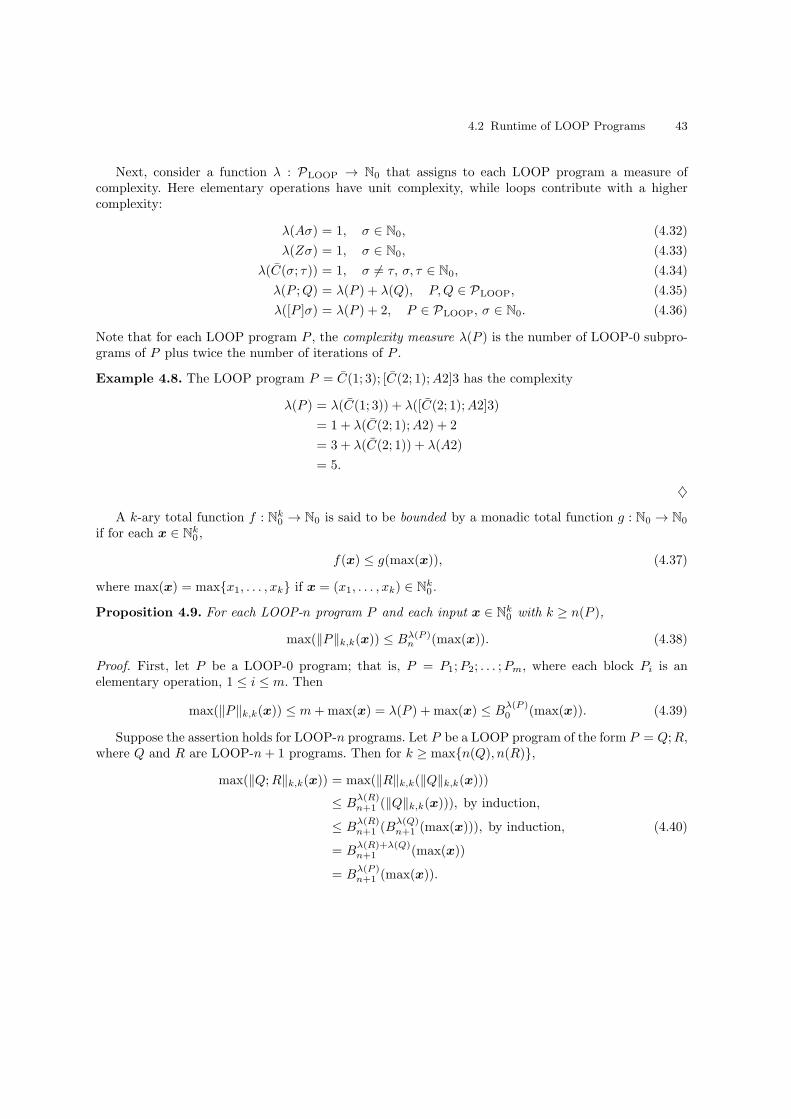
4.2 Runtime of LOOP Programs 43
Next, consider a function λ : PLOOP → N0 that assigns to each LOOP program a measure ofcomplexity. Here elementary operations have unit complexity, while loops contribute with a highercomplexity:
λ(Aσ) = 1, σ ∈ N0, (4.32)
λ(Zσ) = 1, σ ∈ N0, (4.33)
λ(C(σ; τ)) = 1, σ 6= τ, σ, τ ∈ N0, (4.34)
λ(P ;Q) = λ(P ) + λ(Q), P,Q ∈ PLOOP, (4.35)
λ([P ]σ) = λ(P ) + 2, P ∈ PLOOP, σ ∈ N0. (4.36)
Note that for each LOOP program P , the complexity measure λ(P ) is the number of LOOP-0 subpro-grams of P plus twice the number of iterations of P .
Example 4.8. The LOOP program P = C(1; 3); [C(2; 1);A2]3 has the complexity
λ(P ) = λ(C(1; 3)) + λ([C(2; 1);A2]3)
= 1 + λ(C(2; 1);A2) + 2
= 3 + λ(C(2; 1)) + λ(A2)
= 5.
♦
A k-ary total function f : Nk0 → N0 is said to be bounded by a monadic total function g : N0 → N0
if for each x ∈ Nk0 ,
f(x) ≤ g(max(x)), (4.37)
where max(x) = maxx1, . . . , xk if x = (x1, . . . , xk) ∈ Nk0 .
Proposition 4.9. For each LOOP-n program P and each input x ∈ Nk0 with k ≥ n(P ),
max(‖P‖k,k(x)) ≤ Bλ(P )n (max(x)). (4.38)
Proof. First, let P be a LOOP-0 program; that is, P = P1;P2; . . . ;Pm, where each block Pi is anelementary operation, 1 ≤ i ≤ m. Then
max(‖P‖k,k(x)) ≤ m+max(x) = λ(P ) + max(x) ≤ Bλ(P )0 (max(x)). (4.39)
Suppose the assertion holds for LOOP-n programs. Let P be a LOOP program of the form P = Q;R,where Q and R are LOOP-n+ 1 programs. Then for k ≥ maxn(Q), n(R),
max(‖Q;R‖k,k(x)) = max(‖R‖k,k(‖Q‖k,k(x)))
≤ Bλ(R)n+1 (‖Q‖k,k(x))), by induction,
≤ Bλ(R)n+1 (B
λ(Q)n+1 (max(x))), by induction, (4.40)
= Bλ(R)+λ(Q)n+1 (max(x))
= Bλ(P )n+1 (max(x)).
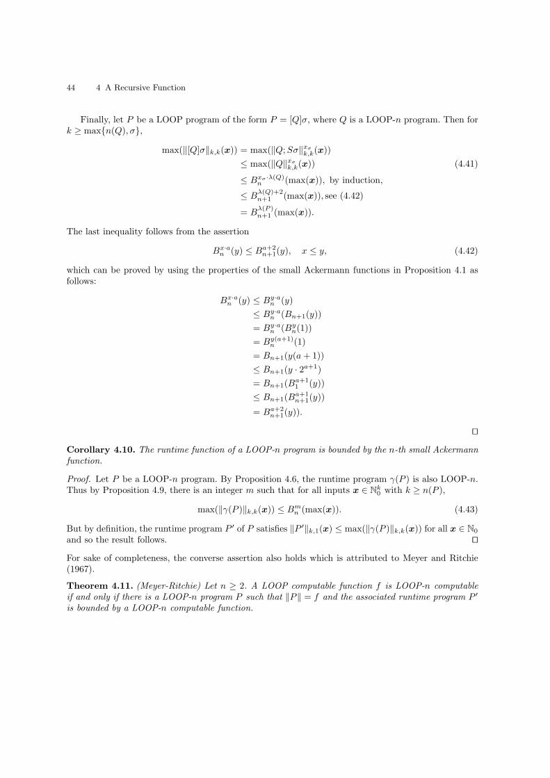
44 4 A Recursive Function
Finally, let P be a LOOP program of the form P = [Q]σ, where Q is a LOOP-n program. Then fork ≥ maxn(Q), σ,
max(‖[Q]σ‖k,k(x)) = max(‖Q;Sσ‖xσ
k,k(x))
≤ max(‖Q‖xσ
k,k(x)) (4.41)
≤ Bxσ·λ(Q)n (max(x)), by induction,
≤ Bλ(Q)+2n+1 (max(x)), see (4.42)
= Bλ(P )n+1 (max(x)).
The last inequality follows from the assertion
Bx·an (y) ≤ Ba+2n+1(y), x ≤ y, (4.42)
which can be proved by using the properties of the small Ackermann functions in Proposition 4.1 asfollows:
Bx·an (y) ≤ By·an (y)
≤ By·an (Bn+1(y))
= By·an (Byn(1))
= By(a+1)n (1)
= Bn+1(y(a+ 1))
≤ Bn+1(y · 2a+1)
= Bn+1(Ba+11 (y))
≤ Bn+1(Ba+1n+1(y))
= Ba+2n+1(y)).
⊓⊔
Corollary 4.10. The runtime function of a LOOP-n program is bounded by the n-th small Ackermannfunction.
Proof. Let P be a LOOP-n program. By Proposition 4.6, the runtime program γ(P ) is also LOOP-n.Thus by Proposition 4.9, there is an integer m such that for all inputs x ∈ N
k0 with k ≥ n(P ),
max(‖γ(P )‖k,k(x)) ≤ Bmn (max(x)). (4.43)
But by definition, the runtime program P ′ of P satisfies ‖P ′‖k,1(x) ≤ max(‖γ(P )‖k,k(x)) for all x ∈ N0
and so the result follows. ⊓⊔
For sake of completeness, the converse assertion also holds which is attributed to Meyer and Ritchie(1967).
Theorem 4.11. (Meyer-Ritchie) Let n ≥ 2. A LOOP computable function f is LOOP-n computableif and only if there is a LOOP-n program P such that ‖P‖ = f and the associated runtime program P ′
is bounded by a LOOP-n computable function.
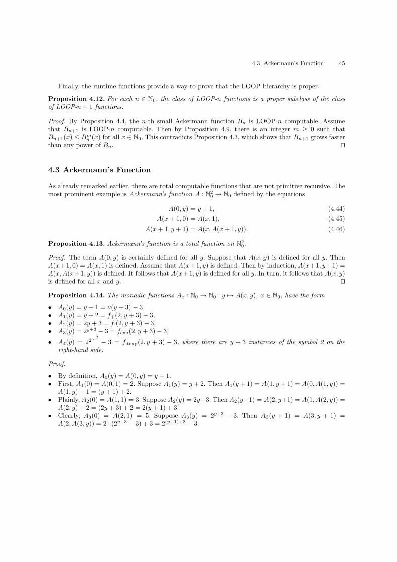
4.3 Ackermann’s Function 45
Finally, the runtime functions provide a way to prove that the LOOP hierarchy is proper.
Proposition 4.12. For each n ∈ N0, the class of LOOP-n functions is a proper subclass of the classof LOOP-n+ 1 functions.
Proof. By Proposition 4.4, the n-th small Ackermann function Bn is LOOP-n computable. Assumethat Bn+1 is LOOP-n computable. Then by Proposition 4.9, there is an integer m ≥ 0 such thatBn+1(x) ≤ B
mn (x) for all x ∈ N0. This contradicts Proposition 4.3, which shows that Bn+1 grows faster
than any power of Bn. ⊓⊔
4.3 Ackermann’s Function
As already remarked earlier, there are total computable functions that are not primitive recursive. Themost prominent example is Ackermann’s function A : N2
0 → N0 defined by the equations
A(0, y) = y + 1, (4.44)
A(x+ 1, 0) = A(x, 1), (4.45)
A(x+ 1, y + 1) = A(x,A(x+ 1, y)). (4.46)
Proposition 4.13. Ackermann’s function is a total function on N20.
Proof. The term A(0, y) is certainly defined for all y. Suppose that A(x, y) is defined for all y. ThenA(x+1, 0) = A(x, 1) is defined. Assume that A(x+1, y) is defined. Then by induction, A(x+1, y+1) =A(x,A(x+1, y)) is defined. It follows that A(x+1, y) is defined for all y. In turn, it follows that A(x, y)is defined for all x and y. ⊓⊔
Proposition 4.14. The monadic functions Ax : N0 → N0 : y 7→ A(x, y), x ∈ N0, have the form
• A0(y) = y + 1 = ν(y + 3)− 3,• A1(y) = y + 2 = f+(2, y + 3)− 3,• A2(y) = 2y + 3 = f·(2, y + 3)− 3,• A3(y) = 2y+3 − 3 = fexp(2, y + 3)− 3,
• A4(y) = 22...2
− 3 = fitexp(2, y + 3) − 3, where there are y + 3 instances of the symbol 2 on theright-hand side.
Proof.
• By definition, A0(y) = A(0, y) = y + 1.• First, A1(0) = A(0, 1) = 2. Suppose A1(y) = y + 2. Then A1(y + 1) = A(1, y + 1) = A(0, A(1, y)) =
A(1, y) + 1 = (y + 1) + 2.• Plainly, A2(0) = A(1, 1) = 3. Suppose A2(y) = 2y+3. Then A2(y+1) = A(2, y+1) = A(1, A(2, y)) =
A(2, y) + 2 = (2y + 3) + 2 = 2(y + 1) + 3.• Clearly, A3(0) = A(2, 1) = 5. Suppose A3(y) = 2y+3 − 3. Then A3(y + 1) = A(3, y + 1) =
A(2, A(3, y)) = 2 · (2y+3 − 3) + 3 = 2(y+1)+3 − 3.
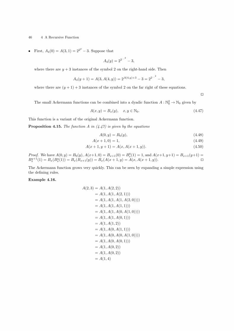
46 4 A Recursive Function
• First, A4(0) = A(3, 1) = 222
− 3. Suppose that
A4(y) = 22...2
− 3,
where there are y + 3 instances of the symbol 2 on the right-hand side. Then
A4(y + 1) = A(3, A(4, y)) = 2A(4,y)+3 − 3 = 22...2
− 3,
where there are (y + 1) + 3 instances of the symbol 2 on the far right of these equations.
⊓⊔
The small Ackermann functions can be combined into a dyadic function A : N20 → N0 given by
A(x, y) = Bx(y), x, y ∈ N0. (4.47)
This function is a variant of the original Ackermann function.
Proposition 4.15. The function A in (4.47) is given by the equations
A(0, y) = B0(y), (4.48)
A(x+ 1, 0) = 1, (4.49)
A(x+ 1, y + 1) = A(x,A(x+ 1, y)). (4.50)
Proof. We have A(0, y) = B0(y), A(x+1, 0) = Bx+1(0) = B0x(1) = 1, and A(x+1, y+1) = Bx+1(y+1) =
By+1x (1) = Bx(B
yx(1)) = Bx(Bx+1(y)) = Bx(A(x+ 1, y) = A(x,A(x+ 1, y)). ⊓⊔
The Ackermann function grows very quickly. This can be seen by expanding a simple expression usingthe defining rules.
Example 4.16.
A(2, 3) = A(1, A(2, 2))
= A(1, A(1, A(2, 1)))
= A(1, A(1, A(1, A(2, 0))))
= A(1, A(1, A(1, 1)))
= A(1, A(1, A(0, A(1, 0))))
= A(1, A(1, A(0, 1)))
= A(1, A(1, 2))
= A(1, A(0, A(1, 1)))
= A(1, A(0, A(0, A(1, 0))))
= A(1, A(0, A(0, 1)))
= A(1, A(0, 2))
= A(1, A(0, 2))
= A(1, 4)
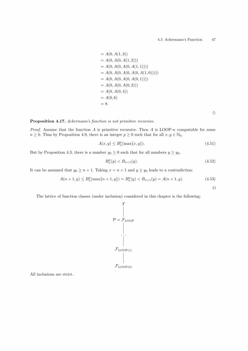
4.3 Ackermann’s Function 47
= A(0, A(1, 3))
= A(0, A(0, A(1, 2)))
= A(0, A(0, A(0, A(1, 1))))
= A(0, A(0, A(0, A(0, A(1, 0)))))
= A(0, A(0, A(0, A(0, 1))))
= A(0, A(0, A(0, 2)))
= A(0, A(0, 4))
= A(0, 6)
= 8.
♦
Proposition 4.17. Ackermann’s function is not primitive recursive.
Proof. Assume that the function A is primitive recursive. Then A is LOOP-n computable for somen ≥ 0. Thus by Proposition 4.9, there is an integer p ≥ 0 such that for all x, y ∈ N0,
A(x, y) ≤ Bpn(maxx, y). (4.51)
But by Proposition 4.3, there is a number y0 ≥ 0 such that for all numbers y ≥ y0,
Bpn(y) < Bn+1(y). (4.52)
It can be assumed that y0 ≥ n+ 1. Taking x = n+ 1 and y ≥ y0 leads to a contradiction:
A(n+ 1, y) ≤ Bpn(maxn+ 1, y) = Bpn(y) < Bn+1(y) = A(n+ 1, y). (4.53)
⊓⊔
The lattice of function classes (under inclusion) considered in this chapter is the following:
T
P = FLOOP
. . .
FLOOP(1)
FLOOP(0)
All inclusions are strict.
48 4 A Recursive Function

5
Acceptable Programming Systems
Acceptable programming systems form the basis for the development of the theory of computation. Thischapter provides several basic theoretical results of computability, such as the existence of universalfunctions, the parametrization theorem known as smn theorem, and Kleene’s normal form theorem.These results make use of the Godel numbering of partial recursive functions.
5.1 Godel Numbering of GOTO Programs
In mathematical logic, Godel numbering refers to a function that assigns to each well-formed formula ofsome formal language a unique natural number called its Godel number. This concept was introducedby the logician Kurt Godel (1906-1978) for the proof of incompleteness of elementary arithmetic (1931).Here Godel numbering is used to provide an encoding of GOTO programs.
For this, let N∗0 denote the union of all cartesian products N
k0 , k ≥ 0. In particular, N0
0 = ǫ,where ǫ is the empty string. The Cantor pairing function J2 : N2
0 → N0 is used to define an encodingJ : N∗
0 → N0 as follows:
J(ǫ) = 0, (5.1)
J(x) = J2(0, x) + 1, x ∈ N0, (5.2)
J(x, y) = J2(J(x), y) + 1, x ∈ N∗0, y ∈ N0. (5.3)
Note that the second equation is a special case of the third one, since for each y ∈ N0,
J(ǫ, y) = J2(J(ǫ), y) + 1 = J2(0, y) + 1 = J(y). (5.4)
Example 5.1. We have
J(1, 3) = J2(J(1), 3) + 1 = J2(J2(0, 1) + 1, 3) + 1 = J2(2, 3) + 1 = 17 + 1 = 18.
♦
Proposition 5.2. The encoding function J is a primitive recursive bijection.
50 5 Acceptable Programming Systems
Proof. First, claim that J is primitive recursive. Indeed, the function J is primitive recursive for stringsof length ≤ 1, since J2 is primitive recursive. Assume that J is primitive recursive for strings of length≤ k, where k ≥ 1. For strings of length k+1, the function J can be written as a composition of primitiverecursive functions:
J = ν J2(J(π(k+1)1 , . . . , π
(k+1)k ), π
(k+1)k+1 ). (5.5)
By induction hypothesis, J is primitive recursive for strings of length ≤ k+1 and thus the claim follows.Second, let A be the set of all numbers n ∈ N0 such that there is a unique string x ∈ N
∗0 with
J(x) = n. Claim that A = N0. Indeed, 0 lies in A since J(ǫ) = 0 and J(x) > 0 for all x 6= ǫ Let n > 0and assume that the assertion holds for all numbers m < n. Define
u = K2(n− 1) and v = L2(n− 1). (5.6)
Then J2(u, v) = J2(K2(n − 1), L2(n − 1)) = n − 1. By construction, K2(z) ≤ z and L2(z) ≤ z for allz ∈ N0. Thus u = K2(n − 1) < n and hence u ∈ A. By induction, there is exactly one string x ∈ N
k0
such that J(x) = u. Then J(x, v) = J2(J(x), v)) + 1 = J2(u, v) + 1 = n.Assume that J(x, v) = n = J(y, w) for some x,y ∈ N
∗0 and v, w ∈ N0. Then by definition,
J2(J(x), v) = J2(J(y), w). But the Cantor pairing function is bijective and thus J(x) = J(y) andv = w. Since J(x) < n it follows by induction that x = y. Thus n ∈ A and so by the induction axiom,A = N0. It follows that J is bijective. ⊓⊔
The encoding function J gives rise to two functions K,L : N0 → N0 defined as
K(n) = K2(n − 1) and L(n) = L2(n − 1), n ∈ N0. (5.7)
Note that the following marginal conditions hold:
K(1) = K(0) = L(0) = L(1) = 0. (5.8)
Proposition 5.3. The functions K and J are primitive recursive, and for each number n ≥ 1, thereare unique x ∈ N
∗0 and y ∈ N0 with J(x, y) = n such that
J(x) = K(n) and y = L(n). (5.9)
Proof. By Proposition 2.27, the functions K2 and L2 are primitive recursive and so K and L areprimitive recursive, too.
Let n ≥ 1. By Proposition 5.2, there are unique x ∈ N∗0 and y ∈ N0 such that J(x, y) = n. Thus
J2(J(x), y) = n−1. But J2(K2(n−1), L2(n−1)) = n−1 and the Cantor pairing function J2 is bijective.Thus K2(n− 1) = J(x) and L2(n− 1) = y, and so K(n) = J(x) and L(n) = y. ⊓⊔
The length of a string can be determined by its encoding.
Proposition 5.4. If x is a string in N∗0 of length k, then k is the smallest number such that
Kk(J(x)) = 0.
Proof. In view of the empty string, K0(J(ǫ)) = J(ǫ) = 0. Let x = x1 . . . xk be a non-empty string.Then J(x) = n ≥ 1. By Proposition 5.3, J(x1 . . . xk−1) = K(n). By induction, J(x1 . . . xi) = Kk−i(n)for each 0 ≤ i ≤ k. In particular, for each 0 ≤ i < k, Kk−i(n) is non-zero, since x1 . . . xi is not theempty string. Moreover, Kk(n) = J(ǫ) = 0. The result follows. ⊓⊔
5.1 Godel Numbering of GOTO Programs 51
Note that the converse of the above assertion is also valid. As an example, take a number x ∈ N0, a stringof length one. Then by (5.4), J(ǫ, x) = J(x) = J2(0, x) + 1 = n ≥ 1 and so by (5.9), K(n) = J(ǫ) = 0and L(n) = x.
In view of Proposition 5.4, define the mapping f : N∗0 × N0 → N0 as
f : (x, k) 7→ Kk(J(x)). (5.10)
Minimalization of this function yield the length function lg : N∗0 → N0 given by
lg(x) = µf(x) =
k if k smallest with f(x, k) = 0 and f(x, i) > 0 for 0 ≤ i ≤ k,↑ otherwise.
(5.11)
Proposition 5.5. The length function lg is primitive recursive.
Proof. The length function is partial recursive, since it is obtained by minimalization of a primitiverecursive function. But each string x has finite length and so the repeated application of K to J(x)yields 0 after a finite number of steps. Hence, the length function is total. Moreover, the length of astring x = x1 . . . xn is not larger than an upper bound of its decimal equivalent given by 10n and sothe minimalization is actually bounded. Hence, the length function is primitive recursive. ⊓⊔
Proposition 5.6. Let n ≥ 1. The inverse value J−1(n) is given by
(Kk−1(n), L Kk−2(n), . . . , L K(n), L(n)), (5.12)
where k is the smallest number such that Kk(n) = 0.
Proof. Let x ∈ N0. Then J(x) = n ≥ 1 and as shown above, K(n) = 0 and L(n) = x. Hence,J−1(n) = L(n) = x.
Let x ∈ Nk0 , k ≥ 1, and y ∈ N0. Then J(x, y) = n ≥ 1. By Proposition 5.3, K(n) = J(x) and
L(n) = y. Since K(n) < n, induction shows that x = J−1(K(n)) is given by
(Kk(n), L Kk−1(n), . . . , L K(n)).
Hence, (x, y) has the form
(Kk(n), L Kk−1(n), . . . , L K(n), L(n))
as required. ⊓⊔
The primitive recursive bijection J allows to encode the standard GOTO programs, SGOTO pro-grams for short. These are GOTO programs P = s0; s1; . . . ; sq that have a canonical labelling in thesense that λ(sl) = l, 0 ≤ l ≤ q. It is clear that for each GOTO program there is a (semantically)equivalent SGOTO program. SGOTO programs are used in the following since they will permit aslightly simpler Godel numbering than GOTO program. In the following, let PSGOTO denote the classof SGOTO programs.
Take an SGOTO program P = s0; s1; . . . ; sq. For each 0 ≤ l ≤ q, put
I(sl) =
3 · J(i− 1, k) if sl = (l, xi ← xi + 1, k),3 · J(i− 1, k) + 1 if sl = (l, xi ← xi − 1, k),3 · J(i− 1, k,m) + 2 if sl = (l, if xi = 0, k,m).
(5.13)
52 5 Acceptable Programming Systems
The number I(sl) is called the Godel number of the instruction sl, 0 ≤ l ≤ q. The function I is primitiverecursive, since it is defined by cases and the functions involved are also primitive recursive.
Note that the function I allows to identify the lth instruction of an SGOTO program given itsGodel number e. Indeed, the residue of e modulo 3 provides the type of instruction and the quotient ofe modulo 3 gives the encoding of the parameters of the instruction. More concretely, write
e = 3n+ t, (5.14)
where n = ÷(e, 3) and t = mod(e, 3). Then the instruction can be decoded by using Proposition 5.6 asfollows:
sl =
(l, xK(n)+1 ← xK(n)+1 + 1, L(n)) if t = 0,(l, xK(n)+1 ← xK(n)+1 − 1, L(n)) if t = 1,(l, if xK2(n)+1 = 0, L(K(n)), L(n)) if t = 2.
(5.15)
The Godel number of an SGOTO program P = s0; s1; . . . ; sq is defined as
Γ (P ) = J(I(s0), I(s1), . . . , I(sq)). (5.16)
Proposition 5.7. The function Γ : PSGOTO → N0 is bijective and primitive recursive.
Proof. The mapping Γ is bijective since J is bijective and the instructions encoded by I are uniquelydetermined as shown above. Moreover, the function Γ is a composition of primitive recursive functionsand thus is primitive recursive. ⊓⊔
The SGOTO program P with Godel number e is denoted by Pe. This Godel numbering provides alist of all SGOTO programs
P0, P1, P2, . . . . (5.17)
Conversely, each number e can be assigned the SGOTO program P such that Γ (P ) = e. For this, thelength of the string encoded by e is first determined by the minimalization given in Proposition 5.4.Suppose the string has length n + 1, where n ≥ 0. Then the task is to find x ∈ N
n0 and y ∈ N0 such
that J(x, y) = n. But by (5.9), K(n) = J(x) and L(n) = y and so the preimage of n under J can berepeatedly determined. Finally, when the string is given, the preimage (instruction) of each number isestablished as described in (5.15).
For each number e and each number n ≥ 0, denote the n-ary partial recursive function computingthe SGOTO program with Godel number e by
φ(n)e = ‖Pe‖n,1. (5.18)
If f is an n-ary partial recursive function, each number e ∈ N0 with the property f = φ(n)e is called
an index of f . The index of a partial recursive function f provides the Godel number of an SGOTOprogram computing it. The list of all SGOTO program in (5.17) yiels a list of all n-ary partial recursivefunctions:
φ(n)0 , φ
(n)1 , φ
(n)2 , . . . . (5.19)
Note that the list contain repetitions, since each n-ary partial recursive function has infinitely manyindices.
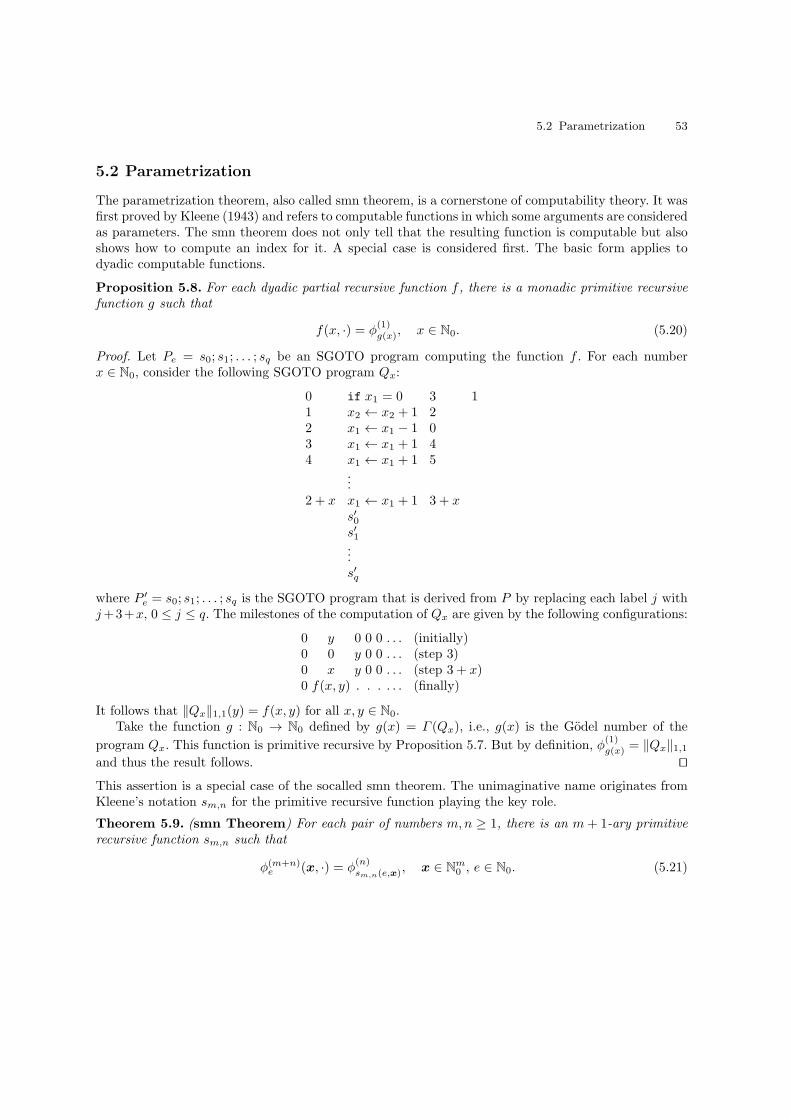
5.2 Parametrization 53
5.2 Parametrization
The parametrization theorem, also called smn theorem, is a cornerstone of computability theory. It wasfirst proved by Kleene (1943) and refers to computable functions in which some arguments are consideredas parameters. The smn theorem does not only tell that the resulting function is computable but alsoshows how to compute an index for it. A special case is considered first. The basic form applies todyadic computable functions.
Proposition 5.8. For each dyadic partial recursive function f , there is a monadic primitive recursivefunction g such that
f(x, ·) = φ(1)g(x), x ∈ N0. (5.20)
Proof. Let Pe = s0; s1; . . . ; sq be an SGOTO program computing the function f . For each numberx ∈ N0, consider the following SGOTO program Qx:
0 if x1 = 0 3 11 x2 ← x2 + 1 22 x1 ← x1 − 1 03 x1 ← x1 + 1 44 x1 ← x1 + 1 5
...2 + x x1 ← x1 + 1 3 + x
s′0s′1...s′q
where P ′e = s0; s1; . . . ; sq is the SGOTO program that is derived from P by replacing each label j with
j+3+x, 0 ≤ j ≤ q. The milestones of the computation of Qx are given by the following configurations:
0 y 0 0 0 . . . (initially)0 0 y 0 0 . . . (step 3)0 x y 0 0 . . . (step 3 + x)0 f(x, y) . . . . . . (finally)
It follows that ‖Qx‖1,1(y) = f(x, y) for all x, y ∈ N0.Take the function g : N0 → N0 defined by g(x) = Γ (Qx), i.e., g(x) is the Godel number of the
program Qx. This function is primitive recursive by Proposition 5.7. But by definition, φ(1)g(x) = ‖Qx‖1,1
and thus the result follows. ⊓⊔
This assertion is a special case of the socalled smn theorem. The unimaginative name originates fromKleene’s notation sm,n for the primitive recursive function playing the key role.
Theorem 5.9. (smn Theorem) For each pair of numbers m,n ≥ 1, there is an m+ 1-ary primitiverecursive function sm,n such that
φ(m+n)e (x, ·) = φ
(n)sm,n(e,x)
, x ∈ Nm0 , e ∈ N0. (5.21)
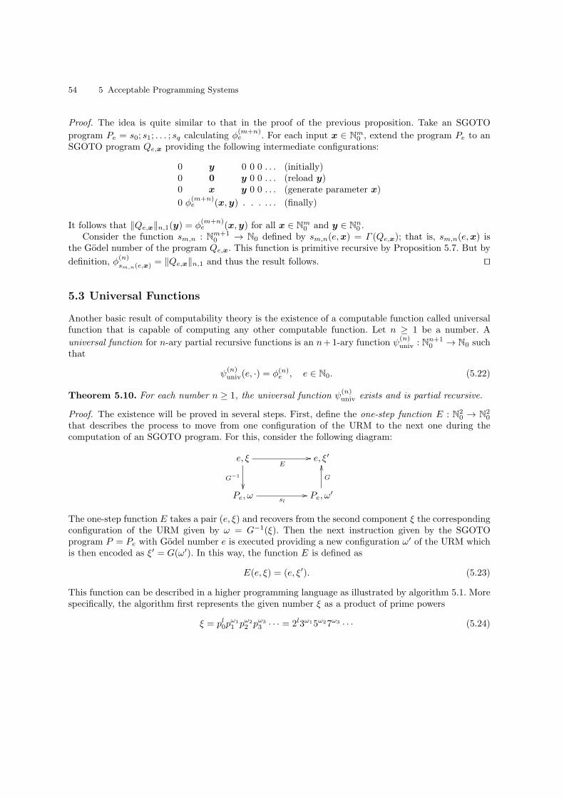
54 5 Acceptable Programming Systems
Proof. The idea is quite similar to that in the proof of the previous proposition. Take an SGOTO
program Pe = s0; s1; . . . ; sq calculating φ(m+n)e . For each input x ∈ N
m0 , extend the program Pe to an
SGOTO program Qe,x providing the following intermediate configurations:
0 y 0 0 0 . . . (initially)0 0 y 0 0 . . . (reload y)0 x y 0 0 . . . (generate parameter x)
0 φ(m+n)e (x,y) . . . . . . (finally)
It follows that ‖Qe,x‖n,1(y) = φ(m+n)e (x,y) for all x ∈ N
m0 and y ∈ N
n0 .
Consider the function sm,n : Nm+10 → N0 defined by sm,n(e,x) = Γ (Qe,x); that is, sm,n(e,x) is
the Godel number of the program Qe,x. This function is primitive recursive by Proposition 5.7. But by
definition, φ(n)sm,n(e,x)
= ‖Qe,x‖n,1 and thus the result follows. ⊓⊔
5.3 Universal Functions
Another basic result of computability theory is the existence of a computable function called universalfunction that is capable of computing any other computable function. Let n ≥ 1 be a number. A
universal function for n-ary partial recursive functions is an n+1-ary function ψ(n)univ : Nn+1
0 → N0 suchthat
ψ(n)univ(e, ·) = φ(n)e , e ∈ N0. (5.22)
Theorem 5.10. For each number n ≥ 1, the universal function ψ(n)univ exists and is partial recursive.
Proof. The existence will be proved in several steps. First, define the one-step function E : N20 → N
20
that describes the process to move from one configuration of the URM to the next one during thecomputation of an SGOTO program. For this, consider the following diagram:
e, ξE
//
G−1
e, ξ′
Pe, ω sl// Pe, ω′
G
OO
The one-step function E takes a pair (e, ξ) and recovers from the second component ξ the correspondingconfiguration of the URM given by ω = G−1(ξ). Then the next instruction given by the SGOTOprogram P = Pe with Godel number e is executed providing a new configuration ω′ of the URM whichis then encoded as ξ′ = G(ω′). In this way, the function E is defined as
E(e, ξ) = (e, ξ′). (5.23)
This function can be described in a higher programming language as illustrated by algorithm 5.1. Morespecifically, the algorithm first represents the given number ξ as a product of prime powers
ξ = pl0pω11 pω2
2 pω33 · · · = 2l3ω15ω27ω3 · · · (5.24)
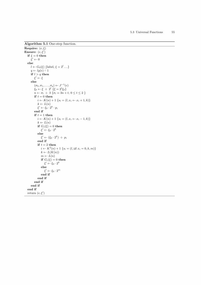
5.3 Universal Functions 55
Algorithm 5.1 One-step function.
Require: (e, ξ)Ensure: (e, ξ′)
if ξ = 0 then
ξ′ ← 0else
l← G0(ξ) label, ξ = 2l . . .q ← lg(e) − 1if l > q then
ξ′ ← ξ
else
(σ0, σ1, . . . , σq)← J−1(e)ξ0 ← ξ ÷ 2l ξ = 2lξ0n← σl ÷ 3 σl = 3n+ t, 0 ≤ t ≤ 2 if t = 0 then
i← K(n) + 1 sl = (l, xi ← xi + 1, k)k ← L(n)ξ′ ← ξ0 · 2
k · piend if
if t = 1 then
i← K(n) + 1 sl = (l, xi ← xi − 1, k)k ← L(n)if Gi(ξ) = 0 then
ξ′ ← ξ0 · 2k
else
ξ′ ← (ξ0 · 2k) ÷ pi
end if
if t = 2 then
i← K2(n) + 1 sl = (l, if xi = 0, k,m)k ← L(K(n))m← L(n)if Gi(ξ) = 0 then
ξ′ ← ξ0 · 2k
else
ξ′ ← ξ0 · 2m
end if
end if
end if
end if
end if
return (e, ξ′)
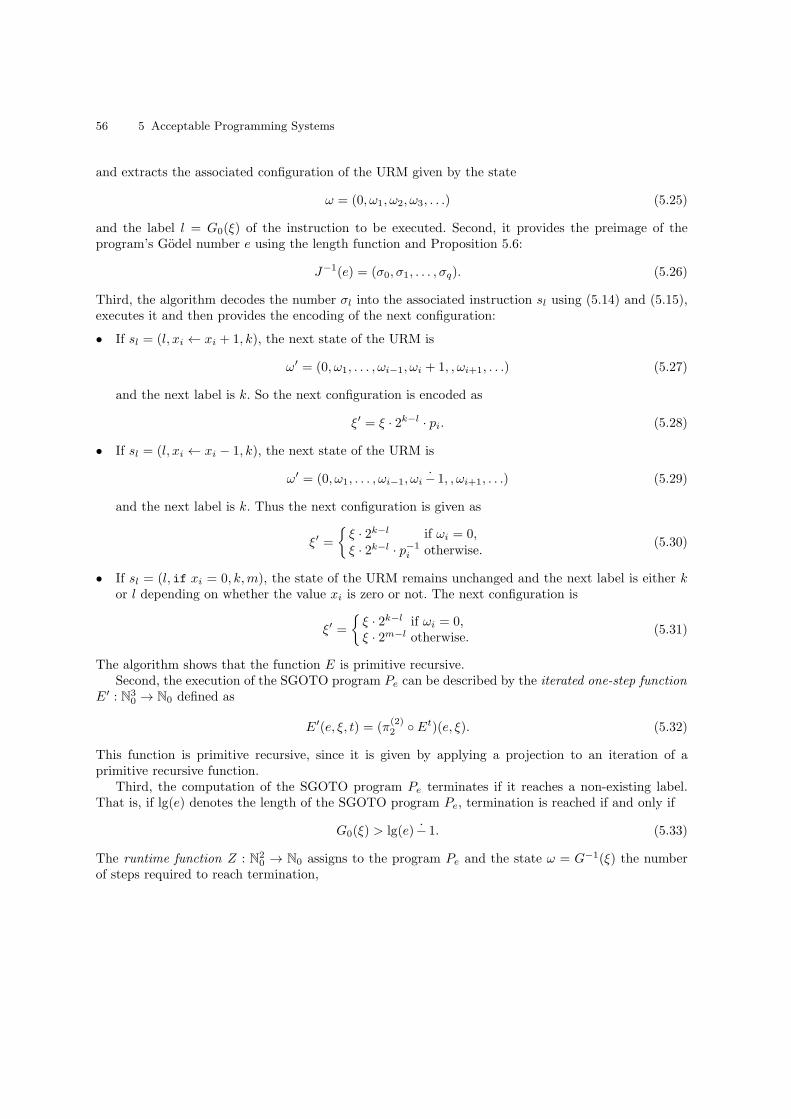
56 5 Acceptable Programming Systems
and extracts the associated configuration of the URM given by the state
ω = (0, ω1, ω2, ω3, . . .) (5.25)
and the label l = G0(ξ) of the instruction to be executed. Second, it provides the preimage of theprogram’s Godel number e using the length function and Proposition 5.6:
J−1(e) = (σ0, σ1, . . . , σq). (5.26)
Third, the algorithm decodes the number σl into the associated instruction sl using (5.14) and (5.15),executes it and then provides the encoding of the next configuration:
• If sl = (l, xi ← xi + 1, k), the next state of the URM is
ω′ = (0, ω1, . . . , ωi−1, ωi + 1, , ωi+1, . . .) (5.27)
and the next label is k. So the next configuration is encoded as
ξ′ = ξ · 2k−l · pi. (5.28)
• If sl = (l, xi ← xi − 1, k), the next state of the URM is
ω′ = (0, ω1, . . . , ωi−1, ωi − 1, , ωi+1, . . .) (5.29)
and the next label is k. Thus the next configuration is given as
ξ′ =
ξ · 2k−l if ωi = 0,ξ · 2k−l · p−1
i otherwise.(5.30)
• If sl = (l, if xi = 0, k,m), the state of the URM remains unchanged and the next label is either kor l depending on whether the value xi is zero or not. The next configuration is
ξ′ =
ξ · 2k−l if ωi = 0,ξ · 2m−l otherwise.
(5.31)
The algorithm shows that the function E is primitive recursive.Second, the execution of the SGOTO program Pe can be described by the iterated one-step function
E′ : N30 → N0 defined as
E′(e, ξ, t) = (π(2)2 E
t)(e, ξ). (5.32)
This function is primitive recursive, since it is given by applying a projection to an iteration of aprimitive recursive function.
Third, the computation of the SGOTO program Pe terminates if it reaches a non-existing label.That is, if lg(e) denotes the length of the SGOTO program Pe, termination is reached if and only if
G0(ξ) > lg(e) − 1. (5.33)
The runtime function Z : N20 → N0 assigns to the program Pe and the state ω = G−1(ξ) the number
of steps required to reach termination,
5.4 Kleene’s Normal Form 57
Z(e, ξ) = µt(csg(G0(E′(e, ξ, t)) − (lg(e) − 1))), (5.34)
where the minimalization µ = µt is subject to the variable t counting the number of steps. This functionis only partial recursive since the minimalization is unbounded, i.e., the program Pe may not terminate.
Fourth, the residual step function is defined by the partial function R : N20 → N0 which assigns to
each SGOTO program Pe and each initial state ω = G−1(ξ) the result of computation given by thecontent of the first register:
R(e, ξ) = G1(E′(e, ξ, Z(e, ξ))). (5.35)
This function is partial recursive, since the function Z is partial recursive.Summing up, the desired partial recursive function is given as
ψ(n)univ(e,x) = φ(n)e (x) = ‖Pe‖n,1(x) = R(e,G(0, x1, . . . , xn, 0, 0, . . .)), (5.36)
where e is a Godel number and x = (x1, . . . , xn) ∈ Nn0 an input. ⊓⊔
The existence of universal functions implies the existence of universal URM programs, and vice versa.An acceptable programming system is considered to be an enumeration of n-ary partial recursive
functions ψ0, ψ1, ψ2, . . . for which both the smn theorem and the theorem for universal function hold. Forinstance, the enumeration of URM (or GOTO) computable functions forms an acceptable programmingsystem.
5.4 Kleene’s Normal Form
Kleene (1943) introduced the T predicate that tells whether an SGOTO program will halt when runwith a particular input and if so, a corresponding function provides the result of computation. Similarto the smn theorem, the original notation used by Kleene has become standard terminology.
First note that the definition of the universal function allows to define the Kleene set Sn ⊆ Nn+30 ,
n ≥ 1, given as
(e,x, z, t) ∈ Sn :⇐⇒ csg[G0(E′(e, ξx, t)) − (lg(e) − 1)] = 0 ∧ G1(E
′(e, ξx, t)) = z, (5.37)
where ξx = (0, x1, . . . , xn, 0, 0, . . .) is the initial state comprising the input x = (x1, . . . , xn) ∈ Nn0 .
Clearly, (e,x, z, t) ∈ Sn if and only if the program φe with input x terminates after t steps with theresult z. The set Sn is primitive recursive since the number of steps is explicitly given.
Let A ⊆ Nn+10 be a relation. First, the unbounded minimalization of A is the function µA : Nn0 → N0
defined as
µA(x) = µ(csg χA)(x) =
y if (x, y) ∈ A and (x, i) 6∈ A for all 0 ≤ i < y,↑ otherwise.
(5.38)
We write
µA(x) = µy[(x, y) ∈ A], x ∈ Nn0 . (5.39)
Second, the unbounded existential quantification of A is the relation EA ⊆ Nn0 given by
58 5 Acceptable Programming Systems
EA = x | ∃y ∈ N0 : (x, y) ∈ A. (5.40)
Put
∃y[(x, y) ∈ A] :⇐⇒ x ∈ EA, x ∈ Nn0 . (5.41)
Third, the unbounded universal quantification of A is the relation UA ⊆ Nn0 defined by
UA = x | ∀y ∈ N0 : (x, y) ∈ A. (5.42)
Set
∀y[(x, y) ∈ A] :⇐⇒ x ∈ EA, x ∈ Nn0 . (5.43)
Theorem 5.11. (Kleene) For each number n ≥ 1, there is a primitive recursive set Tn ⊆ Nn+20 called
Kleene predicate such that for all x ∈ Nn0 :
x ∈ domφ(n)e ⇐⇒ (e,x) ∈ ∃y[(e,x, y) ∈ Tn]. (5.44)
If x ∈ domφ(n)e , there is a primitive recursive function U : N0 → N0 such that
φ(n)e (x) = U(µy[(e,x, y) ∈ Tn]). (5.45)
Proof. Define the relation Tn ⊆ Nn+20 as follows:
(e,x, y) ∈ Tn :⇐⇒ (e,x,K2(y), L2(y)) ∈ Sn. (5.46)
That is, the component y encodes both, the result of computation z = K2(y) and the number of stepst = L2(y). Since the relation Sn and the functions K2 and L2 are primitive recursive, it follows thatthe relation Tn is primitive recursive, too.
Let x ∈ Nn0 lie in the domain of φ
(n)e and let φ
(n)e (x) = z. Then there is a number t ≥ 0 such that
(e,x, z, t) ∈ Sn. Putting y = J2(z, t) yields (e,x, y) ∈ Tn; that is, (e,x) ∈ ∃y[(e,x, y) ∈ Tn].Conversely, let (e,x) ∈ ∃y[(e,x, y) ∈ Tn] and let y ≥ 0 be a number such that (e,x, y) ∈ Tn. Then
by definition, (e,x,K2(y), L2(y)) ∈ Sn and hence x belongs to the domain of φ(n)e .
Finally, let x ∈ domφ(n)e . Then there is a number y ≥ 0 such that (e,x, y) ∈ Tn. Define the function
U : N0 → N0 by putting U(y) = K2(y). The function U is primitive recursive and by definition of Snyields the result of computation. ⊓⊔
Kleene’s normal form implies that any partial recursive function can be defined by using a singleinstance of the µ (minimalization) operator applied to a primitive recursive function. In the context ofprogramming, this means that any program can be written with a single while loop.
6
Turing Machine
The Turing machine was described by the British mathematician Alan Turing (1912-1954) in 1937 asa thought experiment representing a computing machine. Despite its simplicity, a Turing machine is auniversal device of computation.
6.1 The Machinery
A Turing machine consists of an infinite tape and an associated read/write head connected to a controlmechanism. The tape is divided into denumerably many cells, each of which containing a symbol froma tape alphabet. This alphabet contains the special symbol ”b” signifying that a cell is blank or empty.The cells are scanned, one at a time, by the read/write head which is able to move in both directions.At any given time instant, the machine will be in one of a finite number of states. The behaviour ofthe read/write head and the change of the machine’s state are governed by the present state of themachine and by the symbol in the cell under scan.
The machine operates on words over an input alphabet. The symbols forming a word are written, inorder, in consecutive cells of the tape from left to right. When the machine enters a state, the read/writehead scans the symbol in the controlled cell, and writes in this cell a symbol from the tape alphabet;it then moves one cell to the left, or one cell to the right, or not at all; after that, the machine enters anew state.
A Turing machine is a quintuple M = (Σ,Q, T, q0, qF ) consisting of
• a finite alphabet Σ, called tape alphabet, containing a distinguished blank symbol b; the subsetΣI = Σ \ b is called input alphabet.
• a finite set Q of states,• a partial function T : Q×Σ → Q×Σ × L,R,Λ, the state transition function,• a start state q0 ∈ Q, and• a halt state qF ∈ Q such that T (qF , σ) is undefined for all σ in Σ.
The symbols L, R, and Λ are interpreted as left move, right move, and no move, respectively. The tapecells can be numbered by the set of integers Z, and the tape contents can be considered as a mappingτ : Z → Σ which assigns blank to almost every cell; that is, only a finite portion of the tape containssymbols from the input alphabet.
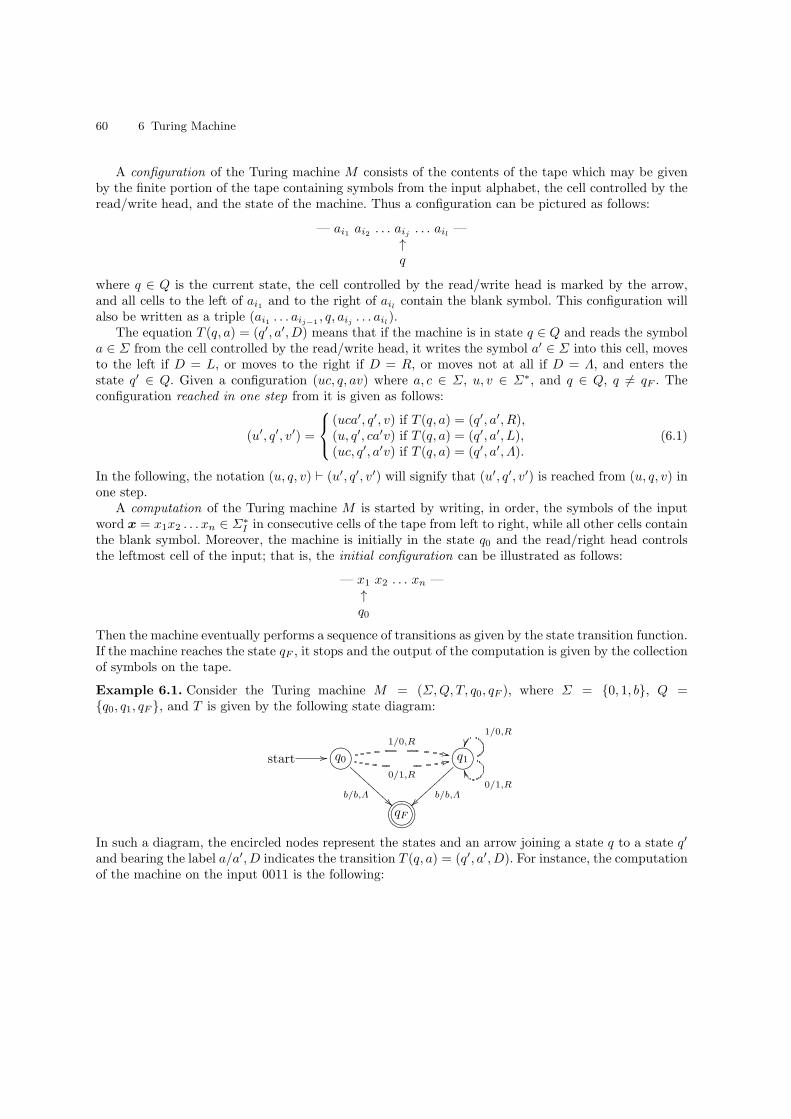
60 6 Turing Machine
A configuration of the Turing machine M consists of the contents of the tape which may be givenby the finite portion of the tape containing symbols from the input alphabet, the cell controlled by theread/write head, and the state of the machine. Thus a configuration can be pictured as follows:
— ai1 ai2 . . . aij . . . ail —↑q
where q ∈ Q is the current state, the cell controlled by the read/write head is marked by the arrow,and all cells to the left of ai1 and to the right of ail contain the blank symbol. This configuration willalso be written as a triple (ai1 . . . aij−1
, q, aij . . . ail).The equation T (q, a) = (q′, a′, D) means that if the machine is in state q ∈ Q and reads the symbol
a ∈ Σ from the cell controlled by the read/write head, it writes the symbol a′ ∈ Σ into this cell, movesto the left if D = L, or moves to the right if D = R, or moves not at all if D = Λ, and enters thestate q′ ∈ Q. Given a configuration (uc, q, av) where a, c ∈ Σ, u, v ∈ Σ∗, and q ∈ Q, q 6= qF . Theconfiguration reached in one step from it is given as follows:
(u′, q′, v′) =
(uca′, q′, v) if T (q, a) = (q′, a′, R),(u, q′, ca′v) if T (q, a) = (q′, a′, L),(uc, q′, a′v) if T (q, a) = (q′, a′, Λ).
(6.1)
In the following, the notation (u, q, v) ⊢ (u′, q′, v′) will signify that (u′, q′, v′) is reached from (u, q, v) inone step.
A computation of the Turing machine M is started by writing, in order, the symbols of the inputword x = x1x2 . . . xn ∈ Σ
∗I in consecutive cells of the tape from left to right, while all other cells contain
the blank symbol. Moreover, the machine is initially in the state q0 and the read/right head controlsthe leftmost cell of the input; that is, the initial configuration can be illustrated as follows:
— x1 x2 . . . xn —↑q0
Then the machine eventually performs a sequence of transitions as given by the state transition function.If the machine reaches the state qF , it stops and the output of the computation is given by the collectionof symbols on the tape.
Example 6.1. Consider the Turing machine M = (Σ,Q, T, q0, qF ), where Σ = 0, 1, b, Q =q0, q1, qF , and T is given by the following state diagram:
start // ?>=<89:;q0
1/0,R,,
0/1,R
22
b/b,Λ B
BBBB
BBBB
?>=<89:;q1
1/0,R
0/1,R
TT
b/b,Λ~~|||||||||
GFED@ABC?>=<89:;qF
In such a diagram, the encircled nodes represent the states and an arrow joining a state q to a state q′
and bearing the label a/a′, D indicates the transition T (q, a) = (q′, a′, D). For instance, the computationof the machine on the input 0011 is the following:
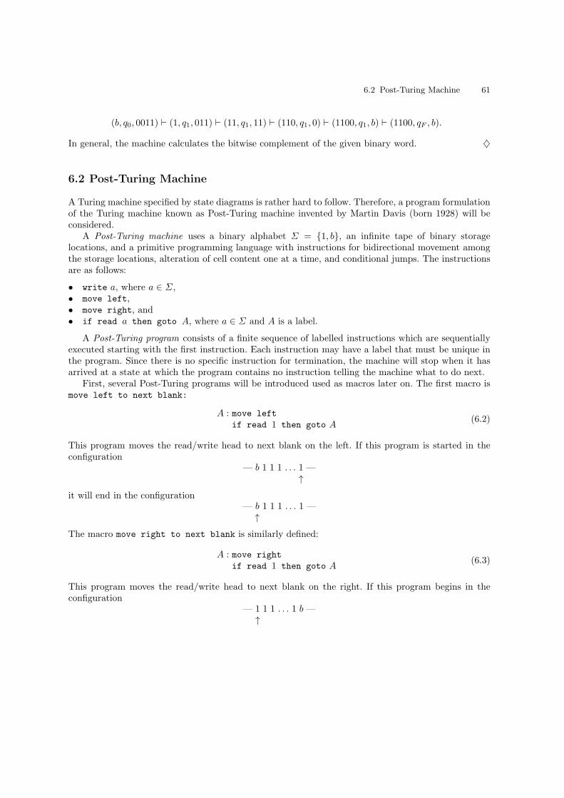
6.2 Post-Turing Machine 61
(b, q0, 0011) ⊢ (1, q1, 011) ⊢ (11, q1, 11) ⊢ (110, q1, 0) ⊢ (1100, q1, b) ⊢ (1100, qF , b).
In general, the machine calculates the bitwise complement of the given binary word. ♦
6.2 Post-Turing Machine
A Turing machine specified by state diagrams is rather hard to follow. Therefore, a program formulationof the Turing machine known as Post-Turing machine invented by Martin Davis (born 1928) will beconsidered.
A Post-Turing machine uses a binary alphabet Σ = 1, b, an infinite tape of binary storagelocations, and a primitive programming language with instructions for bidirectional movement amongthe storage locations, alteration of cell content one at a time, and conditional jumps. The instructionsare as follows:
• write a, where a ∈ Σ,• move left,• move right, and• if read a then goto A, where a ∈ Σ and A is a label.
A Post-Turing program consists of a finite sequence of labelled instructions which are sequentiallyexecuted starting with the first instruction. Each instruction may have a label that must be unique inthe program. Since there is no specific instruction for termination, the machine will stop when it hasarrived at a state at which the program contains no instruction telling the machine what to do next.
First, several Post-Turing programs will be introduced used as macros later on. The first macro ismove left to next blank:
A : move left
if read 1 then goto A(6.2)
This program moves the read/write head to next blank on the left. If this program is started in theconfiguration
— b 1 1 1 . . . 1 —↑
it will end in the configuration— b 1 1 1 . . . 1 —↑
The macro move right to next blank is similarly defined:
A : move right
if read 1 then goto A(6.3)
This program moves the read/write head to next blank on the right. If this program begins in theconfiguration
— 1 1 1 . . . 1 b —↑
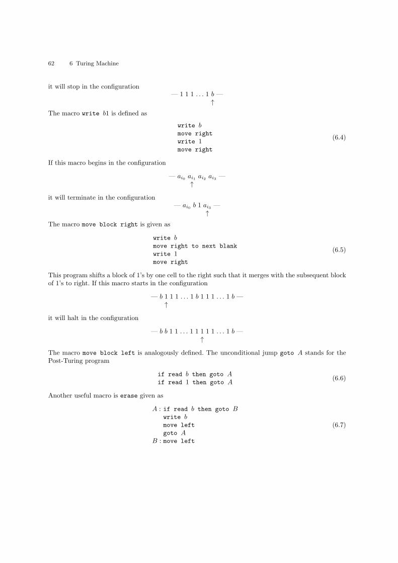
62 6 Turing Machine
it will stop in the configuration— 1 1 1 . . . 1 b —
↑
The macro write b1 is defined as
write bmove right
write 1move right
(6.4)
If this macro begins in the configuration
— ai0 ai1 ai2 ai3 —↑
it will terminate in the configuration— ai0 b 1 ai3 —
↑
The macro move block right is given as
write bmove right to next blank
write 1move right
(6.5)
This program shifts a block of 1’s by one cell to the right such that it merges with the subsequent blockof 1’s to right. If this macro starts in the configuration
— b 1 1 1 . . . 1 b 1 1 1 . . . 1 b —↑
it will halt in the configuration
— b b 1 1 . . . 1 1 1 1 1 . . . 1 b —↑
The macro move block left is analogously defined. The unconditional jump goto A stands for thePost-Turing program
if read b then goto Aif read 1 then goto A
(6.6)
Another useful macro is erase given as
A : if read b then goto Bwrite bmove left
goto AB : move left
(6.7)

6.3 Turing Computable Functions 63
This program deletes a block of 1’s from right to left. If it starts in the configuration
— a b 1 1 1 . . . 1 b —↑
where a is an arbitrary symbol, it will stop in the configuration
— a b b b b . . . b b —↑
Finally, the repetition of a statement such as
move left
move left
move left
(6.8)
will be abbreviated by denoting the statement and the number of repetitions in parenthesis such as
move left (3) (6.9)
For instance, the routine move block right (2) shifts two consecutive blocks by one cell to the right.It turns the configuration
— b 1 1 . . . 1 b 1 1 . . . 1 b 1 1 . . . 1 b —↑
into the configuration— b b 1 . . . 1 1 b 1 . . . 1 1 1 1 . . . 1 b —
↑
6.3 Turing Computable Functions
The Turing machine has the same computational capabilities as the unrestricted register machine.To prove this, it will be shown that the URM computable functions are computable by Post-Turingprograms. For this, let f : Nk0 → N0 be an URM computable function. It may be assumed that thereis a GOTO program P that computes the function f and uses the variables x1, . . . , xn, where n ≥ k.The goal is to provide a Post-Turing program P ′ that simulates the computation of P . The programP ′ consists of three subroutines:
start: initiatesimulate
clean up
(6.10)
The routine initiate presets the program for the computation of the function f . An input x =(x1, . . . , xk) ∈ N
k0 of the function f is encoded on the tape in unary format; that is, a natural number
x is represented by a block of x + 1 ones and a sequence of k numbers is described by k blocks suchthat consecutive blocks are separated by one blank. Thus the initial tape looks as follows:
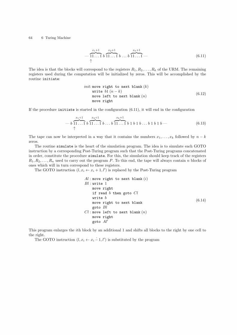
64 6 Turing Machine
—
x1+1︷ ︸︸ ︷
11 . . . 1 b
x2+1︷ ︸︸ ︷
11 . . . 1 b . . . b
xk+1︷ ︸︸ ︷
11 . . . 1 —↑
(6.11)
The idea is that the blocks will correspond to the registers R1, R2, . . . , Rk of the URM. The remainingregisters used during the computation will be initialized by zeros. This will be accomplished by theroutine initiate:
init: move right to next blank (k)write b1 (n− k)move left to next blank (n)move right
(6.12)
If the procedure initiate is started in the configuration (6.11), it will end in the configuration
— b
x1+1︷ ︸︸ ︷
11 . . . 1 b
x2+1︷ ︸︸ ︷
11 . . . 1 b . . . b
xk+1︷ ︸︸ ︷
11 . . . 1 b 1 b 1 b . . . b 1 b 1 b —↑
(6.13)
The tape can now be interpreted in a way that it contains the numbers x1, . . . , xk followed by n − kzeros.
The routine simulate is the heart of the simulation program. The idea is to simulate each GOTOinstruction by a corresponding Post-Turing program such that the Post-Turing programs concatenatedin order, constitute the procedure simulate. For this, the simulation should keep track of the registersR1, R2, . . . , Rn used to carry out the program P . To this end, the tape will always contain n blocks ofones which will in turn correspond to these registers.
The GOTO instruction (l, xi ← xi + 1, l′) is replaced by the Post-Turing program
Al : move right to next blank (i)Bl : write 1
move right
if read b then goto Clwrite bmove right to next blank
goto BlCl : move left to next blank (n)
move right
goto Al′
(6.14)
This program enlarges the ith block by an additional 1 and shifts all blocks to the right by one cell tothe right.
The GOTO instruction (l, xi ← xi − 1, l′) is substituted by the program

6.3 Turing Computable Functions 65
Al : move right to next blank (i)move left (2)if read 1 then goto Blgoto Cl
Bl : move left to next blank (i)move right
move block right (i− 1)write bmove left to next blank (i− 1)move right
goto Al′
Cl : move left to next blank (i− 1)move right
goto Al′
(6.15)
This subroutine shortens the ith block by a single 1 if it contains at least two 1’s which corresponds toa non-zero number; otherwise, the block is left invariant. Then all blocks to the left are shifted by onecell to the right.
The GOTO instruction (l, if xi = 0, l′, l′′) is superseded by the program
Al : move right to next blank (i)move left (2)if read 1 then goto Blgoto Cl
Bl : move left to next blank (i)move right
goto Al′′
Cl : move left to next blank (i− 1)move right
goto Al′
(6.16)
This program checks if the ith block contains one or more 1’s and jumps accordingly to the label Al′
or Al′′.Note that when one of these subroutines ends, the read/write head always points to the first cell of
the first block.Suppose the routine simulate starts with the configuration (6.11) and terminates; this will exactly
be the case when the input x = (x1, . . . , xk) belongs to the domain of the function f . In this case, thetape will contain in the first block the unary encoding of the result f(x):
— b
f(x)+1︷ ︸︸ ︷
11 . . . 1 b
y2+1︷ ︸︸ ︷
11 . . . 1 b . . . b
yn+1︷ ︸︸ ︷
11 . . . 1 b —↑
(6.17)
Finally, the subroutine clean up will rectify the tape such that upon termination the tape will onlycontain f(x) ones. This will be achieved by the code
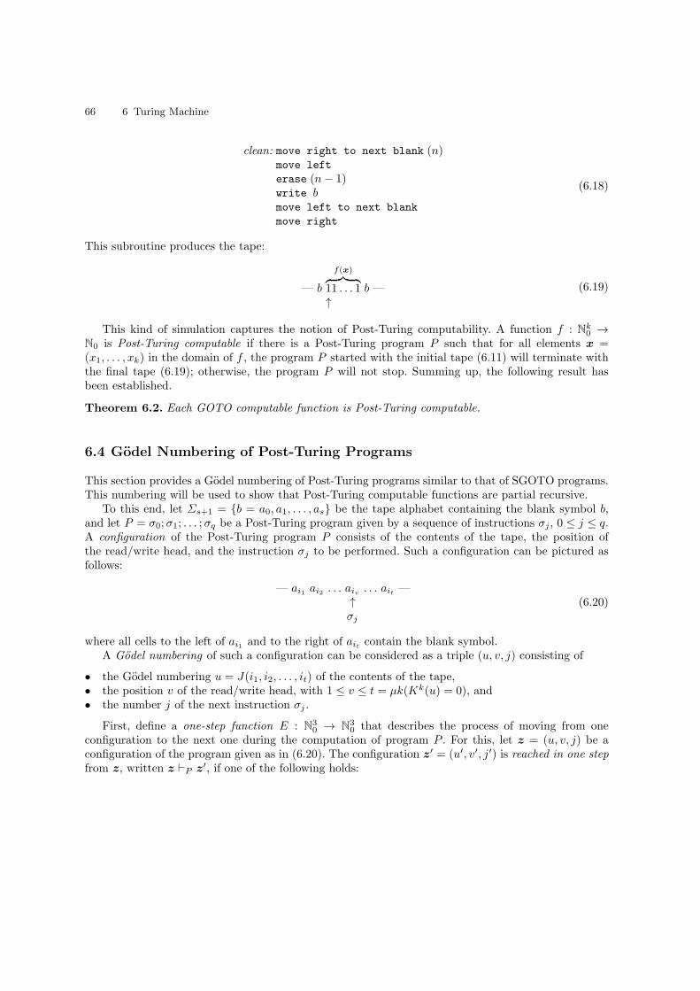
66 6 Turing Machine
clean: move right to next blank (n)move left
erase (n− 1)write bmove left to next blank
move right
(6.18)
This subroutine produces the tape:
— b
f(x)︷ ︸︸ ︷
11 . . . 1 b —↑
(6.19)
This kind of simulation captures the notion of Post-Turing computability. A function f : Nk0 →N0 is Post-Turing computable if there is a Post-Turing program P such that for all elements x =(x1, . . . , xk) in the domain of f , the program P started with the initial tape (6.11) will terminate withthe final tape (6.19); otherwise, the program P will not stop. Summing up, the following result hasbeen established.
Theorem 6.2. Each GOTO computable function is Post-Turing computable.
6.4 Godel Numbering of Post-Turing Programs
This section provides a Godel numbering of Post-Turing programs similar to that of SGOTO programs.This numbering will be used to show that Post-Turing computable functions are partial recursive.
To this end, let Σs+1 = b = a0, a1, . . . , as be the tape alphabet containing the blank symbol b,and let P = σ0;σ1; . . . ;σq be a Post-Turing program given by a sequence of instructions σj , 0 ≤ j ≤ q.A configuration of the Post-Turing program P consists of the contents of the tape, the position ofthe read/write head, and the instruction σj to be performed. Such a configuration can be pictured asfollows:
— ai1 ai2 . . . aiv . . . ait —↑σj
(6.20)
where all cells to the left of ai1 and to the right of ait contain the blank symbol.A Godel numbering of such a configuration can be considered as a triple (u, v, j) consisting of
• the Godel numbering u = J(i1, i2, . . . , it) of the contents of the tape,• the position v of the read/write head, with 1 ≤ v ≤ t = µk(Kk(u) = 0), and• the number j of the next instruction σj .
First, define a one-step function E : N30 → N
30 that describes the process of moving from one
configuration to the next one during the computation of program P . For this, let z = (u, v, j) be aconfiguration of the program given as in (6.20). The configuration z′ = (u′, v′, j′) is reached in one stepfrom z, written z ⊢P z′, if one of the following holds:
6.4 Godel Numbering of Post-Turing Programs 67
• If σj is write ai,
(u′, v′, j′) = (J(i1, . . . , iv−1, i, iv+1, . . . , it), v, j + 1). (6.21)
• If σj is move left,
(u′, v′, j′) =
(u, v − 1, j + 1) if v > 1,(J(0, i1, . . . , it), v, j + 1) otherwise.
(6.22)
• If σj is move right,
(u′, v′, j′) =
(u, v + 1, j + 1) if v < µk(Kk(u) = 0),(J(i1, . . . , it, 0), v + 1, j + 1) otherwise.
(6.23)
• If σj is if read ai then goto A, where the label A is given as an instruction number,
(u′, v′, j′) =
(u, v,A) if iv[= L(Kt−v(u)] = i,(u, v, j + 1) otherwise.
(6.24)
The function E : z 7→ z′ is defined by cases and primitive recursive operations. It follows that E isprimitive recursive.
Second, the execution of the GOTO program P is given by a sequence z0, z1, z2, . . . of configurationssuch that zi ⊢P zi+1 for each i ≥ 0. During this process, a configuration zt may eventually be reachedsuch that the label of the involved instruction does not belong to the set of instruction numbersL(P ) = 0, 1, . . . , q. In this case, the program P terminates. Such an event may eventually not happen.In this way, the runtime function of P is a partial function ZP : N3
0 → N0 given by
ZP : z 7→
mint ∈ N0 | (π(3)2 E
tP )(z) 6∈ L(P ) if . . . 6= ∅,
↑ otherwise.(6.25)
The runtime function may not be primitive recursive as it corresponds to an unbounded search process.Claim that the runtime function ZP is partial recursive. Indeed, the one-step function EP is primitiverecursive and thus its iteration is primitive recursive:
E′P : N4
0 → N30 : (z, t) 7→ EtP (z). (6.26)
But the set L(P ) is finite and so the characteristic function χL(P ) is primitive recursive. Therefore, thefollowing function is also primitive recursive:
E′′P : N4
0 → N0 : (z, t) 7→ (χL(P ) π(3)2 E
′P )(z, t). (6.27)
This function has the property that
E′′P (z, t) =
1 if EtP (z) = (u, v, j) and j ∈ L(P ),0 otherwise.
(6.28)
By definition, ZP = µE′′P and thus the claim follows.
The residual step function of the GOTO program P is given by the partial function RP : N30 → N
30
that maps an initial configuration to the final configuration of the computation, if any:
68 6 Turing Machine
RP (z) =
E′P (z, ZP (z)) if z ∈ dom(ZP ),↑ otherwise.
(6.29)
This function is also partial recursive, since for each z ∈ N30, RP (z) = E′
P (z, (µE′′P )(z)).
Define the total functions
αk : Nk0 → N30 : (x1, . . . , xk) 7→ (J(x1, . . . , xk), 1, 0) (6.30)
and
ω1 : N30 → N0 : (u, v, j) 7→ J−1(u). (6.31)
Both functions are primitive recursive; αk and ω1 provide the initial configuration and the result ofthe computation, respectively. For each arity k ∈ N0, the Post-Turing program P provides the partialrecursive function
‖P‖k,1 = ω1 RP αk. (6.32)
It follows that each Post-Turing computable function is partial recursive. Hence, the Theorems 3.13and 6.2 yield the following.
Theorem 6.3. The class of Post-Turing computable functions equals the class of partial recursive func-tions.
7
Undecidability
In computability theory, undecidable problems refer to decision problems which are yes-or-no questionson an input set. An undecidable problem does not allow to construct a general algorithm that alwaysleads to a correct yes-or-no answer. Prominent examples are the halting problem, the word problemsin formal language theory and group theory, and Hilbert’s tenth problem.
7.1 Undecidable Sets
A set of natural numbers is decidable, computable or recursive if there is an algorithm which terminatesafter a finite amount of time and correctly decides whether or not a given number belongs to the set.More formally, a set A in N
k0 is called decidable if its characteristic function χA is recursive. An algorithm
for the computation of χA is called a decision procedure for A. A set A which is not decidable is calledundecidable.
Example 7.1.
• Every finite set A of natural numbers is computable, since
χA(x) = sgn ∑
a∈A
χ=(a, x), x ∈ N0. (7.1)
In particular, the empty set is computable.• The entire set of natural numbers is computable, since N0 = ∅ (see Proposition 7.2).• The set of prime numbers is computable (see Proposition 2.35).
♦
Proposition 7.2.
• If A is a decidable set, the complement of A is decidable.• If A and B are decidable sets, the sets A ∪B, A ∩B, and A \B are decidable.
70 7 Undecidability
Proof. We have
χA = csg χA, (7.2)
χA∪B = sgn (χA + χB), (7.3)
χA∩B = χA · χB , (7.4)
χA\B = χA · χB . (7.5)
⊓⊔
There are two general methods to prove that a set is undecidable. The first is diagonalization similarto Georg Cantor’s (1845-1918) famous diagonalization proof showing the denumerability of the rationalnumbers, and the second is reduction of an already known undecidable problem to the problem underconsideration.
Here is a first undecidable set. Note the proof of undecidability requires diagonalization due to thelack of another undecidable problem at hand.
Proposition 7.3. The set K = x ∈ N0 | x ∈ domφx is undecidable.
Proof. Assume the setK would be decidable; i.e., the function χK would be recursive. Then the functionf : N0 → N0 given by
f(x) =
0 if χK(x) = 0,↑ if χK(x) = 1,
(7.6)
is partial recursive. To see this, take the function g : N20 → N0 defined by g(x, y) = χK(x). The function
g is recursive and thus f = µg is partial recursive. It follows that the function f has an index e, i.e.,f = φe. Then e ∈ domφe is equivalent to f(e) = 0, which in turn is equivalent to e 6∈ K, which meansthat e 6∈ domφe contradicting the hypothesis. ⊓⊔
Note that in opposition to the function f used in the proof, the function h : N0 → N0 defined by
h(x) =
0 if χK(x) = 1,↑ if χK(x) = 0,
(7.7)
is partial recursive. To see this, observe that for each x ∈ N0,
h(x) = 0 · φx(x) = 0 · ψ(1)univ(x, x). (7.8)
Moreover, the function h′ : N0 → N0 given by
h′(x) =
x if χK(x) = 1,↑ if χK(x) = 0,
(7.9)
is partial recursive. Indeed, for each x ∈ N0,
h′(x) = x · sgn(φx(x) + 1) = x · sgn(φ(1)univ(x, x) + 1). (7.10)
It is interesting to note that the domain and range of the function h′ are undecidable sets, since
7.1 Undecidable Sets 71
domh′ = ranh′ = K. (7.11)
The halting problem is one of the famous undecidabilty results. It states that given a program andan input to the program, decide whether the program finishes or continues to run forever when runwith that input. Alan Turing proved in 1936 that a general algorithm to solve the halting problem forall possible program-input pairs cannot exist. By Church’s thesis, the halting problem is undecidablenot only for Turing machines but for any formalism capturing the notion of computability.
Proposition 7.4. The set H = (x, y) ∈ N20 | y ∈ domφx is undecidable.
Proof. Suppose the characteristic function of H would be recursive. Then the function g : N0 → N0
given by x 7→ χH(x, x) is also recursive and equals the characteristic function of K, i.e., for all x ∈ N0,g(x) = χK(x). But the function χK is not recursive contradicting the hypothesis. ⊓⊔
We have used reduction in order to prove that the halting problem is undecidable. More generally,a subset A of Nk0 is said to be reducible to a subset B of Nl0 if there is a recursive function f : Nk0 → N
l0,
called reduction function, such that
x ∈ A ⇐⇒ f(x) ∈ B, x ∈ Nk0 . (7.12)
This assertion is equivalent to
χA(x) = χB(f(x)), x ∈ Nk0 . (7.13)
This means that if B is decidable, A is also decidable; or by contraposition, if A is undecidable, B isalso undecidable. For instance, in the proof of the halting problem, the set K has been reduced to theset H by the reduction function f : x 7→ (x, x).
The next undecidability result makes use of the smn theorem.
Proposition 7.5. The set C = x ∈ N0 | φx = c(1)0 is undecidable.
Proof. Take the function f : N20 → N0 given by
f(x, y) =
0 if χK(x) = 1,↑ if χK(x) = 0.
(7.14)
This function is partial recursive, since it can be written as f = h π(2)1 , where h is the function given
in (7.7). By the smn theorem, there is a monadic recursive function g such that f(x, y) = φg(x)(y) forall x, y ∈ N0. Consider two cases:
• If x ∈ K, then f(x, y) = 0 for all y ∈ N0 and so φg(x)(y) = c(1)0 (y) for all y ∈ N0. Hence, g(x) ∈ C.
• If x 6∈ K, then f(x, y) is undefined for all y ∈ N0 and thus φg(x)(y) is undefined for all y ∈ N0.Hence, g(x) 6∈ C.
It follows that the recursive function g provides a reduction of the set K to the set C. But K isundecidable and so C is also undecidable. ⊓⊔
Proposition 7.6. The set E = (x, y) ∈ N20 | φx = φy is undecidable.
72 7 Undecidability
Proof. Let c be an index for the function c(1)0 ; i.e., φc = c
(1)0 . Define the function f : N0 → N
20 given
by f(x) = (x, c). This function is clearly primitive recursive. Moreover, for each x ∈ N0, x ∈ C is
equivalent to φx = c(1)0 which in turn is equivalent to f(x) ∈ E. Thus the recursive function f provides
a reduction of the set C to the set E. Since C is undecidable, it follows that E is undecidable. ⊓⊔
Proposition 7.7. For each number a ∈ N0, the sets Ia = x ∈ N0 | a ∈ domφx and Oa = x ∈ N0 |a ∈ ranφx are undecidable.
Proof. Take the function f : N20 → N0 defined by
f(x, y) =
y if χK(x) = 1,↑ if χK(x) = 0.
(7.15)
This function is partial recursive, since it can be written as
f(x, y) = y · sgn(φx(x) + 1) = y · sgn(ψ(1)univ(x, x) + 1). (7.16)
By the smn theorem, there is a monadic recursive function g such that
f(x, y) = φg(x)(y), x, y ∈ N0. (7.17)
Consider two cases:
• If x ∈ K, then f(x, y) = y for all y ∈ N0 and thus domφg(x) = N0 = ranφg(x).• If x 6∈ K, then f(x, y) is undefined for all y ∈ N0 and so domφg(x) = ∅ = ranφg(x).
It follows that for each a ∈ N0, x ∈ K is equivalent to both, g(x) ∈ Ia and g(x) ∈ Oa. Thus the recursivefunction g provides a simultaneous reduction of K to both, Ia and Oa. Since the set K is undecidable,the result follows. ⊓⊔
Proposition 7.8. The set T = x ∈ N0 | φx is total is undecidable.
Proof. Assume that T would be decidable. Pick the function f : N0 → N0 defined as
f(x) =
φx(x) + 1 if χT (x) = 1,0 if χT (x) = 0.
(7.18)
This function is recursive, since φx(x) is only evaluated if φx is total. Thus there is an index e ∈ T suchthat f = φe. But then φe(e) = f(e) = φe(e) + 1 contradicting the hypothesis. ⊓⊔
The undecidability results established so far have a number of practical implications, which will bebriefly summarized using the formalism of GOTO programs:
• The problem whether an GOTO program halts with a given input is undecidable.
• The problem whether an GOTO program computes a specific function (here c(1)0 ) is undecidable.
• The problem whether two GOTO programs and are semantically equivalent, i.e., exhibit the sameinput-output behaviour, is undecidable.
• The problem whether an GOTO program halts for a specific input is undecidable.• The problem whether an GOTO program always halts is undecidable.
7.2 Semidecidable Sets 73
These undecidability results refer to the input-output behaviour or the semantics of GOTO pro-grams. The following result of Henry Gordon Rice (born 1920) is a milestone in computability theory.It states that for any non-trivial property of partial recursive functions, there is no general and effectivemethod to decide whether an algorithm computes a partial recursive function with that property. Herea property of partial recursive functions is called trivial if it holds for all partial recursive functions orfor none of them.
Theorem 7.9. (Rice, 1953) If A is a proper subclass of monadic partial recursive functions, the cor-responding index set
prog(A) = x ∈ N0 | φx ∈ A (7.19)
is undecidable.
By Example 7.1, if A is a class of monadic partial recursive functions, prog(A) is decidable if and onlyif A is either empty or consists of all partial recursive functions.
Proof. By Proposition 7.2, if a set is decidable, its complement is also decidable. Therefore, it may beassumed that the nowhere defined function f↑ does not belong to A. Take any function f ∈ A anddefine the function h : N2
0 → N0 as follows:
h(x, y) =
f(y) if χK(x) = 1,↑ if χK(x) = 0.
(7.20)
This function is partial recursive, since
h(x, y) = f(y) · sgn(φx(x) + 1) = f(y) · sgn(ψ(1)univ(x, x) + 1). (7.21)
Therefore by the smn theorem, there is a monadic recursive function g such that
h(x, y) = φg(x)(y), x, y ∈ N.0 (7.22)
Consider two cases:
• If x ∈ K, then h(x, y) = f(y) for all y ∈ N0 and thus φg(x) = f . Hence, g(x) ∈ prog(A).• If x 6∈ K, then h(x, y) is undefined for all y ∈ N0 and so φg(x) = f↑. Hence, by hypothesis,
g(x) 6∈ prog(A).
Therefore, the recursive function g reduces the set K to the set prog(A). Since the set K is undecidable,the result follows. ⊓⊔
7.2 Semidecidable Sets
A set A of natural numbers is called computably enumerable, semidecidable or provable if there is analgorithm such that the set of input numbers for which the algorithm halts is exactly the set of numbersin A. More generally, a subset A of Nk0 is called semidecidable if the function f : Nk0 → N0 defined by
f(x) =
1 if x ∈ A,↑ otherwise,
(7.23)
is partial recursive.

74 7 Undecidability
Proposition 7.10. A subset A of Nk0 is semidecidable if and only if the set A is the domain of a k-ary
partial recursive function.
Proof. Let A be semidecidable. Then the corresponding function f given in (7.23) has the propertythat dom f = A. Conversely, let A be a subset of Nk0 for which there is a partial computable function
h : Nk0 → N0 with the property that domh = A. Then the function f = ν c(1)0 h is also partial
recursive and coincides with function in (7.23). Hence the set A is semidecidable. ⊓⊔
Example 7.11. The prototype set K is semidecidable as it is the domain of the partial recursivefunction in (7.7). ♦
A program for the function f given in (7.23) provides a partial decision procedure for A:
Given x ∈ Nk0 . If x ∈ A, the program started with input x will halt giving a positive answer.
Otherwise, the program will not terminate in a finite number of steps.
Proposition 7.12. Each decidable set is semidecidable.
Proof. Let A be a decidable subset of Nk0 . Then the function g : Nk+10 → N0 defined by
g(x, y) = (csg χA)(x) =
0 if x ∈ A,1 otherwise,
(7.24)
is recursive. Thus the function f = µg is partial recursive. It has the property that µg(x) = y ifg(x, y) = 0 and g(x, i) 6= 0 for all 0 ≤ i < y, and µg(x) is undefined otherwise. It follows thatµg(x) = 0 if x ∈ A and µg(x) is undefined otherwise. Hence, A = dom f as required. ⊓⊔
Proposition 7.13. The halting problem is semidecidable.
Proof. Consider the corresponding set H. The universal function ψ(1)univ has the property
ψ(1)univ(x, y) =
φx(y) if y ∈ domφx,↑ otherwise.
(7.25)
It follows that H = domψ(1)univ as required. ⊓⊔
Proposition 7.14. Let A be a subset of Nk0 . If A is reducible to a semidecidable set, then A is semide-cidable.
Proof. Suppose A is reducible to a semidecidable subset B of Nl0. Then there is a recursive functionf : Nk0 → N
l0 such that x ∈ A if and only if f(x) ∈ B. Moreover, there is a partial recursive function
g : Nl0 → N0 such that B = dom g. Thus the composite function g f : Nk0 → N0 is partial recursive.Furthermore, for each x ∈ N
k0 , x ∈ A is equivalent to f(x) ∈ B which in turn is equivalent that g(f(x))
is defined. Hence, A = dom g f as required. ⊓⊔
The next assertion states that each semidecidable set results from a decidable one by unboundedexistential quantification. That is, a partial decision procedure can be formulated as an unboundedsearch to satisfy a decidable relation.
7.2 Semidecidable Sets 75
Proposition 7.15. A set A is semidecidable if and only if there is a decidable set B such that A =∃y[(x, y) ∈ B].
Proof. Let B be a decidable subset of Nk+10 and A = ∃y[(x, y) ∈ B]. Consider the function f : Nk0 → N0
given by
f(x) = µ(csg χB)(x) =
0 if (x, y) ∈ B for some y ∈ N0,↑ otherwise.
(7.26)
This function is partial recursive and has the property that dom f = A.
Conversely, let A be a semidecidable subset of Nk0 . Then there is an index e such that domφ(k)e = A.
By Kleene’s normal form theorem, an element x ∈ Nk0 satisfies x ∈ A if and only if x ∈ ∃y[(e,x, y) ∈ Tk],
where the index e is kept fixed. Hence, A = ∃y[(e,x, y) ∈ Tk] as required. ⊓⊔
The next result shows that the class of semidecidable sets is closed under unbounded existentialminimalization.
Proposition 7.16. If B is semidecidable, then A = ∃y[(x, y) ∈ B] is semidecidable.
Proof. Let B be a semidecidable subset of Nk+10 . By Proposition 7.15, there is a decidable subset C of
Nk+20 such that B = ∃z[(x, y, z) ∈ C]. But the search for a pair (y, z) of numbers with (x, y, z) ∈ C
can be replaced by the search for a number u such that (x,K2(u), L2(u)) ∈ C. It follows that A =∃u[(x,K2(u), L2(u)) ∈ C]. Thus by Proposition 7.15, the set A is semidecidable. ⊓⊔
It follows that the class of semidecidable sets is closed under existential quantification. This is not truefor the class of decidable sets. To see this, take the Kleene predicate T1 which is primitive recursive bythe Kleene normal form theorem. The prototype set K which is only semidecidable results from T1 byexistential quantification as follows:
K = ∃y[(x, x, y) ∈ T1]. (7.27)
Another useful connection between decidable and semidecidable sets is the following.
Proposition 7.17. A set A is decidable if and only if A and A are semidecidable.
Proof. If A is decidable, then by Proposition 7.2, the set A is also decidable. But each decidable set issemidecidable and so A and A are semidecidable.
Conversely, if A and A are semidecidable, a decision procedure for A can be established by using thepartial decision procedures for A and A that are now simultaneously applied. One of these procedureswill provide a positive answer in a finite number of steps giving an answer to the decision procedurefor A. ⊓⊔
Example 7.18. The complement of the halting problem is given by the set
H = (x, y) ∈ N20 | y 6∈ domφx. (7.28)
This set is not semidecidable, since the set H is semidecidable but not decidable. ♦
76 7 Undecidability
Recall that the graph of a partial function f : Nn0 → N0 is given as
graph(f) = (x, y) ∈ Nn+10 | f(x) = y. (7.29)
Proposition 7.19. A function f : Nn0 → N0 is partial recursive if and only if the graph of f is
semidecidable.
Proof. Suppose the function f is partially recursive. Then there is an index e for f , i.e., f = φ(n)e .
The Kleene set Sn used to derive Kleene’s normal form shows that f(x) = y is equivalent to (x, y) ∈∃t[(e,x, y, t) ∈ Sn]. Thus the set graph(f) is obtained form the decidable set Sn with e being fixed byexistential quantification and so is semidecidable.
Conversely, let the set graph(f) be semidecidable. Then there is a decidable set A ⊆ Nn+20 such that
graph(f) has the form ∃z[(x, y, z) ∈ A]. To compute the function f , take an argument x ∈ Nn0 and
systematically search for a pair (y, z) ∈ N20 such that (x, y, z) ∈ A, say by listing the elements of N2
0 asin (2.37). If such a pair exists, put f(x) = y. Otherwise, f(x) is undefined. ⊓⊔
7.3 Recursively Enumerable Sets
In this section, we restrict our attention to sets of natural numbers. To this end, the terminologywill be changed a bit. A set A of natural numbers is called recursive if its characteristic functionχA is recursive, and a set A of natural numbers is called recursively enumerable (r.e. for short) if itscharacteristic function χA is partial recursive.
The first result provides the relationship between decidable and recursive sets as well as semidecid-able and recursively enumerable sets.
Proposition 7.20. Let Jk : Nk0 → N0 be a primitive recursive bijection.
• A subset A of Nk0 is decidable if and only if Jk(A) is recursive.
• A subset A of Nk0 is semidecidable if and only if Jk(A) is recursively enumerable.
Proof. Let Jk(A) be recursive. Then for each number x ∈ N0,
χJk(A)(x) =
1 if x ∈ Jk(A),0 otherwise,
=
1 if ∃a ∈ N
k0 : Jk(a) = x ∧ χA(a) = 1,
0 otherwise,
=
1 if χA J
−1k (x) = 1,
0 otherwise.
Thus χJk(A) = χA J−1k and hence χA is recursive. Conversely, if A is recursive, then χA = χJk(A) Jk
and so χJk(A) is recursive.
Second, if A is semidecidable given by the domain of a partial recursive function f : Nk0 → N0, thefunction g = f J−1
k is partial recursive and has the domain Jk(A). Conversely, if Jk(A) is semidecidabledefined by the domain of a partial recursive function g : N0 → N0, the function f = g Jk is partialrecursive with domain A. ⊓⊔
7.3 Recursively Enumerable Sets 77
It follows that it is sufficient to consider subsets of N0 instead of subsets of Nk0 for any k ≥ 1. Next,closure properties of recursive sets are studied.
Proposition 7.21. If A and B are recursive sets, the sets A, A ∪B, A ∩B, and A \B are recursive.
Proof. Let the functions χA and χB be recursive. Then the functions χA = csg χA, χA∪B = sgn (χA + χB), χA∩B = χA · χB , and χA\B = χA · χB are also recursive. ⊓⊔
The Godel numbering of GOTO programs yields an enumeration of all monadic partial recursivefunctions
φ0, φ1, φ2, . . . (7.30)
By taking the domains of these functions, i.e., De = domφe, this list provides an enumeration of allrecursively enumerable sets
D0, D1, D2, . . . (7.31)
Let A be a recursively enumerable set. Then there is a Godel number e ∈ N0 such that De = A. Thenumber e is called an index for A.
Proposition 7.22. For each set A of natural numbers, the following assertions are equivalent:
• A is recursively enumerable.• A = ∅ or there is a monadic recursive function f where A = ran f .• There is a k-ary partial recursive function g where A = ran g.
Proof.
• First, let A be a non-empty recursively enumerable set. By the above discussion, the set A has anindex e. Fix an element a ∈ A and use Kleene’s normal form theorem to define the monadic function
f : x 7→
K2(x) if (e,K2(x), L2(x)) ∈ T1,a otherwise.
(7.32)
This function is primitive recursive and since A = domφe it follows that A = ran f as required.• Second, let A = ∅ or A = ran f for some monadic recursive function f . Define the partial recursive
function g such that g is the nowhere-defined function if A = ∅, and g = f if A 6= ∅. Then A = ran gas required.
• Third, let g be a k-ary partial recursive function with A = ran g. By Proposition 7.19, the setB = (x, y) ∈ N
k+10 | g(x) = y is semidecidable and thus by Proposition 7.16, the set A =
∃x1 . . . ∃xk[(x1, . . . , xk, y) ∈ B] is recursively enumerable. ⊓⊔
This result shows that a non-empty set of natural numbers A is recursively enumerable if and only ifthere is a monadic recursive function f that allows to enumerate the elements of A, i.e.,
A = f(0), f(1), f(2), . . .. (7.33)
Such a function f is called an enumerator for A. As can be seen from the proof, the enumerators canbe chosen to be primitive recursive.
78 7 Undecidability
Proposition 7.23. If A and B are recursively enumerable sets, the sets A ∩ B and A ∪ B are alsorecursively enumerable.
Proof. First, let f and g be monadic partial recursive functions where A = dom f and B = dom g.Then f · g is partial recursive with the property that dom f · g = A ∩B.
Second, let A and B be non-empty sets, and let f and g be monadic recursive functions whereA = ran f and B = ran g. Define the monadic function h as follows,
h : x 7→
f(⌊x/2⌋) if x is even,g(⌊x/2⌋) otherwise.
(7.34)
Thus h(0) = f(0), h(1) = g(0), h(2) = f(1), h(3) = g(1) and so on. The function h defined by cases isrecursive and satisfies ranh = A ∪B.
⊓⊔
Proposition 7.24. An infinite set A of natural numbers is recursive if and only if the set A has astrictly monotonous enumerator, i.e., A = ran f with f(0) < f(1) < f(2) < . . ..
Proof. Let A be an infinite and recursive set. Define the monadic function f by minimalization andprimitive recursion as follows:
f(0) = µy[y ∈ A], (7.35)
f(n+ 1) = µy[y ∈ A ∧ y > f(n)]. (7.36)
This function is recursive, strictly monotonous and satisfies ran f = A.Conversely, let f be a strictly monotonous monadic recursive function where A = ran f is infinite.
Then f(n) = y implies y ≥ n and thus
y ∈ A ⇐⇒ ∃n[n ≤ y ∧ f(n) = y]. (7.37)
The relation on the right-hand side is decidable and so A is recursive. ⊓⊔
Corollary 7.25. Each infinite recursively enumerable set contains an infinite recursive subset.
7.4 Theorem of Rice-Shapiro
The theorem of Rice provides a class of sets that are undecidable. Now we present a similar result forrecursively enumerable sets called the theorem of Rice-Shapiro, which was posed by Henry Gordan Riceand proved by Norman Shapiro (born 1932).
For this, a monadic function g is called an extension of an monadic function f , written f ⊆ g, ifdom f ⊆ dom g and f(x) = g(x) for all x ∈ dom f . The relation of extension is an order relation on theset of all monadic functions with smallest element given by the nowhere-defined function. The maximalelements are the monadic recursive functions.
A monadic function f is called finite if its domain is finite. Each finite function f is partial recursive,since
f(x) =∑
a∈dom f
csg(|x− a|)f(a), x ∈ N0. (7.38)
7.4 Theorem of Rice-Shapiro 79
Theorem 7.26. (Rice-Shapiro) Let A be a class of monadic partial recursive functions whose corre-sponding index set prog(A) = x ∈ N0 | φx ∈ A is recursively enumerable. Then a monadic partialrecursive function f lies in A if and only if there is a finite function g ∈ A such that g ⊆ f .
Proof. First, let f ∈ A and assume that no finite function g which is extended by f lies in A. Takethe recursively enumerable set K = x | x ∈ domφx, let e be an index for K, and let Pe be a GOTOprogram that computes φe. Define the function
g : (z, t) 7→
↑ if Pe computes φe(z) in ≤ t steps,f(t) otherwise.
(7.39)
The function g is partial recursive. Thus by the smn theorem, there is a monadic recursive function ssuch that
g(z, t) = φs(z)(t), t, z ∈ N0. (7.40)
Hence, φs(z) ⊆ f for each z ∈ N0. Consider two cases:
• If z ∈ K, the program Pe(z) halts after, say t0 steps. Then
φs(z)(t) =
↑ if t0 ≤ t,f(t) otherwise.
(7.41)
Thus φs(z) is finite and hence, by hypothesis, φs(z) does not belong to A.• If z 6∈ K, the program Pe(z) does not halt and so φs(z) = f which implies that φs(z) ∈ A.
It follows that the function s reduces the non-recursively enumerable set K to the set prog(A) contra-dicting the assumption that prog(A) is recursively enumerable.
Conversely, let f be a monadic partial recursive function that does not belong to A and let g be afinite function in A with g ⊆ f . Define the function
h : (z, t) 7→
f(t) if t ∈ dom g or z ∈ K,↑ otherwise.
(7.42)
The function h is partial recursive. Thus by the smn theorem, there is a monadic recursive function ssuch that
h(z, t) = φs(z)(t), t, z ∈ N0. (7.43)
Consider two cases:
• If z ∈ K, φs(z) = f and so φs(z) 6∈ A.• If z 6∈ K, φs(z)(t) = f(t) = g(t) for all t ∈ dom g and φs(z) is undefined elsewhere. Hence, φs(z) ∈ A.
It follows that the function s provides a reduction of the non-recursively enumerable set K to the setprog(A) contradicting the hypothesis that prog(A) is recursively enumerable. ⊓⊔
Corollary 7.27. Let prog(A) = x ∈ N0 | φx ∈ A be recursively enumerable. Then any extension ofa function in A lies itself in A.
80 7 Undecidability
Proof. Let h be an extension of a function f ∈ A. By the theorem of Rice-Shapiro, there is a finitefunction g which extends f . But then also h extends g and so it follows by the theorem of Rice-Shapirothat h lies in A. ⊓⊔
Corollary 7.28. Let prog(A) = x ∈ N0 | φx ∈ A be recursively enumerable. If the nowhere-definedfunction is in A, all monadic partial recursive functions lie in A.
Proof. Each monadic computable function extends the nowhere-defined function and so by the theoremof Rice-Shaprio lies in A. ⊓⊔
Note that the theorem of Rice is a consequence of the theorem of Rice-Shapiro. To see this, letA be a set of monadic partial recursive functions. Suppose the set prog(A) is decidable. Then both,prog(A) and its complement are recursive enumerable. Thus we may assume that the set A containsthe nowhere-defined function. By the theorem of Rice-Shapiro, it follows that A is not proper.
Example 7.29. The setA = φx | φx bijective is not recursively enumerable. Indeed, suppose prog(A)would be recursive enumerable. Then by the theorem of Rice-Shapiro, the set prog(A) would contain afinite function. But finite functions are not bijective and so cannot belong to A. A contradiction. ♦
7.5 Diophantine Sets
David Hilbert (1982-1943) presented a list of 23 mathematical problems at the International Mathe-matical Congress in Paris in 1900. The tenth problem can be stated as follows:
Given a diophantine equation with a finite number of unknowns and with integral coefficients.Devise a procedure that determines in a finite number of steps whether the equation is solvablein integers.
In 1970, a result in mathematical logic known as Matiyasevich’s theorem settled the problem negatively.Let Z[X1, X2, . . . , Xn] denote the commutative polynomial ring in the unknowns X1, X2, . . . , Xn
with integer coefficients. Each polynomial p in Z[X1, X2, . . . , Xn] gives rise to a diophantine equation
p(X1, X2, . . . , Xn) = 0 (7.44)
asking for integer solutions of this equation. By the fundamental theorem of algebra, every non-constantsingle-variable polynomial with complex coefficients has at least one complex root, or equivalently, thefield of complex numbers is algebraically closed.
Example 7.30. Linear diophantine equations have the form a1X1+ . . .+anXn = b. If b is the greatestcommon divisor of a1, . . . , an (or a multiple of it), the equation has an infinite number of solutions.This is Bezout’s theorem and the solutions can be found by applying the extended Euclidean algorithm.On the other hand, if b is not a multiple of the greatest common divisor of a1, . . . , an, the diophantineequation has no solution. ♦
Let p be a polynomial in Z[X1, . . . , Xn]. The natural variety of p is the zero set of p in Nn0 ,
V (p) = (x1, . . . , xn) ∈ Nn0 | p(x1, . . . , xn) = 0. (7.45)
Each polynomial function is defined by composition of addition and multiplication of integers and soleads the following result. Here we assume that addition and multiplication of integers are computablefunctions.
7.5 Diophantine Sets 81
Proposition 7.31. Each natural variety is a decidable set.
A diophantine set results from a natural variety by existential quantification. More specifically, letp be a polynomial in Z[X1, . . . , Xn, Y1, . . . , Ym]. A diophantine set is an n-ary relation
(x1, . . . , xn) ∈ Nn0 | p(x1, . . . , xn, y1, . . . , ym) = 0 for some y1, . . . , ym ∈ N0, (7.46)
which will subsequently be denoted by
∃y1 . . . ∃ym[p(x1, . . . , xn, y1, . . . , ym) = 0]. (7.47)
Proposition 7.15 yields the following assertion.
Proposition 7.32. Each diophantine set is semidecidable.
Example 7.33.
• The set of positive integers is diophantine, since it is given by x | ∃y[x = y + 1].• The predicates ≤ and < are diophantine, since x ≤ y if and only if ∃z[y = x+ z], and x < y if and
only if ∃z[y = x+ z + 1].• The predicate a ≡ bmod c is diophantine, since it can be written as ∃x[(a− b)2 = c2x2]. ♦
The converse of the above proposition shown by Yuri Matiyasevich (born 1947) in 1970 is also valid,but the proof is not constructive.
Theorem 7.34. Each semidecidable set is diophantine.
That is, for each semidecidable set A in Nn0 there is a polynomial p in Z[X1, . . . , Xn, Y1, . . . , Ym] such
that
A = ∃y1 . . . ∃ym[p(x1, . . . , xn, y1, . . . , ym) = 0]. (7.48)
The negative solution of Hilbert’s tenth problem can be proved by using the four-square theoremdue to Joseph-Louis Lagrange (1736-1813). For this, an identity due to Leonhard Euler (1707-1783) isneeded which is proved by multiplying out and checking:
(a2 + b2 + c2 + d2)(t2 + u2 + v2 + w2) = (7.49)
(at+ bu+ cv + dw)2 + (au− bt+ cw − dv)2 + (av − ct− bw + du)2 + (aw − dt+ bv − cu)2.
This equation implies that the set of numbers which are the sum of four squares is closed undermultiplication.
Theorem 7.35. (Lagrange, 1770) Each natural number can be written as a sum of four squares.
For instance, 3 = 12 + 12 + 12 + 02, 14 = 32 + 22 + 12 + 02, and 39 = 52 + 32 + 22 + 12.
Proof. By the above remark it is enough to show that all primes are the sum of four squares. Since2 = 12 + 12 + 02 + 02, the result is true for 2.
Let p be an odd prime. First, claim that there is some number m with 0 < m < p such that mp isa sum of four squares. Indeed, consider the p+ 1 numbers a2 and −1− b2 where 0 ≤ a, b ≤ (p− 1)/2.Two of these numbers must have the same remainder when divided by p. However, a2 and c2 have the
82 7 Undecidability
same remainder when divided by p if and only if p divides a2 − c2; that is, p divides a + c or a − c.Thus the numbers a2 must all have different remainders. Similarly, the numbers −1− b2 have differentremainders. It follows that there must be a and b such that a2 and −1 − b2 have the same remainderwhen divided by p; equivalently, a2 + b2 + 12 + 02 is divisible by p. But a and b are at most (p− 1)/2and so a2 + b2 + 12 + 02 has the form mp, where 0 < m < p. This proves the claim.
Second, claim that if mp is the sum of four squares with 1 < m < p, there is a number n with1 ≤ n < m such that np is also the sum of four squares. Indeed, let mp = x21+x
22+x
23+x
24 and suppose
first that m is even. Then either each xi is even, or they are all odd, or exactly two of them are even. Inthe last case, it may be assumed that x1 and x2 are even. In all three cases each of x1±x2 and x3±x4are even. So (m/2)p can be written as ((x1+x2)/2)
2+((x1−x2)/2)2+((x3+x4)/2)
2+((x3−x4)/2)2,
as required.Next let m be odd. Define numbers yi by xi ≡ yimodm and |yi| < m/2. Then y21 + y22 + y23 + y24 ≡
x21 + x22 + x23 − x24 modm and so y21 + y22 + y23 + y24 = nm for some number n ≥ 0. The case n = 0 is
impossible, since this would make every yi zero and so would make every xi divisible by m. But thenmp would be divisible by m2, which is impossible since p is a prime and 1 < m < p.
Clearly, n < m since each yi is less thanm/2. Note thatm2np = (x21+x
22+x
23−x
24)(y
21+y
22+y
23+y
24).
Use Euler’s identity to write m2np as a sum of four squares. Claim that each integer involved in thisrepresentation is divisibe by m. Indeed, one of the involved squares is (x1y1+x2y2+x3y3+x4y4)
2. Butthe sum x1y1+x2y2+x3y3+x4y4 is congruent modm to y21+y
22+y
23+y
24 , since xi ≡ yimodm. However,
y21 + y22 + y23 + y24 ≡ 0modm, as needed. Similarly, the other three integers involved are divisible by m.Now m2np is the sum of four squares each of which is divisible by m2.p It follows that np itself is thesum of four squares, as required.
Finally, the process to write a multiple mp of p as a sum of four primes iterates leading to smallermultiples np of p. This process will end by reaching p. ⊓⊔
Let p be a polynomial in Z[X1, . . . , Xn]. Define the integral polynomial q in the unknowns T1, . . . , Tn,U1, . . . , Un, V1 . . . , Vn, W1, . . . ,Wn such that
q(T1, T2, . . . , Tn, U1, U2, . . . , Un, V1, V2, . . . , Vn,W1,W2, . . . ,Wn) = (7.50)
p(T 21 + U2
1 + V 21 +W 2
1 , T22 + U2
2 + V 22 +W 2
2 , . . . , T2n + U2
n + V 2n +W 2
n).
Let x = (x1, . . . , xn) ∈ Nn0 be a solution of the diophantine equation
p(X1, . . . , Xn) = 0 (7.51)
and let t = (t1, . . . , tn), u = (u1, . . . , un), v = (v1, . . . , vn), w = (w1, . . . , wn) be elements of Zn suchthat by the theorem of Lagrange,
xi = t2i + u2i + v2i + w2i , 1 ≤ i ≤ n. (7.52)
Then (t,u,v,w) ∈ Z4n is a solution of the diophantine equation
q(T1, . . . , Tn, U1, . . . , Un, V1, . . . , Vn,W1, . . . ,Wn) = 0. (7.53)
Conversely, if (t,u,v,w) ∈ Z4n is a solution of the diophantine equation (7.53), then x ∈ N
n0 defined
as in (7.52) provides an integer solution of the diophantine equation (7.51).It follows that if there is an effective procedure to decide whether the diophantine equation (7.53)
has integer solutions, there is one to decide if the diophantine equation (7.51) has non-negative integersolutions.
7.5 Diophantine Sets 83
Theorem 7.36. Hilbert’s tenth problem is undecidable.
Proof. The set K = x | x ∈ domφx is recursively enumerable and so by Matiyasevich’s result thereis a polynomial p in Z[X,Y1, . . . , Ym] such that
K = ∃y1 . . . ∃ym[p(x, y1, . . . , ym) = 0]. (7.54)
Suppose there is an effective procedure to decide whether or not a diophantine equation has non-negative integer solutions. Then the question whether a number x ∈ N0 lies in K or not can be decidedby finding a non-negative integer solution of the equation p(x, Y1, . . . , Ym) = 0. However, this contradictsthe undecidability of K. ⊓⊔
84 7 Undecidability
8
Word Problems
The undecidability of the halting problem has many consequences not only in computability theorybut also in other branches of science. The word problems encountered in abstract algebra and formallanguage theory belong to the most prominent undecidability problems.
8.1 Semi-Thue Systems
The word problem for a set is the algorithmic problem of deciding whether two given representativesstand for the same element. In abstract algebra and formal language theory, sets have a presentationgiven by generators and relations which allows the word problem for a set to be decribed by utilizingits presentation.
A string rewriting system, historically called a semi-Thue system, is a pair (Σ,R) where Σ is analphabet and R is a dyadic relation on non-empty strings over Σ, i.e., R ⊆ Σ+ × Σ+. Each element(u, v) ∈ R is called a rewriting rule and is written as u → v. Semi-Thue systems were introduced bythe Norwegian mathematician Axel Thue (1863-1922) in 1914.
The rewriting rules can be naturally extended to strings in Σ∗ by allowing substrings to be rewrittenaccordingly. More specifically, the one-step rewriting relation →R induced by R on Σ∗ is a dyadicrelation on Σ∗ such that for any strings s and t in Σ∗,
s→R t :⇐⇒ s = xuy, t = xvy, u→ v for some x, y, u, v ∈ Σ∗. (8.1)
That is, a string s is rewritten by a string t when there is a rewriting rule u→ v such that s containsu as a substring and this substring is replaced by v giving the string t.
The pair (Σ∗,→R) is called an abstract rewriting system. Such a system allows to form a finite orinfinite sequence of strings which is produced by starting with an initial string s0 ∈ Σ
+ and repeatedlyrewriting it by using one-step rewriting. A zero-or-more steps rewriting or derivation like this is capturedby the reflexive transitive closure of →R denoted by
∗→R. That is, for any strings s, t ∈ Σ+, s
∗→R t
if and only if s = t or there is a finite sequence s0, s1, . . . , sm of elements in Σ+ such that s0 = s,si →R si+1 for 0 ≤ i ≤ m− 1, and sm = t.
Example 8.1. Take the semi-Thue system (Σ,R) with Σ = a, b and R = (ab, bb), (ab, a), (b, aba).
The derivation abb→R ab→R bb→R baba→R bbba shows that abb∗→R bbba. ♦
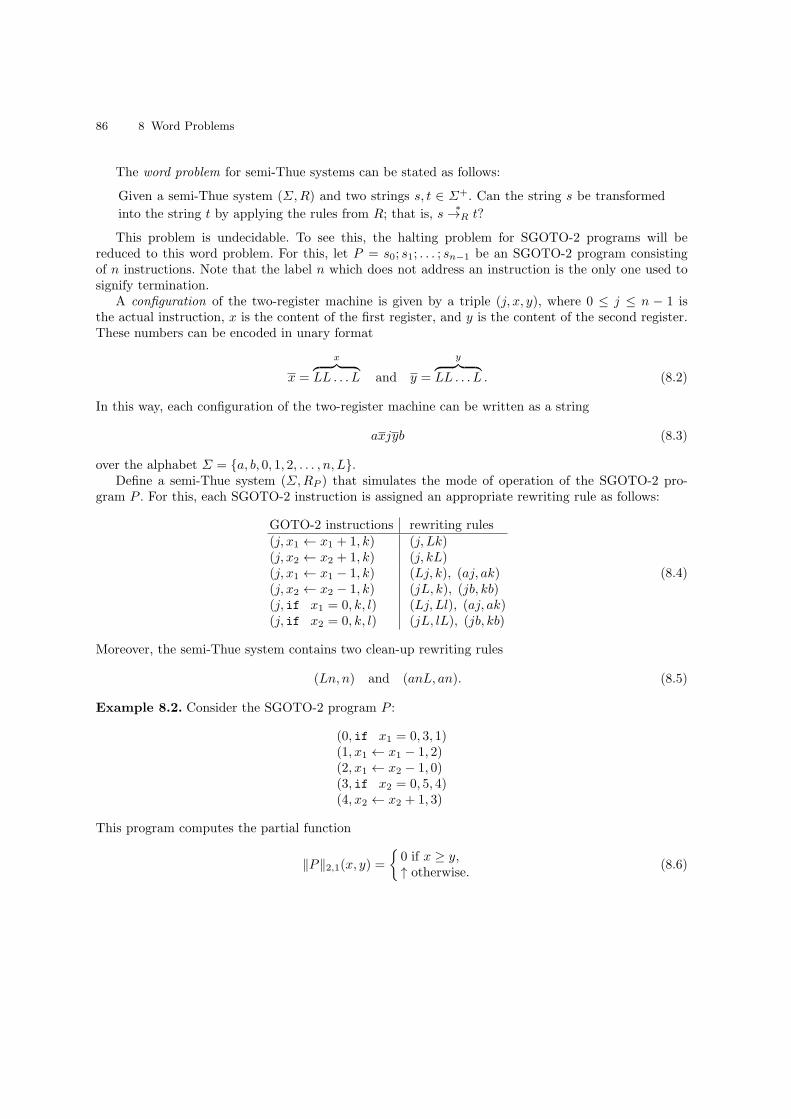
86 8 Word Problems
The word problem for semi-Thue systems can be stated as follows:
Given a semi-Thue system (Σ,R) and two strings s, t ∈ Σ+. Can the string s be transformed
into the string t by applying the rules from R; that is, s∗→R t?
This problem is undecidable. To see this, the halting problem for SGOTO-2 programs will bereduced to this word problem. For this, let P = s0; s1; . . . ; sn−1 be an SGOTO-2 program consistingof n instructions. Note that the label n which does not address an instruction is the only one used tosignify termination.
A configuration of the two-register machine is given by a triple (j, x, y), where 0 ≤ j ≤ n − 1 isthe actual instruction, x is the content of the first register, and y is the content of the second register.These numbers can be encoded in unary format
x =
x︷ ︸︸ ︷
LL . . . L and y =
y︷ ︸︸ ︷
LL . . . L . (8.2)
In this way, each configuration of the two-register machine can be written as a string
axjyb (8.3)
over the alphabet Σ = a, b, 0, 1, 2, . . . , n, L.Define a semi-Thue system (Σ,RP ) that simulates the mode of operation of the SGOTO-2 pro-
gram P . For this, each SGOTO-2 instruction is assigned an appropriate rewriting rule as follows:
GOTO-2 instructions rewriting rules(j, x1 ← x1 + 1, k) (j, Lk)(j, x2 ← x2 + 1, k) (j, kL)(j, x1 ← x1 − 1, k) (Lj, k), (aj, ak)(j, x2 ← x2 − 1, k) (jL, k), (jb, kb)(j, if x1 = 0, k, l) (Lj, Ll), (aj, ak)(j, if x2 = 0, k, l) (jL, lL), (jb, kb)
(8.4)
Moreover, the semi-Thue system contains two clean-up rewriting rules
(Ln, n) and (anL, an). (8.5)
Example 8.2. Consider the SGOTO-2 program P :
(0, if x1 = 0, 3, 1)(1, x1 ← x1 − 1, 2)(2, x1 ← x2 − 1, 0)(3, if x2 = 0, 5, 4)(4, x2 ← x2 + 1, 3)
This program computes the partial function
‖P‖2,1(x, y) =
0 if x ≥ y,↑ otherwise.
(8.6)
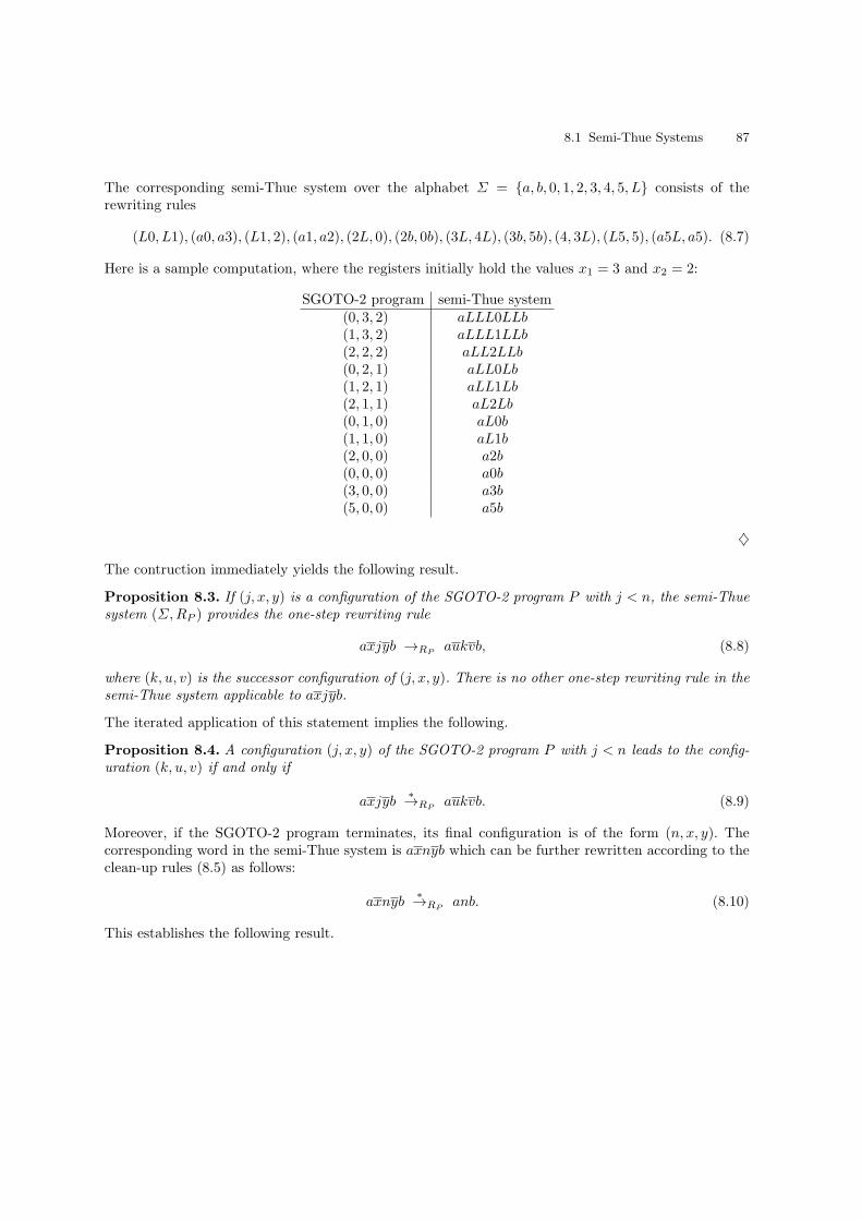
8.1 Semi-Thue Systems 87
The corresponding semi-Thue system over the alphabet Σ = a, b, 0, 1, 2, 3, 4, 5, L consists of therewriting rules
(L0, L1), (a0, a3), (L1, 2), (a1, a2), (2L, 0), (2b, 0b), (3L, 4L), (3b, 5b), (4, 3L), (L5, 5), (a5L, a5). (8.7)
Here is a sample computation, where the registers initially hold the values x1 = 3 and x2 = 2:
SGOTO-2 program semi-Thue system(0, 3, 2) aLLL0LLb(1, 3, 2) aLLL1LLb(2, 2, 2) aLL2LLb(0, 2, 1) aLL0Lb(1, 2, 1) aLL1Lb(2, 1, 1) aL2Lb(0, 1, 0) aL0b(1, 1, 0) aL1b(2, 0, 0) a2b(0, 0, 0) a0b(3, 0, 0) a3b(5, 0, 0) a5b
♦
The contruction immediately yields the following result.
Proposition 8.3. If (j, x, y) is a configuration of the SGOTO-2 program P with j < n, the semi-Thuesystem (Σ,RP ) provides the one-step rewriting rule
axjyb →RPaukvb, (8.8)
where (k, u, v) is the successor configuration of (j, x, y). There is no other one-step rewriting rule in thesemi-Thue system applicable to axjyb.
The iterated application of this statement implies the following.
Proposition 8.4. A configuration (j, x, y) of the SGOTO-2 program P with j < n leads to the config-uration (k, u, v) if and only if
axjyb∗→RP
aukvb. (8.9)
Moreover, if the SGOTO-2 program terminates, its final configuration is of the form (n, x, y). Thecorresponding word in the semi-Thue system is axnyb which can be further rewritten according to theclean-up rules (8.5) as follows:
axnyb∗→RP
anb. (8.10)
This establishes the following result.
88 8 Word Problems
Proposition 8.5. An SGOTO-2 program P started in the configuration (0, x, y) halts if and only if inthe corresponding semi-Thue system,
ax0yb∗→RP
anb. (8.11)
This proposition yields an effective reduction of the halting problem for SGOTO-2 programs to theword problem for semi-Thue systems. But the halting problem for SGOTO-2 programs is undecidableand thus we have established the following.
Theorem 8.6. The word problem for semi-Thue systems is undecidable.
8.2 Thue Systems
The Thue systems form a subclass of semi-Thue systems. A Thue system is a semi-Thue system (Σ,R)whose relation R is symmetric, i.e., if u → v ∈ R then v → u ∈ R. In a Thue system, the reflexivetransitive closure
∗→R of the one-step rewriting relation →R is also symmetric and thus an equivalence
relation on Σ+.The word problem can be summarized as follows:
Given a Thue system (Σ,R) and two strings s, t ∈ Σ+. Can the string s be transformed into
the string t by applying the rules from R; that is, s∗→R t?
This problem is also undecidable. To see this, Thue systems will be related to semi-Thue systems.For this, let (Σ,R) be a semi-Thue system. The symmetric closure of the rewriting relation R is thesymmetric relation
R(s) = R ∪R−1, (8.12)
where R−1 = (v, u) | (u, v) ∈ R is the inverse relation of R. The set R(s) is the smallest symmetric
relation containing R, and the pair (Σ,R(s)) is a Thue system. The relation∗→R(s) is thus the reflexive
transitive and symmetric closure of →R and hence an equivalence relation on Σ+. That is, for anystrings s, t ∈ Σ+, s
∗→R(s) t if and only if s = t or there is a finite sequence s0, s1, . . . , sm of elements in
Σ+ such that s = s0, si →R si+1 or si+1 →R si for 0 ≤ i ≤ m− 1, and sm = t. Note that if s∗→R(s) t
holds in a Thue system (Σ,R(s)), neither s∗→R t nor t
∗→R s need to be valid in the corresponding
semi-Thue system (Σ,R).
Example 8.7. Consider the semi-Thue system (Σ,R) with Σ = a, b and R = (ab, b), (ba, a). Thecorresponding Thue system is (Σ,R(s)), where R(s) = R ∪ (b, ab), (a, ba).
In the semi-Thue system, rewriting is strictly antitone leading to smaller strings, i.e., if u∗→R v and
u 6= v, then |u| > |v|, e.g., aabb→R abb→R bb.On the other hand, in the Thue system, aabb →R(s) abb →R(s) abab, but in the semi-Thue system
neither aabb∗→R abab nor abab
∗→R aabb. ♦
Theorem 8.8. (Post’s Lemma) Let P be an SGOTO-2 program with n instructions, let (Σ,RP )
be the corresponding semi-Thue system, and let (Σ,R(s)P ) be the associated Thue system. For each
configuration (j, x, y) of the program P ,
axjyb∗→RP
anb ⇐⇒ axjyb∗→R
(s)
P
anb. (8.13)

8.3 Semigroups 89
Proof. The direction from left-to-right holds since R ⊆ R(s). Conversely, let (j, x, y) be a configurationof the program P . By hypothesis, there is a rewriting sequence in the Thue system such that
s0 = axjyb→R
(s)
P
s1 →R(s)
P
. . .→R
(s)
P
sq = anb, (8.14)
where it may be assumed that the length q+1 of the derivation is minimal. It is clear that each occurringstring si corresponds to a configuration of the program P , 0 ≤ i ≤ q.
Suppose the derivation (8.14) cannot be established by the semi-Thue system. That is, the sequencecontains a rewriting step sp ←RP
sp+1, 0 ≤ p ≤ q − 1. The index p can be chosen to be maximal withthis property. Since there is no rewriting rule applicable to sq = anb, we have p+ 1 < q. This leads tothe following situation:
sp ←RPsp+1 →RP
sp+2. (8.15)
However, the string sp+1 encodes a configuration of P and there is at most one rewriting rule applicableto it. Thus the words sp and sp+2 must be identical and hence the derivation (8.14) can be shortenedby deleting the string sp+1 contradicting the assumption. ⊓⊔
The above result due to the Jewish logician Emil Post (1897-1954) provides an effective reductionof the derivations in semi-Thue system to derivations in Thue systems. But the word problem forsemi-Thue systems is undecidable and thus we obtain the following.
Theorem 8.9. The word problem for Thue systems is undecidable.
8.3 Semigroups
Word problems are also encountered in abstract algebra. A semigroup is an algebraic structure consistingof a non-empty set S together with an associative dyadic operation. For instance, the set of all non-empty strings Σ+ over an alphabet Σ together with the concatenation of strings is a semigroup, calledfree semigroup over Σ.
Each Thue system gives rise to a semigroup in a natural way. To see this, let (Σ,R(s)) be a Thue
system. We already know that the rewriting relation∗→R(s) on Σ+ is an equivalence relation. The
equivalence class of a string s ∈ Σ+ is the subset [s] of all strings in Σ+ that can be derived from s bya finite number of rewriting steps:
[s] = t ∈ Σ+ | s∗→R(s) t. (8.16)
Proposition 8.10. The set of equivalence classes H = H(Σ,R(s)) = [s] | s ∈ Σ+ forms a semigroupwith the operation
[s] [t] = [st], s, t ∈ Σ+. (8.17)
Proof. Claim that the operation is well-defined. Indeed, let [s] = [s′] and [t] = [t′], where s, s′, t, t′ ∈ Σ+.
Then s∗→R(s) s′, s′
∗→R(s) s, t
∗→R(s) t′, and t′
∗→R(s) t. Thus st
∗→R(s) s′t
∗→R(s) s′t′ and s′t′
∗→R(s)
st′∗→R(s) st. Hence, [st] = [s′t′]. ⊓⊔
90 8 Word Problems
The semigroup H = H(Σ,R(s)) can be defined by generators and relations. To see this, let Σ =a1, . . . , an and R = (u1, v1), . . . , (um, vm). Then the semigroup H has a presentation in terms ofgenerators and relations as follows:
H = 〈[a1], . . . , [an] | [u1] = [v1], . . . , [um] = [vm]〉.
The semigroup H is presented as the quotient of the free semigroup Σ+ by the subsemigroup of Σ+
generated by the relations [ui] = [vi], 1 ≤ i ≤ m.
Example 8.11. Consider the Thue system (Σ,R(s)), where Σ = a, b and R = (ab, b), (ba, a). Forinstance, a →R(s) ba →R(s) aba →R(s) aa and b →R(s) ab →R(s) bab →R(s) bb and thus [a] = [aa] and[b] = [bb]. The semigroup H = H(Σ,R(s)) has the presentation
H = 〈[a], [b] | [b] = [ab], [a] = [ba]〉.
Any word of H is of the form [ai1bj1 . . . aikbjk ], where i1, . . . , ik, j1, . . . , jk ≥ 0 with at least one ofthese numbers > 0. But the relations [b] = [ab] and [a] = [ba] imply [a] = [ba] = [aba] = [aa] and[b] = [ab] = [bab] = [bb]. Thus the semigroup H only consists of two elements [a] and [b] which areidempotent, i.e., [a] [a] = [a] and [b] [b] = [b], and satisfy [a] [b] = [b] and [b] [a] = [a]. ♦
The word problem for the semigroup H = H(Σ,R(s)) asks whether arbitrary strings s, t ∈ Σ+
describe the same element [s] = [t] or not. By definition,
[s] = [t] ⇐⇒ s∗→R(s) t, s, t ∈ Σ+. (8.18)
This equivalence provides an effective reduction of the word problem for Thue systems to the wordproblem for semigroups. This leads to the following result which was independently established byEmil Post (1987-1954) and Andrey Markov Jr. (1903-1979).
Theorem 8.12. The word problem for semigroups is undecidable.
8.4 Post’s Correspondence Problem
The Post correspondence problem is an undecidable problem that was introduced by Emil Post in 1946.Due to its simplicity it is often used in proofs of undecidability.
A Post correspondence system (PCS) over an alphabet Σ is a finite setΠ of pairs (αi, βi) ∈ Σ+×Σ+,
1 ≤ i ≤ m. For each finite sequence i = (i1, . . . , ir) ∈ 1, . . . ,m+ of indices, define the strings
α(i) = αi1 αi2 · · · αir (8.19)
and
β(i) = βi1 βi2 · · · βir . (8.20)
A solution of the PCS Π is a sequence i of indices such that α(i) = β(i).
8.4 Post’s Correspondence Problem 91
Example 8.13. The PCS Π = (α1, β1) = (a, aaa), (α2, β2) = (abaa, ab), (α3, β3) = (aab, b) over thealphabet Σ = a, b has the solution i = (2, 1, 1, 3), since
α(i) = α2 α1 α1 α3 = abaa a a aab
= abaaaaaab
= ab aaa aaa b = β2 β1 β1 β3 = β(i).
♦
The word problem for Post correspondence systems asks whether a Post correspondence system hasa solution or not. This problem is undecidable. To see this, the word problem for semi-Thue systemswill be reduced to this one. To this end, let (Σ,R) be a semi-Thue system, where Σ = a1, . . . , anand R = (ui, vi) | 1 ≤ i ≤ m. Take a copy of the alphabet Σ given by Σ′ = a′1, . . . , a
′n. In this way,
each string s = ai1ai2 . . . air over Σ can be assigned a copy s′ = a′i1a′i2. . . a′ir over Σ′.
Put q = m+n and let s, t ∈ Σ+. Define the PCSΠ = Π(Σ,R, s, t) over the alphabetΣ∪Σ′∪x, y, zby the following 2q + 4 pairs:
(αi, βi) = (ui, v′i), 1 ≤ i ≤ m,
(αm+i, βm+i) = (ai, a′i), 1 ≤ i ≤ n,
(αq+i, βp+i) = (u′i, vi), 1 ≤ i ≤ m,
(αq+m+i, βp+m+i) = (a′i, ai), 1 ≤ i ≤ n, (8.21)
(α2q+1, β2p+1) = (y, z),
(α2q+2, β2p+2) = (z, y),
(α2p+3, β2p+3) = (x, xsy),
(α2p+4, β2p+4) = (ztx, x).
Example 8.14. Take the semi-Thue system (Σ,R), whereΣ = a, b andR = (ab, bb), (ab, a), (b, aba).The corresponding PCS Π = Π(Σ,R, s, t) over the alphabet a, b, a′, b′, x, y, z consists of the followingpairs:
(ab, b′b′),(ab, a′),(b, a′b′a′),(a, a′),(b, b′),(a′b′, bb),(a′b′, a),(b′, aba),(a′, a),(b′, b),(y, z),(z, y),(x, xsy),(ztx, x).
♦
92 8 Word Problems
First, observe that the derivations of a semi-Thue system can be mimicked by the correspondingPCS.
Proposition 8.15.
• If s, t ∈ Σ+ with s = t or s→R t, there is a sequence i ∈ 1, . . . , q+ of indices such that α(i) = sand β(i) = t′, and there is a sequence i′ ∈ q + 1, . . . , 2q+ of indices such that α(i′) = s′ andβ(i′) = t.
• If s, t ∈ Σ+ such that there is a sequence i ∈ 1, . . . , q+ of indices such that α(i) = s and β(i) = t′,
then s∗→R t.
• If s, t ∈ Σ+ such that there is a sequence i′ ∈ q + 1, . . . , 2q+ of indices such that α(i′) = s′ and
β(i′) = t, then s∗→R t.
Example 8.16. (Cont’d) Let s = aabb and t = aab. Then s →R t by the rule (ab, a) ∈ R and thesequences i = (4, 2, 5) and i′ = (9, 7, 10) yield
α(i) = α4 α2 α5 = a ab b = aabb,
β(i) = β4 β2 β5 = a′ a′ b′ = a′a′b′,
α(i′) = α9 α7 α10 = a′ a′b′ b′ = a′a′b′b′,
β(i′) = β9 β7 β10 = a a b = aab.
Let s = bbaba = α(5, 3, 2, 4) and t′ = b′a′b′a′a′a′ = β(5, 3, 2, 4). Then s = bbaba →R babaaba →R
babaaa = t and so s∗→R t. ♦
Second, the solutions of the constructed PCS can always be canonically decomposed.
Proposition 8.17.
• Let i = (i1, . . . , ir) be a solution of the PCS Π = Π(Σ,R, s, t) with w = α(i) = β(i). If w = w1yw2
for some w1, w2 ∈ Σ′∗, there is an index j, 1 ≤ j ≤ r, such that
α(i1, . . . , ij−1) = w1, α(ij) = y, and α(ij+1, . . . , ir) = w2. (8.22)
• Let i = (i1, . . . , ir) be a solution of the PCS Π = Π(Σ,R, s, t) with w = α(i) = β(i). If w = w1zw2
for some w1, w2 ∈ Σ′∗, there is an index j, 1 ≤ j ≤ r, such that either
α(i1, . . . , ij−1) = w1, α(ij) = z, and α(ij+1, . . . , ir) = w2, (8.23)
or
α(i1, . . . , ij−1) = w1, α(ij) = ztx, α(ij+1, . . . , ir) = u, and w2 = txu. (8.24)
Example 8.18. (Cont’d) Let s = b and t = abaa. A solution of the PCS Π is given by
i = (13, 3, 11, 6, 9, 12, 3, 5, 4, 11, 9, 10, 7, 9, 14),
since
8.4 Post’s Correspondence Problem 93
α(i) = x b y a′b′ a′ z b b a y a′ b′ a′b′ a′ zabaax
= xbya′b′a′zbbaya′b′a′b′a′zabaax
= xby a′b′a′ z bb a y a′b′a′ b′ a′ z a b a a x
= β(i).
Here we have
w1 = xbya′b′a′zbba = α(13, 3, 11, 6, 9, 12, 3, 5, 4)
and
w2 = a′b′a′b′a′zabaax = α(9, 10, 7, 9, 14),
or
w1 = xbya′b′a′ = α(13, 3, 11, 6, 9)
and
w2 = bbaya′b′a′b′a′zabaax = α(3, 5, 4, 11, 9, 10, 7, 9, 14),
or
w1 = xbya′b′a′zbbaya′b′a′b′a′ = α(13, 3, 11, 6, 9, 3, 5, 4, 11, 9, 10, 7, 9),
and
ztx = zabaax = α(14) and w2 = abaax = tx.
♦
Note that if the PCS Π = Π(Σ,R, s, t) has a solution α(i) = β(i) with i = (i1, . . . , ir), the solutionstarts with i1 = 2q + 3 and ends with ir = 2p+ 4, i.e., the corresponding string has the prefix xsy andthe postfix ztx. The reason is that (α2p+3, β2p+3) = (x, xsy) is the only pair whose components havethe same prefix and (α2p+4, β2p+4) = (ztx, x) is the only pair whose components have the same postfix.
Proposition 8.19. Let s, t ∈ Σ+. If there is a derivation s∗→R t in the semi-Thue system (Σ,R), the
PCS Π = Π(Σ,R, s, t) has a solution.
Proof. Let s∗→R t with
s = s1 →R s2 →R . . .→R sk−1 →R sk = t, (8.25)
where si →R si+1 or si = si+1, 0 ≤ i ≤ k − 1. The inclusion of steps without effect allows to assume
that k is odd. By Proposition 8.15, for each j, 1 ≤ j < k, there is a sequence i(j) of indices such thatα(i(j)) = sj and β(i
(j)) = s′j+1 if j is odd and α(i(j)) = s′j and β(i(j)) = sj+1 if j is even.
Claim that a solution of the PCS is given by the sequence
94 8 Word Problems
i = (2p+ 3, i(1), 2p+ 1, i(2), 2p+ 2, i(3), 2p+ 1, . . . , i(k−2), 2p+ 1, i(k−1), 2p+ 4). (8.26)
Indeed, the sequence can be evaluated as follows:
α(i) : x s1 y s′2 z s3 y . . . sk−2 y s′k−1 zskx. . . . . . . . . . .
i : 2p+ 3 i(1) 2p+ 1 i(2) 2p+ 2 i(3) 2p+ 1 . . . i(k−2) 2p+ 1 i(k−1) 2p+ 4. . . . . . . . . . .
β(i) : xs1y s′2 z s3 y s′4 z . . . s′k−1 z sk x
This proves the claim. ⊓⊔
Example 8.20. (Cont’d) Consider the derivation
s = aab→R abb→ abb→R aabab→R aaab→R aaa = t.
A solution of the PCS Π = Π(Σ,R, aab, aaa) is given by the sequence
i = (13, 4, 1, 11, 9, 8, 10, 12, 4, 2, 4, 5, 11, 9, 9, 7, 14),
whereα(i) : x aab y a′b′b′ z aabab y a′a′a′b′ zaaax
. . . . . . . . .i : 13 (4, 1) 11 (9, 8, 10) 12 (4, 2, 4, 5) 11 (9, 9, 7) 14
. . . . . . . . .β(i) : xaaby a′b′b′ z aabab y a′a′a′b′ z aaa x
♦
Proposition 8.21. Let s, t ∈ Σ+. If the PCS Π = Π(Σ,R, s, t) has a solution, there is a derivation
s∗→R t in the semi-Thue system (Σ,R).
Proof. Let i = (i1, . . . , ir) be a minimal solution of the PCSΠ. The observation prior to Proposition 8.19shows that the string w = α(i) = β(i) must have the form w = xsy . . . ztx.
By Proposition 8.17, there is a sequence i(1) of indices such that α(i(1)) = s = s1. Put s′2 = β(i(1)).
It follows that w = xs1ys′2z . . . and by Proposition 8.15, s1
∗→R s2.
By Proposition 8.17, there is a sequence i(2) of indices such that α(i(2)) = s′2. Set s3 = β(i(2)). Thus
w = xs1ys′2zs3 . . . and by Proposition 8.15, s2
∗→R s3.
By Proposition 8.17, there are two possibilities:
• Let i = (2q + 3, i(1), 2q + 1, i(2), 2q + 2, . . .), i.e., w = xs1ys′2zs3y . . .. Then the sequence can be
continued as indicated above.• Let i = (2q + 3, i(1), 2q + 1, i(2), 2q + 4, . . .). This is only possible if s3 = t and w = xs1ys
′2ztx. It
follows that i = (2q + 3, i(1), 2q + 1, i(2), 2q + 4) is already a solution due to minimality:
α(i) : x s1 y s′2 ztx. . . . .
i : 2q + 3 i(1) 2q + 1 i(2) 2q + 4. . . . .
β(i) : xs1y s′2 z t x
But s = s1∗→R s2 and s2
∗→R s3 = t, and so s
∗→R t.
8.4 Post’s Correspondence Problem 95
By induction, there are strings s = s1, s2, s3, . . . , sk = t in Σ+ with k odd such that
α(i) = x s1 y s′2 z s3 . . . sk−2 y s
′k−1 z sk x = β(i)
and si∗→R si+1, 1 ≤ i ≤ k − 1. Hence, s
∗→R t as required. ⊓⊔
Example 8.22. (Cont’d) Let s = b and t = abaa. A solution of the PCS Π is given by
i = (13, 3, 11, 6, 9, 12, 3, 5, 4, 11, 9, 10, 7, 9, 14).
The string
α(i) = β(i) = xbya′b′a′zbbaya′b′a′b′a′zabaax
provides a derivation in the semi-Thue system:
s = b∗→R aba
∗→R bba
∗→R ababa
∗→R abaa = t.
♦
The last two propositions provide a reduction of the word problem for semi-Thue systems to the wordproblem for Post correspondence systems. But the word problem for semi-Thue systems is undecidable.This gives rise to the following result.
Theorem 8.23. The word problem for Post correspondence systems is undecidable.

Index
abstract rewriting system, 85acceptable programming system, 57Ackermann, Wilhelm, 39anti-diagonal, 19asymmetric difference, 2
basic function, 11bifurcation label, 31blank, 59block, 4bounded minimalization, 17bounded product, 17bounded quantification
existential, 22universal, 22
bounded sum, 17
Cantor function, 19Cantor, Georg, 70characteristic function, 22Church, Alonso, 38composition, 2, 11, 14computable function, 5configuration, 32, 66, 86constant function
0-ary, 111-ary, 11
copy, 7cosign function, 17
Davis, Martin, 61decidable set, 69decision procedure, 69
partial, 74
decrement function, 2Dedekind, Richard, 10depth, 24derivation, 85diagonalization, 70diophantine equation, 80
linear, 80diophantine set, 81domain, 2
empty string, 49enumerator, 77equivalence class, 89Euler, Leonhard, 81extension, 78
functiondefined by cases, 16finite, 78GOTO computable, 34LOOP computable, 24partial, 2partial recursive, 30Post-Turing computable, 66recursive, 30total, 2URM computable, 5
Fundamental Lemma, 10
Godel number, 49instruction, 52program, 52
Godel numbering, 49, 66Godel, Kurt, 49
98 Index
GOTO computability, 34GOTO program, 31
instruction, 31standard, 31, 51termination, 32
graph, 2, 76
halt state, 59halting problem, 71Hilbert, David, 80
increment function, 2index, 52, 77induction axiom, 9input alphabet, 59inverse relation, 88iteration, 3, 21
Kleene predicate, 58Kleene set, 57Kleene, Stephen Cole, 29, 53
label, 31Lagrange, Joseph-Louis, 81left move, 59length function, 51LOOP
complexity, 43computability, 24program, 24
Markov, Andrey, 90Matiyasevich, Yuri, 81morphism, 9
natural variety, 80next label, 31non-move, 59normal form, 58
one-step function, 32, 54iterated, 56
pairing function, 19parametrization, 16partial function, 2partial recursive function, 30PCS, 90
solution, 90Peano structure, 9
semi, 9Peano, Guiseppe, 9Post correspondence system
see PCS, 90Post, Emil, 89, 90Post-Turing
machine, 61program, 61
power, 3, 21presentation, 90primitive recursion, 11, 12primitive set, 22primitively closed, 14projection function, 11
r.e., 76range, 2rational numbers, 70recursive enumerable set, 76recursive function, 30recursive set, 76reducibility, 71reduction, 70reduction function, 71reload, 7residual step function, 33, 57, 67rewriting rule, 85Rice theorem, 73Rice, Henry Gordon, 73Rice-Shapiro theorem, 79right move, 59runtime function, 33, 56, 67
semi-Thue system, 85semidecidable set, 73semigroup, 89
free, 89semigroup of transformations, 3SGOTO program, 51Shapiro, Norman, 78smn theorem, 53start state, 59state transition function, 59string rewriting system, 85successor configuration, 32successor function, 9, 11symmetric closure, 88
tape alphabet, 59
Index 99
thesis of Church, 38Thue system, 88Thue, Axel, 85total function, 2transformation of variables, 15translation invariance, 6Turing machine, 59
computation, 60configurationinitial, 60
state, 59Turing, Alan, 59, 71
unbounded minimalization, 29, 57existential, 57universal, 58
undecidable set, 69universal function, 54unlimited register machine
see URM, 1
URM, 1
computable function, 5
composition, 4
computability, 5
iteration, 4
program, 3
atomic, 4
normal, 6
state set, 1
URM program
semantics, 4
word problem
PCS, 91
semi-Thue system, 86
semigroup, 90
Thue system, 88

100 Index

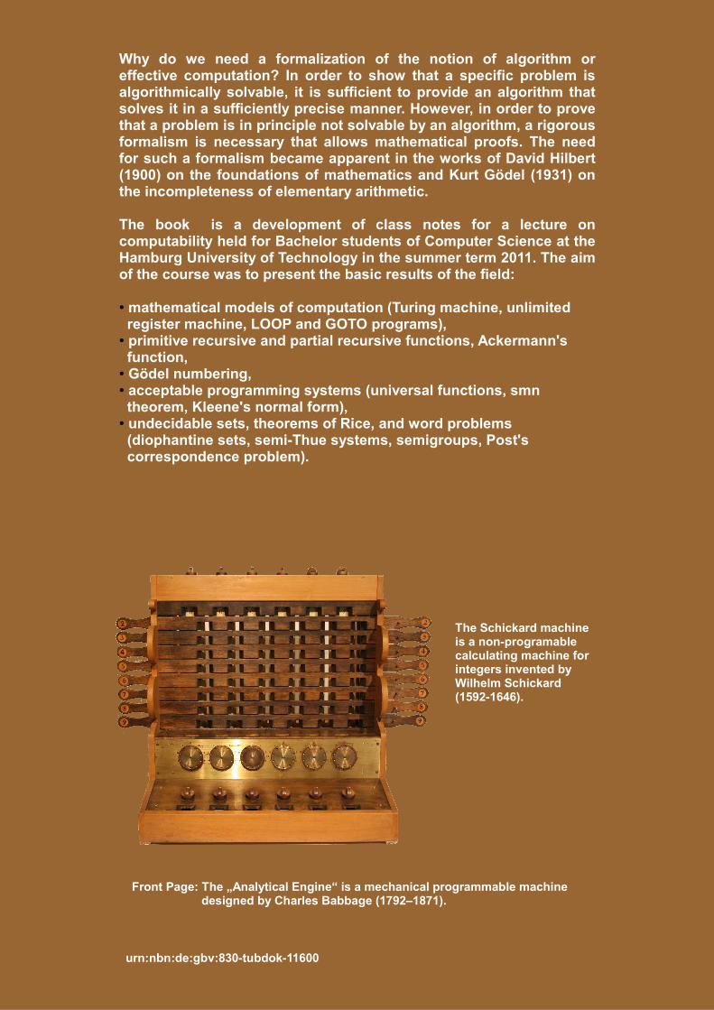
Why do we need a formalization of the notion of algorithm or effective computation? In order to show that a specific problem is algorithmically solvable, it is sufficient to provide an algorithm that solves it in a sufficiently precise manner. However, in order to prove that a problem is in principle not solvable by an algorithm, a rigorous formalism is necessary that allows mathematical proofs. The need for such a formalism became apparent in the works of David Hilbert (1900) on the foundations of mathematics and Kurt Gödel (1931) on the incompleteness of elementary arithmetic.
The book is a development of class notes for a lecture on computability held for Bachelor students of Computer Science at the Hamburg University of Technology in the summer term 2011. The aim of the course was to present the basic results of the field:
mathematical models of computation (Turing machine, unlimited register machine, LOOP and GOTO programs), primitive recursive and partial recursive functions, Ackermann's function, Gödel numbering, acceptable programming systems (universal functions, smn theorem, Kleene's normal form), undecidable sets, theorems of Rice, and word problems (diophantine sets, semi-Thue systems, semigroups, Post's correspondence problem).
The Schickard machine is a non-programable calculating machine for integers invented by Wilhelm Schickard (1592-1646).
Front Page: The „Analytical Engine“ is a mechanical programmable machine designed by Charles Babbage (1792–1871).
urn:nbn:de:gbv:830-tubdok-11600


![Local function vs. local closure function · Local function vs. local closure function ... Let ˝be a topology on X. Then Cl (A) ... [Kuratowski 1933]. Local closure function](https://static.fdocument.org/doc/165x107/5afec8997f8b9a256b8d8ccd/local-function-vs-local-closure-function-vs-local-closure-function-let-be.jpg)