![Cadenas de Markov - cimat.mxjortega/MaterialDidactico/probabilidad17/Tema4.pdf · Como en el ejemplo anterior 2[0;1] denota la probabilidad de que llegue una llamada y 2[0;1] la probabilidad](https://static.fdocument.org/doc/165x107/5e233278f307ec29123fe1ac/cadenas-de-markov-cimatmx-jortegamaterialdidacticoprobabilidad17tema4pdf.jpg)
Colorado State University - math.colostate.eduwangz/m535 presentation/m535... · Numerical...
15
Poroelasticity Zhuoran Wang Colorado State University Zhuoran Wang Poroelasticity
Transcript of Colorado State University - math.colostate.eduwangz/m535 presentation/m535... · Numerical...

Poroelasticity
Zhuoran Wang
Colorado State University
Zhuoran Wang Poroelasticity
Linear poroelasticity
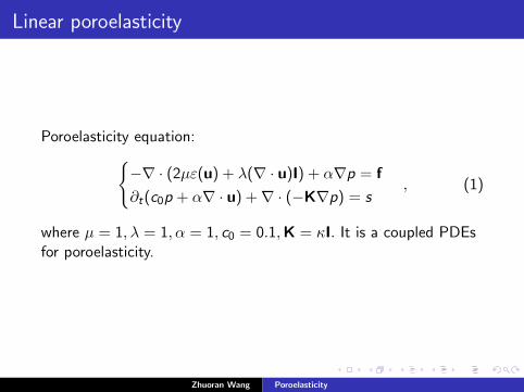
Poroelasticity equation:−∇ · (2µε(u) + λ(∇ · u)I) + α∇p = f
∂t(c0p + α∇ · u) +∇ · (−K∇p) = s, (1)
where µ = 1, λ = 1, α = 1, c0 = 0.1,K = κI. It is a coupled PDEsfor poroelasticity.
Zhuoran Wang Poroelasticity
Numerical experiments for linear poroelasticity
We test the example which is on (0, 1)2 for linear poroelasicity.Dirichlet boundary condition for displacement is uD = u and forpressure is pD = p.
Zhuoran Wang Poroelasticity
Numerical experiments for linear poroelasticity
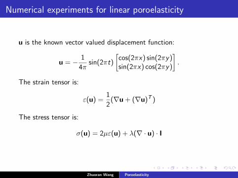
u is the known vector valued displacement function:
u = − 1
4πsin(2πt)
[cos(2πx) sin(2πy)sin(2πx) cos(2πy)
].
The strain tensor is:
ε(u) =1
2(∇u + (∇u)T )
The stress tensor is:
σ(u) = 2µε(u) + λ(∇ · u) · I
Zhuoran Wang Poroelasticity
Numerical experiments for linear poroelasticity
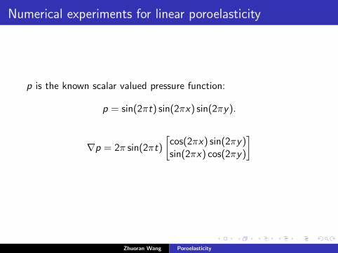
p is the known scalar valued pressure function:
p = sin(2πt) sin(2πx) sin(2πy).
∇p = 2π sin(2πt)
[cos(2πx) sin(2πy)sin(2πx) cos(2πy)
]
Zhuoran Wang Poroelasticity
Numerical experiments for linear poroelasticity
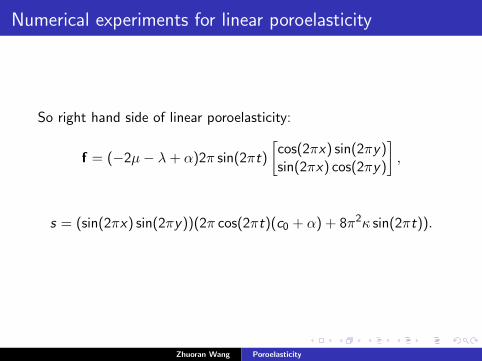
So right hand side of linear poroelasticity:
f = (−2µ− λ+ α)2π sin(2πt)
[cos(2πx) sin(2πy)sin(2πx) cos(2πy)
],
s = (sin(2πx) sin(2πy))(2π cos(2πt)(c0 + α) + 8π2κ sin(2πt)).
Zhuoran Wang Poroelasticity
Numer. Exp.: Rectangular Meshes:Profiles of numerical displacement & pressure
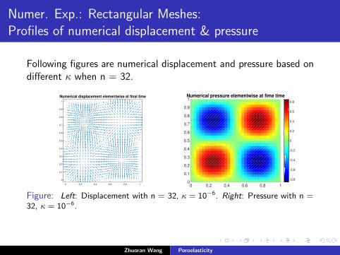
Following figures are numerical displacement and pressure based ondifferent κ when n = 32.
0 0.2 0.4 0.6 0.8 1
0
0.1
0.2
0.3
0.4
0.5
0.6
0.7
0.8
0.9
1
Numerical displacement elementwise at final time
0 0.2 0.4 0.6 0.8 10
0.1
0.2
0.3
0.4
0.5
0.6
0.7
0.8
0.9
1Numerical pressure elementwise at fime time
-0.8
-0.6
-0.4
-0.2
0
0.2
0.4
0.6
0.8
Figure: Left: Displacement with n = 32, κ = 10−6. Right: Pressure with n =32, κ = 10−6.
Zhuoran Wang Poroelasticity

Numer. Exp.: Rectangular Meshes:Profiles of numerical displacement & pressure
0 0.1 0.2 0.3 0.4 0.5 0.6 0.7 0.8 0.9 1
0
0.1
0.2
0.3
0.4
0.5
0.6
0.7
0.8
0.9
1
Numerical displacement elementwise at final time
0 0.2 0.4 0.6 0.8 10
0.1
0.2
0.3
0.4
0.5
0.6
0.7
0.8
0.9
1Numerical pressure elementwise at fime time
-0.8
-0.6
-0.4
-0.2
0
0.2
0.4
0.6
0.8
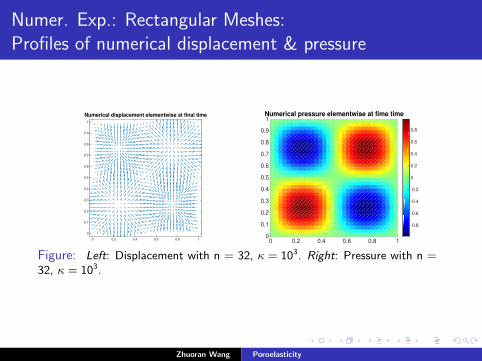
Figure: Left: Displacement with n = 32, κ = 1. Right: Pressure with n = 32,κ = 1.
Zhuoran Wang Poroelasticity
Numer. Exp.: Rectangular Meshes:Profiles of numerical displacement & pressure
0 0.2 0.4 0.6 0.8 1
0
0.1
0.2
0.3
0.4
0.5
0.6
0.7
0.8
0.9
1
Numerical displacement elementwise at final time
0 0.2 0.4 0.6 0.8 10
0.1
0.2
0.3
0.4
0.5
0.6
0.7
0.8
0.9
1Numerical pressure elementwise at fime time
-0.8
-0.6
-0.4
-0.2
0
0.2
0.4
0.6
0.8
Figure: Left: Displacement with n = 32, κ = 103. Right: Pressure with n =32, κ = 103.
Zhuoran Wang Poroelasticity
Numer. Exp.: Rectangular Meshes:Profiles of numerical displacement & pressure
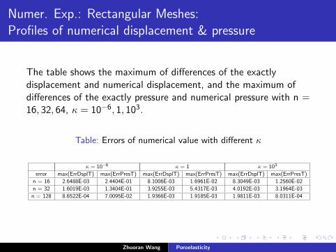
The table shows the maximum of differences of the exactlydisplacement and numerical displacement, and the maximum ofdifferences of the exactly pressure and numerical pressure with n =16, 32, 64, κ = 10−6, 1, 103.
Table: Errors of numerical value with different κ
κ = 10−6 κ = 1 κ = 103
error max(ErrDsplT) max(ErrPresT) max(ErrDsplT) max(ErrPresT) max(ErrDsplT) max(ErrPresT)
n = 16 2.6488E-03 2.4404E-01 8.1006E-03 1.6961E-02 8.3049E-03 1.2560E-02
n = 32 1.6019E-03 1.3404E-01 3.9255E-03 5.4317E-03 4.0192E-03 3.1964E-03
n = 128 8.6522E-04 7.0095E-02 1.9366E-03 1.9185E-03 1.9811E-03 8.0311E-04
Zhuoran Wang Poroelasticity
Numer. Exp.: Rectangular Meshes:Profiles of numerical displacement & pressure
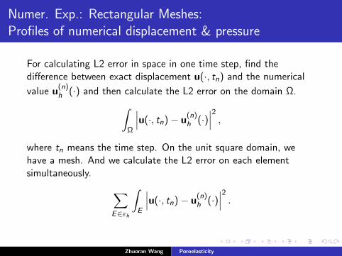
For calculating L2 error in space in one time step, find thedifference between exact displacement u(·, tn) and the numerical
value u(n)h (·) and then calculate the L2 error on the domain Ω.∫
Ω
∣∣∣u(·, tn)− u(n)h (·)
∣∣∣2 ,where tn means the time step. On the unit square domain, wehave a mesh. And we calculate the L2 error on each elementsimultaneously. ∑
E∈εh
∫E
∣∣∣u(·, tn)− u(n)h (·)
∣∣∣2 .
Zhuoran Wang Poroelasticity
Numer. Exp.: Rectangular Meshes:Profiles of numerical displacement & pressure
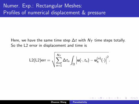
Here, we have the same time step ∆t with NT time steps totally.So the L2 error in displacement and time is
L2(L2)err =
√√√√ NT∑n=1
∆tn
∫Ω
∣∣∣u(·, tn)− u(n)h (·)
∣∣∣2.
Zhuoran Wang Poroelasticity

Numer. Exp.: Rectangular Meshes:Profiles of numerical displacement & pressure
Table: Convergence rates of errors in the numerical displacement withtime steps,Q1.
n L2L2ErrDispl. conv. raten = 8 2.1187E-03 –n = 16 6.8777E-04 1.6232n = 32 2.6531E-04 1.3742n = 64 1.1697E-04 1.1815n = 128 5.5224E-05 1.0828
Zhuoran Wang Poroelasticity
Numer. Exp.: Rectangular Meshes:Profiles of numerical displacement & pressure
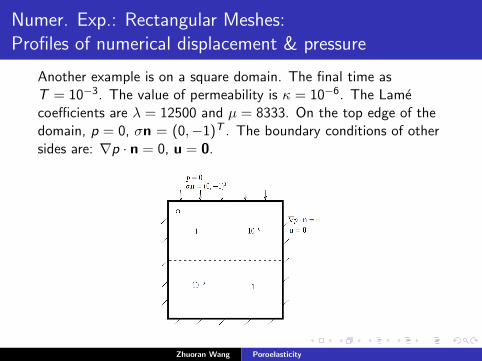
Another example is on a square domain. The final time asT = 10−3. The value of permeability is κ = 10−6. The Lamecoefficients are λ = 12500 and µ = 8333. On the top edge of thedomain, p = 0, σn = (0,−1)T . The boundary conditions of othersides are: ∇p · n = 0, u = 0.
Zhuoran Wang Poroelasticity
Numer. Exp.: Rectangular Meshes:Profiles of numerical displacement & pressure
0 0.2 0.4 0.6 0.8 10
0.1
0.2
0.3
0.4
0.5
0.6
0.7
0.8
0.9
1Numerical pressure elementwise at final time
0.1
0.2
0.3
0.4
0.5
0.6
0.7
0.8
0.9
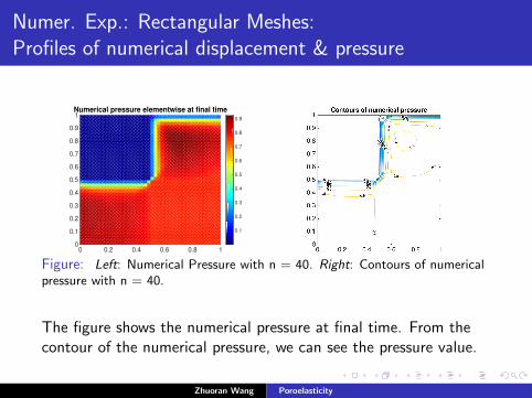
Figure: Left: Numerical Pressure with n = 40. Right: Contours of numericalpressure with n = 40.
The figure shows the numerical pressure at final time. From thecontour of the numerical pressure, we can see the pressure value.
Zhuoran Wang Poroelasticity