Color Constancy, Intrinsic Images, and Shape Estimation ......Jonathan T. Barron and Jitendra Malik...

Color Constancy, Intrinsic Images,and Shape Estimation (Supplementary Material)

Jonathan T. Barron and Jitendra Malik{barron, malik}@eecs.berkeley.edu

UC Berkeley

1 Priors on Shape

Our prior on shape f(Z) is very similar to that of [1]. It is a linear combinationof three costs:

f(Z) = λfff (Z) + λcfc(Z) + λkfk(Z) (1)

where ff (Z) is a “flatness” term that encourages shapes to be fronto-parallel,fc encourages shapes to face outward at the bounding contour, and fk is asmoothness term that penalizes variation in mean curvature. The λ multipliersare learned through cross-validation on the training set. Our ff (Z) and fc(Z)terms are identical to [1], but we present a refinement to fk(Z): we make themodel single-scale (as multiscale priors don’t improve performance significantlywith our new multiscale optimization technique), and instead of placing a penaltyon the gradient norm of mean curvature, we place the penalty on the pairwisevariation of mean curvature between all pixels in a small window, which improvesperformance. Formally, our prior is:

fk(Z) =∑i

∑j∈N(i)

log

(K∑k=1

αkN (H(Z)i −H(Z)j ; 0,σk)

)(2)

where N(i) is the 5×5 neighborhood around pixel i, H(Z) is the mean curvatureof shape Z, H(Z)i − H(Z)j is the difference between the mean curvature atpixel i and pixel j, K = 40 (the GSM has 40 discrete Gaussians), α are mixingcoefficients, σ are the standard deviations of the Gaussians in the mixture. Themean is set to 0, as the most likely shapes should have constant mean curvature(like planes, spheres, cylinders, soap bubbles, etc). The GSM is learned usingEM on the training set.

To review, mean curvature is defined as the average of principle curvatures:H = 1

2 (κ1 + κ2). It can be approximated using the first and second partialderivatives of a surface:

H(Z) =

(1 + Z2

x

)Zyy − 2ZxZyZxy +

(1 + Z2

y

)Zxx

2(1 + Z2

x + Z2y

)3/2See [1] for a thorough explanation of how this can be calculated and differentiatedefficiently with filter convolutions.

2 Jonathan T. Barron and Jitendra Malik

2 Global Reflectance Entropy

Renyi measures of entropy are quadratically expensive to compute naively, soothers have used the Fast Gauss Transform [2] and histogram-based techniques [1]to approximate them in linear time. We will generalize the algorithm of [1] forcomputing 1D entropy to our 3D case.

Given 3 × n matrix X = [x1,x2, · · · ,xn] we construct a 3D histogram Γ asfollows. Γ is initialized to 0, and then for each vector x we increment the eightsurrounding bins in Γ by fractions that sum to 1 using trilinear interpolation:

Γ(⌊x1

s

⌋,⌊x2s

⌋,⌊x3s

⌋)+=

(⌈x1s

⌉− x1

s

)(⌈x2s

⌉− x2

s

)(⌈x3s

⌉− x3

s

)Γ(⌊x1

s

⌋,⌊x2s

⌋,⌈x3s

⌉)+=

(⌈x1s

⌉− x1

s

)(⌈x2s

⌉− x2

s

)(x3s−⌊x3s

⌋)· · ·

Γ(⌈x1

s

⌉,⌈x2s

⌉,⌊x3s

⌋)+=

(x1s−⌊x1s

⌋)(x2s−⌊x2s

⌋)(⌈x3s

⌉− x3

s

)Γ(⌈x1

s

⌉,⌈x2s

⌉,⌈x3s

⌉)+=

(x1s−⌊x1s

⌋)(x2s−⌊x2s

⌋)(x3s−⌊x3s

⌋)Where s is a scale parameter that controls the bin-width of the histogram, andimplicitly, accuracy. Using interpolation makes our binning operation smoothand differentiable, which is necessary for calculating the analytic gradient of Hwith respect to X. With this histogram, we create a new blurred histogramΓ = G ∗ Γ, where G is a three-dimensional Gaussian kernel. This kernel isseparable, so we can instead convolve Γ with the a one-dimensional Gaussian

kernel g = N (0,√2σs ) in the three dimensions:

Γ = g1 ∗ (g2 ∗ (g3 ∗ Γ)) (3)

With this, the following is a good approximation to our entropy measure:

H(X, σ) ≈ − log

∑i,j,k

Γi,j,k × Γi,j,k

(4)

Which is just the negative log of the inner product between the two histograms.We omit the proof of correctness for brevity’s sake, but it looks very similar tothe proof of the 1D case in [1]. The analytical derivatives of H with respect toX can be calculated efficiently in the manner of [1].

Note that this formulation is extremely similar to the bilateral grid [3], whichis a tool for high-dimensional Gaussian filtering (used mostly for bilateral filter-ing, hence the name). The calculation of our entropy measure is extremely similarto the “splat, blur, slice” pipeline in other high-dimensional Gaussian filteringworks [4], except that after the “slice” operation we take the inner product ofthe input “signal” and the blurred output signal. This means that we need notactually compute the slice operation, but can instead just compute the innerproduct directly in the histogram space. This connection means that the body

Color Constancy, Intrinsic Images, and Shape Estimation (Supp.) 3

of work for efficiently computing this quantity in the context of image filteringcan be directly adapted to the problem of computing high-dimensional entropymeasures. Recent work [4] suggests that for dimensionalities of 3, our bilateralgrid formulation is the most efficient among existing techniques, but that thisentropy measure could be computed reasonably efficiently in significantly higher-dimensionality spaces (up to 8 or 16) using more sophisticated techniques.

3 Error Metrics

Choosing good error metrics is challenging. Our error metrics are a revision ofthose in our previous work [1]. We will use the geometric mean of five errormetrics: one for shape, one for illumination, one for shading, one for reflectance,and the MIT intrinsic images error metric introduced in [5], which we will referto as rs-MSE (though which the original authors call “LMSE”). We use thegeometric mean of these metrics as it is insensitive to the different dynamicranges of the constituent error metrics, and is difficult to trivially minimize inpractice.

Our shape error metric is:

N -MSE(N ,N∗) =1

n

∑x,y

arccos(Nx,y ·N∗x,y

)2(5)

This is the mean square error between the angle the normal field N of ourestimated shape Z and the normal field N∗ of the ground-truth shape Z∗, inradians. This error metric is invariant to shifts in Z, but is sensitive to othererrors.

For illumination, our error metric is:

L -MSE(L, L∗) =1

nminα

∑x,y

||αV (L)x,y − V (L∗)x,y||22 (6)

Which is the scale-invariant MSE of a rendering of our recovered illumination Land the ground-truth illumination L∗. V (L) is a function that renders the spher-ical harmonic illumination L on a sphere and returns the log-shading. V (L)x,yis a 3-vector of log-RGB at position (x, y) in the renderings. The α multipliermakes this error metric invariant to absolute scaling, meaning that estimatingillumination to be twice as bright or half as bright doesn’t change the error.But because there is only one multiplier rather than individual scalings for eachRGB channel, this error metric is sensitive to the overall color of the illuminant.This choice seems consistent with what we would like: estimating absolute in-tensity of an illuminant from a single image is both incredibly difficult and notvery useful, but estimating the color of the illuminant is a reasonable thing toexpect from an algorithm, and would be useful for many applications (color con-stancy, relighting, reflectance estimation, etc). We impose our error metric in thespace of visualizations of the illumination rather than in the space of the actual


spherical harmonic coefficients that generated that visualization, both because itmakes our error metric invariant to the choice of illumination model, and becausewe found that often the recovered illumination could look quite similar to theground-truth, while having a very different spherical harmonic representation.

For shading and reflectance, we use:

s-MSE(s, s∗) =1

nminα

∑x,y

∥∥αsx,y − s∗x,y∥∥22 (7)

r-MSE(r, r∗) =1

nminα

∑x,y

∥∥αrx,y − r∗x,y∥∥22 (8)

These are the scale-invariant MSEs of our recovered shading s = exp(S(Z, L))and reflectance r = exp(R). Just like in L -MSE, we are invariant to absolutescaling of all RGB channels at once, but not invariant to scaling each channelindividually. This makes these error metrics sensitive to errors in estimating theoverall color of the shading and reflectance images, but invariant to illumination.Note that these error metrics are of shading and reflectance, not of log-shadingand log-reflectance, even though the rest of this paper is written almost entirelyin terms of log-intensity. We could have used shift-invariant error metrics in log-intensity space, but we found these to be too sensitive to errors in dark regionsof the image — places in which we’d expect any algorithm to do worse, simplybecause there is less signal.

Our final error metric is the metric introduced in conjunction with the MITintrinsic images dataset [5], which the authors refer to as LMSE, but which wewill call rs-MSE to minimize confusion with L -MSE. This metric measures errorfor both reflectance and shading, and is locally scale-invariant. The intent of thelocal scale-invariance is to make the metric insensitive to low-frequency errorsin either shading or reflectance. In keeping with this spirit, we apply this errormetric individually to each RGB channel and take the mean of those three errorsas rs-MSE, making this error metric not just robust to low-frequency error, butrobust to most errors in estimating the color of the illumination. This errormetric therefore serves to be somewhat complementary to s-MSE and r-MSE,which are sensitive to everything except absolute intensity.

References

1. Barron, J.T., Malik, J.: Shape, albedo, and illumination from a single image of anunknown object. CVPR (2012)

2. Finlayson, G.D., Drew, M.S., Lu, C.: Entropy minimization for shadow removal.IJCV (2009)

3. Chen, J., Paris, S., Durand, F.: Real-time edge-aware image processing with thebilateral grid. SIGGRAPH (2007)

4. Adams, A., Baek, J., Davis, M.A.: Fast high-dimensional filtering using the per-mutohedral lattice. Eurographics (2012)

5. Grosse, R., Johnson, M.K., Adelson, E.H., Freeman, W.T.: Ground-truth datasetand baseline evaluations for intrinsic image algorithms. ICCV (2009)


6. (http://www.hdrlabs.com/sibl/archive.html)7. Gehler, P., Rother, C., Kiefel, M., Zhang, L., Schoelkopf, B.: Recovering intrinsic

images with a global sparsity prior on reflectance. NIPS (2011)8. Shen, J., Yang, X., Jia, Y., Li, X.: Intrinsic images using optimization. CVPR

(2011)9. Tappen, M.F., Freeman, W.T., Adelson, E.H.: Recovering intrinsic images from a

single image. TPAMI (2005)10. Horn, B.K.P.: Determining lightness from an image. Computer Graphics and

Image Processing (1974)11. Gijsenij, A., Gevers, T., van de Weijer, J.: Generalized gamut mapping using image

derivative structures for color constancy. IJCV (2010)

Fig. 1. Some examples of the environments from the sIBL Archive [6], rendered inlat-lon coordinates, with the corresponding spherical harmonic illuminations which werecover from the environment JPEGs. We see that natural illumination displays muchmore color than is present in the MIT dataset.


Laboratory Illumination Dataset

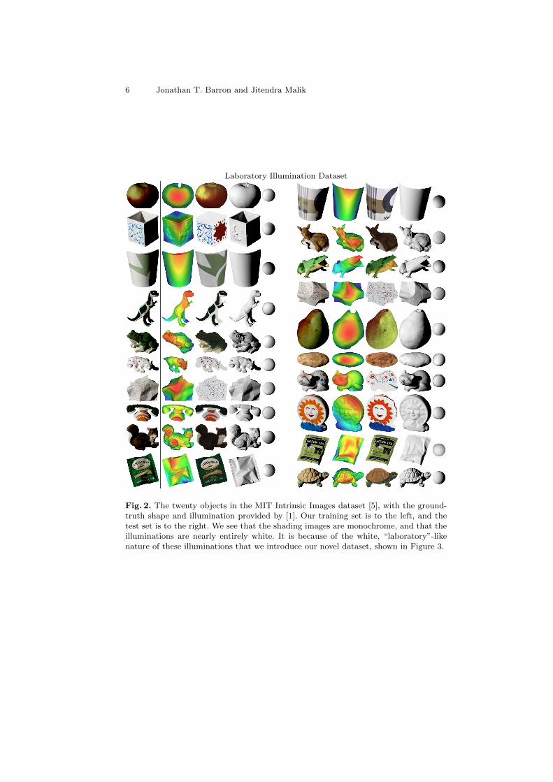
Fig. 2. The twenty objects in the MIT Intrinsic Images dataset [5], with the ground-truth shape and illumination provided by [1]. Our training set is to the left, and thetest set is to the right. We see that the shading images are monochrome, and that theilluminations are nearly entirely white. It is because of the white, “laboratory”-likenature of these illuminations that we introduce our novel dataset, shown in Figure 3.


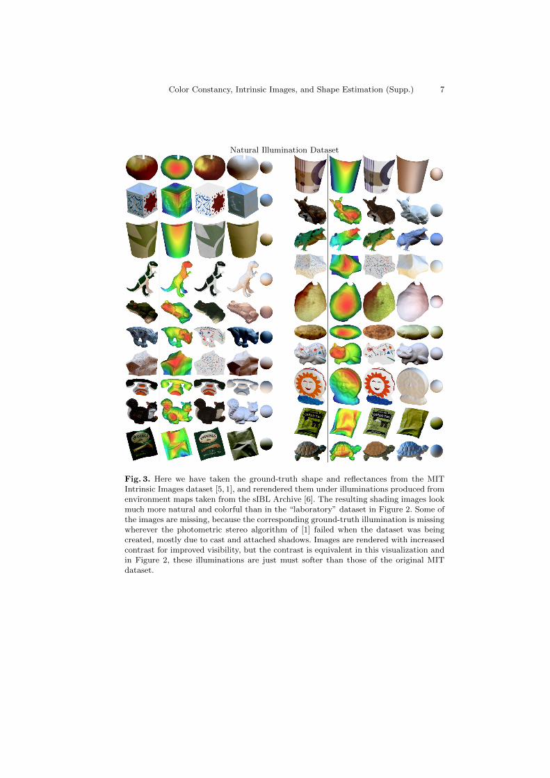
Natural Illumination Dataset

Fig. 3. Here we have taken the ground-truth shape and reflectances from the MITIntrinsic Images dataset [5, 1], and rerendered them under illuminations produced fromenvironment maps taken from the sIBL Archive [6]. The resulting shading images lookmuch more natural and colorful than in the “laboratory” dataset in Figure 2. Some ofthe images are missing, because the corresponding ground-truth illumination is missingwherever the photometric stereo algorithm of [1] failed when the dataset was beingcreated, mostly due to cast and attached shadows. Images are rendered with increasedcontrast for improved visibility, but the contrast is equivalent in this visualization andin Figure 2, these illuminations are just must softer than those of the original MITdataset.


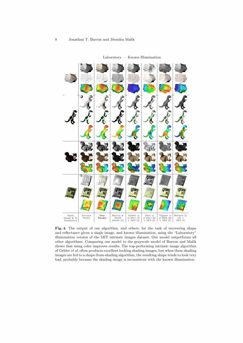
Laboratory — Known Illumination

InputImage & Il-lumination

GroundTruth

OurModel

Barron &Malik

2012A [1]

Gehler etal.2011 [7]+ SFS [1]

Shen etal.2011 [8]+ SFS [1]

Tappen etal.2005 [9]+ SFS [1]

Retinex [5,10] +

SFS [1]

Fig. 4. The output of our algorithm, and others, for the task of recovering shapeand reflectance given a single image, and known illumination, using the “Laboratory”illumination version of the MIT intrinsic images dataset. Our model outperforms allother algorithms. Comparing our model to the grayscale model of Barron and Malikshows that using color improves results. The top-performing intrinsic image algorithmof Gehler et al. often produces excellent looking shading images, but when these shadingimages are fed to a shape-from-shading algorithm, the resulting shape tends to look verybad, probably because the shading image is inconsistent with the known illumination.


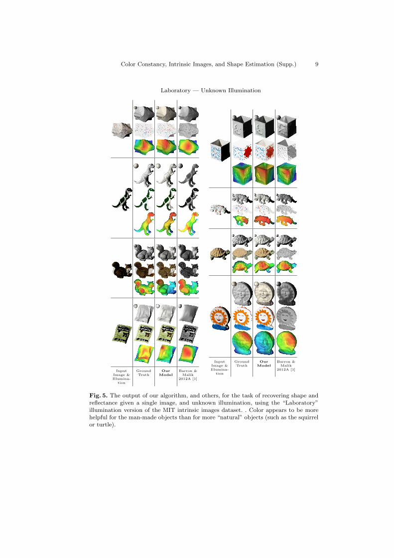
Laboratory — Unknown Illumination

InputImage &Illumina-

tion

GroundTruth

OurModel

Barron &Malik

2012A [1]


tion

GroundTruth

OurModel

Barron &Malik

2012A [1]

Fig. 5. The output of our algorithm, and others, for the task of recovering shape andreflectance given a single image, and unknown illumination, using the “Laboratory”illumination version of the MIT intrinsic images dataset. . Color appears to be morehelpful for the man-made objects than for more “natural” objects (such as the squirrelor turtle).


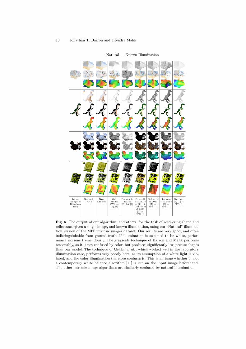
Natural — Known Illumination


tion

GroundTruth

OurModel

OurModel(WhiteLight)

Barron &Malik

2012A [1]

Gijsenijet al.2010+ [11] +Gehler etal.2011[7] +

SFS [1]

Gehler etal.2011[7] +

SFS [1]

Tappenet al.2005

[9] +SFS [1]

Retinex[5, 10] +SFS [1]

Fig. 6. The output of our algorithm, and others, for the task of recovering shape andreflectance given a single image, and known illumination, using our “Natural” illumina-tion version of the MIT intrinsic images dataset. Our results are very good, and oftenindistinguishable from ground-truth. If illumination is assumed to be white, perfor-mance worsens tremendously. The grayscale technique of Barron and Malik performsreasonably, as it is not confused by color, but produces significantly less precise shapesthan our model. The technique of Gehler et al. , which worked well in the laboratoryillumination case, performs very poorly here, as its assumption of a white light is vio-lated, and the color illumination therefore confuses it. This is an issue whether or nota contemporary white balance algorithm [11] is run on the input image beforehand.The other intrinsic image algorithms are similarly confused by natural illumination.


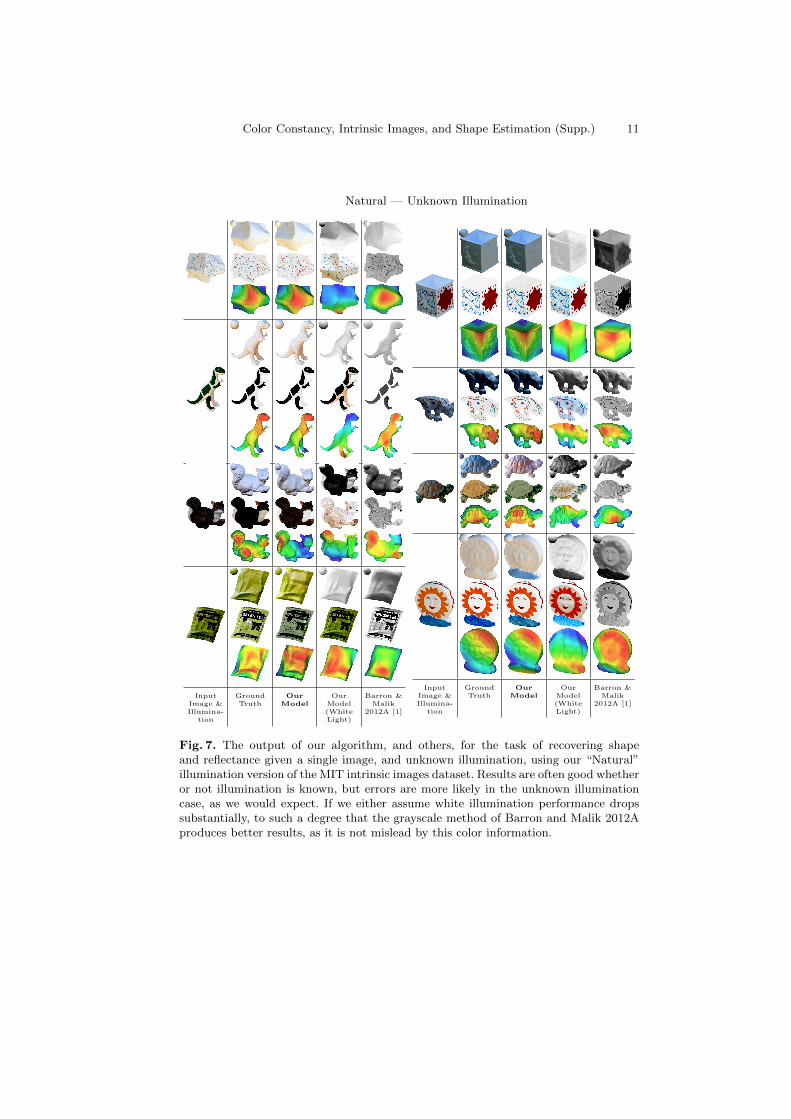
Natural — Unknown Illumination


tion

GroundTruth

OurModel


Barron &Malik

2012A [1]


tion

GroundTruth

OurModel


Barron &Malik

2012A [1]

Fig. 7. The output of our algorithm, and others, for the task of recovering shapeand reflectance given a single image, and unknown illumination, using our “Natural”illumination version of the MIT intrinsic images dataset. Results are often good whetheror not illumination is known, but errors are more likely in the unknown illuminationcase, as we would expect. If we either assume white illumination performance dropssubstantially, to such a degree that the grayscale method of Barron and Malik 2012Aproduces better results, as it is not mislead by this color information.


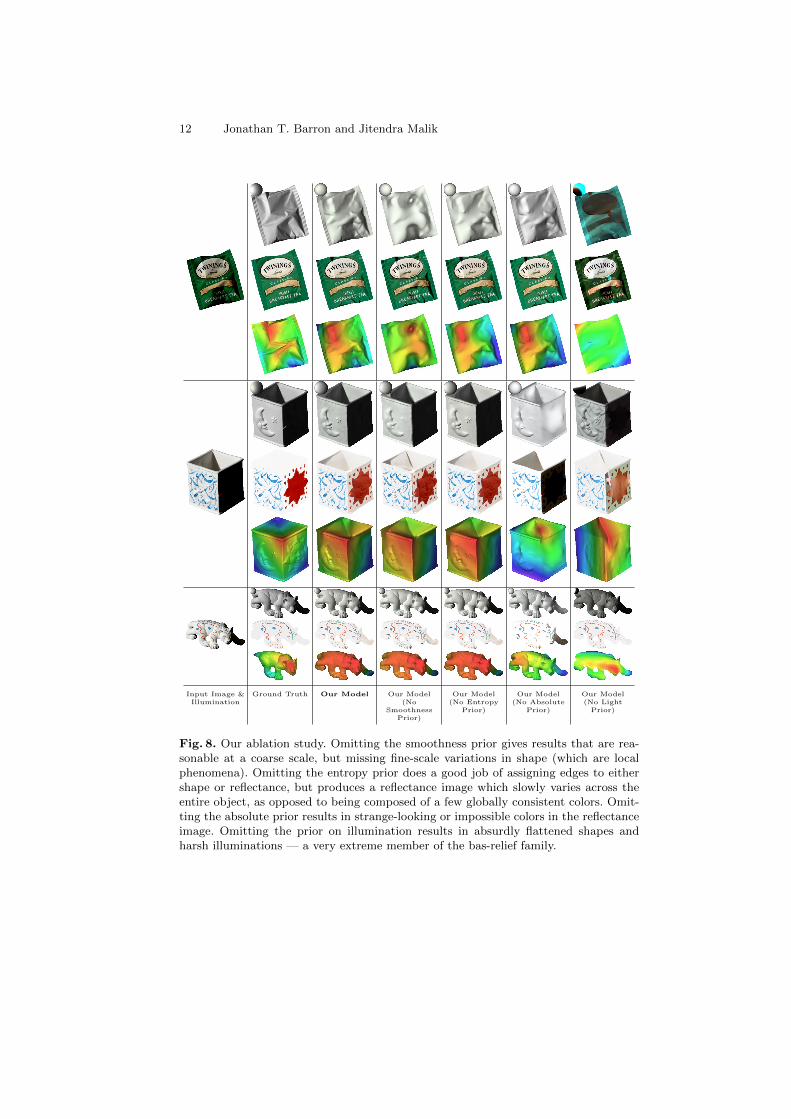
Input Image &Illumination

Ground Truth Our Model Our Model(No

SmoothnessPrior)

Our Model(No Entropy

Prior)

Our Model(No Absolute

Prior)

Our Model(No Light

Prior)

Fig. 8. Our ablation study. Omitting the smoothness prior gives results that are rea-sonable at a coarse scale, but missing fine-scale variations in shape (which are localphenomena). Omitting the entropy prior does a good job of assigning edges to eithershape or reflectance, but produces a reflectance image which slowly varies across theentire object, as opposed to being composed of a few globally consistent colors. Omit-ting the absolute prior results in strange-looking or impossible colors in the reflectanceimage. Omitting the prior on illumination results in absurdly flattened shapes andharsh illuminations — a very extreme member of the bas-relief family.

Color Constancy, Intrinsic Images, and Shape Estimation ......Jonathan T. Barron and Jitendra Malik...

Documents

Transcript of Color Constancy, Intrinsic Images, and Shape Estimation ......Jonathan T. Barron and Jitendra Malik...