arX

iv:m

ath/

0208

140v

3 [

mat

h.Q

A]

21

Aug

200

3

Coideal subalgebras in quantum affine algebras

A. I. Molev, E. Ragoucy and P. Sorba

Abstract

We introduce two subalgebras in the type A quantum affine algebra which

are coideals with respect to the Hopf algebra structure. In the classical limit

q → 1 each subalgebra specializes to the enveloping algebra U(k), where k

is a fixed point subalgebra of the loop algebra glN [λ, λ−1] with respect to a

natural involution corresponding to the embedding of the orthogonal or sym-

plectic Lie algebra into glN . We also give an equivalent presentation of these

coideal subalgebras in terms of generators and defining relations which have

the form of reflection-type equations. We provide evaluation homomorphisms

from these algebras to the twisted quantized enveloping algebras introduced

earlier by Gavrilik and Klimyk and by Noumi. We also construct an analog of

the quantum determinant for each of the algebras and show that its coefficients

belong to the center of the algebra. Their images under the evaluation homo-

morphism provide a family of central elements of the corresponding twisted

quantized enveloping algebra.

Preprint LAPTH-927/02

School of Mathematics and Statistics

University of Sydney, NSW 2006, Australia

alexm@maths.usyd.edu.au

LAPTH, Chemin de Bellevue, BP 110

F-74941 Annecy-le-Vieux cedex, France

ragoucy@lapp.in2p3.fr

LAPTH, Chemin de Bellevue, BP 110

F-74941 Annecy-le-Vieux cedex, France

sorba@lapp.in2p3.fr

1

1 Introduction

For a simple Lie algebra g over C consider the corresponding quantized enveloping

algebra Uq(g); see Drinfeld [9], Jimbo [18]. If k is a subalgebra of g then U(k) is a Hopf

subalgebra of U(g). However, Uq(k), even when it is defined, need not be isomorphic

to a Hopf subalgebra of Uq(g). In the case where (g, k) is a classical symmetric

pair the twisted quantized enveloping algebra Utwq (k) was introduced by Noumi [31]

(type A pairs) and by Noumi and Sugitani [32] (remaining classical types). This is

a subalgebra and a left coideal of the Hopf algebra Uq(g) which specializes to U(k)

as q → 1. The algebras Utwq (k) play an important role in the theory of quantum

symmetric spaces developed in [31] and [32]. In particular, in the type A, which we

are only concerned with in this paper, there are two twisted quantized enveloping

algebras Utwq (oN) and Utw

q (sp2n) corresponding to the symmetric pairs

AI : (glN , oN),

AII : (gl2n, sp2n),(1.1)

respectively. It was also shown by Noumi [31] that the algebra Utwq (oN) coincides with

the one introduced earlier by Gavrilik and Klimyk [12]. The algebra Utwq (oN) also

appears as the symmetry algebra for the q-oscillator representation of the quantized

enveloping algebra Uq(sp2n); see Noumi, Umeda and Wakayama [33, 34].

In Noumi’s approach, the defining relations for the quantized algebras can be

written in the form of a reflection-type equation. A constant solution of the reflection

equation provides an embedding of the twisted quantized enveloping algebra into

Uq(glN). The quantum homogeneous spaces corresponding to the remaining series of

the classical symmetric pairs of type A

AIII : (glN , glN−l ⊕ gl l) (1.2)

were studied by Dijkhuizen, Noumi and Sugitani [6], [7]. A one-parameter family of

the constant solutions of the appropriate reflection equation was produced in [7], al-

though no reflection-type presentation of the subalgebras of type Utwq (k) were formally

introduced.

A different description of the coideal subalgebras of Uq(g) associated with an arbi-

trary irreducible symmetric pair (g, k) was given by Letzter [22, 23]. The subalgebras

are presented by generators and explicit relations depending on the Cartan matrix

of g; see [23]. In particular, this work demonstrates the importance of the coideal

property: it makes the construction of the twisted quantized algebras essentially

unique.

Natural infinite-dimensional analogs of the symmetric pairs are provided by in-

volutive subalgebras in the polynomial current Lie algebras g[x] = g ⊗ C[x] or loop

2

algebras g[λ, λ−1] = g⊗C[λ, λ−1]. Let (g, k) be a symmetric pair and g = k⊕p be the

decomposition determined by the involution θ of g. So, k and p are the eigenspaces of

θ with the eigenvalues 1 and −1, respectively. Then the twisted polynomial current

Lie algebra g[x]θ can be defined by

g[x]θ = k⊕ px⊕ kx2 ⊕ px3 ⊕ · · · , (1.3)

or, equivalently, it is the fixed point subalgebra of g[x] with respect to the extension

of θ given by

θ : Axp 7→ (−1)p θ(A)xp, A ∈ g. (1.4)

As it was demonstrated by Drinfeld [9], the enveloping algebra U(g[x]) admits a

canonical deformation in the class of Hopf algebras. The corresponding “quantum”

algebra is called the Yangian and denoted by Y(g). For the case where θ is an

involution of glN corresponding to the pair of type AI or AII, quantum analogs of

the symmetric pairs (glN [x], glN [x]θ) are provided by the Olshanski twisted Yangians

[35]. These are coideal subalgebras in the Yangian Y(glN) and each of them is a

deformation of the enveloping algebra U(glN [x]θ).

In the AIII case, the quantum analogs of the pairs (glN [x], glN [x]θ) are provided

by the reflection algebras B(N, l) which are coideal subalgebras of Y(glN) originally

introduced by Sklyanin [37]. Recently, these algebras and their representations were

studied in connection with the NLS model ; see Liguori, Mintchev and Zhao [24],

Mintchev, Ragoucy and Sorba [25], Molev and Ragoucy [29].

For the symmetric pairs (g[x], g[x]θ) of general types the corresponding coideal

subalgebras in the Yangian Y(g) were recently introduced by Delius, MacKay and

Short [4] in relation with the principal chiral models with boundaries. These subal-

gebras are given in terms of the Q-presentation of the Yangian. A different R-matrix

presentation of coideal subalgebras in the (super) Yangian Y(g) is given by Arnaudon,

Avan, Crampe, Frappat and Ragoucy [1]. Field theoretical applications of the coideal

subalgebras in the quantum affine algebras have been studied in a recent paper by

Delius and MacKay [5].

In the case of the loop algebra g = g[λ, λ−1] there is another natural way (cf.

(1.4)) to extend the involution θ of g,

θ : Aλp 7→ θ(A)λ−p, A ∈ g (1.5)

and thus to define the fixed point subalgebra g θ. In this paper we introduce cer-

tain quantizations of the symmetric pairs (glN , glθ

N) associated with the involution

θ corresponding to the pairs AI and AII. We define the twisted q-Yangians Ytwq (oN)

and Ytwq (sp2n) as subalgebras of the quantum affine algebra Uq(glN). They are left

coideals with respect to the coproduct on Uq(glN ) and specialize to U(glθ

N ) as q → 1.

3

At this point we consider it necessary to comment on the terminology. Although,

as we have mentioned above, the Lie algebra glθ

N is not a “twisted” quantum affine

algebra in the usual meaning, we believe the names we use for the coideal subalgebras

can be justified having in mind their analogy with both the twisted Yangians and the

q-Yangian; cf. [30]. The latter is a subalgebra of the quantum affine algebra Uq(glN )

which can be regarded as a q-analog of the usual Yangian Y(glN); see also Section 3

below.

Our first main result is a construction of the evaluation homomorphisms

Ytwq (oN) → Utw

q (oN), Ytwq (sp2n) → Utw

q (sp2n) (1.6)

to the corresponding twisted quantized enveloping algebras of [12] and [31]. Note that

an evaluation homomorphism Uq( g) → Uq(g) from the quantum affine algebra to the

corresponding quantized enveloping algebra only exists if g is of A type, and the same

holds for the case of the Yangians; see Jimbo [19], Drinfeld [9]. In both the cases the

evaluation homomorphisms play an important role in the representation theory of the

quantum algebras; see Chari and Pressley [2]. An evaluation homomorphism from

the twisted Yangian to the corresponding enveloping algebra U(oN) or U(sp2n) does

exist (see [35], [28]) and has many applications in the classical representation theory;

see e.g. [27] for an overview. Note also that the existence of the homomorphisms

(1.6) is not directly related with the corresponding fact for the A type algebras but

is quite a nontrivial property of the reflection equations satisfied by the generators of

the twisted q-Yangians.

Next we construct an analog of the quantum determinant for each twisted q-

Yangian and show that its coefficients belong to the center of this algebra. The ap-

plication of the evaluation homomorphism (1.6) yields a family of central elements in

Utwq (oN) and Utw

q (sp2n). In the orthogonal case we also produce a ‘short’ determinant-

like formula for this analog which employs a certain map from the symmetric group

into itself. This same map was used in the short formulas for the Sklyanin determi-

nants for the twisted Yangians; see [27]. Some other families of Casimir elements were

constructed by Noumi, Umeda and Wakayama [34] and by Gavrilik and Iorgov [13].

It would be interesting to understand the relationship between the families, as well

as to investigate possible applications to the study of the quantum Howe dual pairs;

cf. [33, 34].

Another intriguing problem is to construct coideal subalgebras of Uq(glN ) of type

AIII, i.e., to find q-analogs of the Sklyanin reflection algebras B(N, l) mentioned

above.

We are grateful to Gustav Delius, Masatoshi Noumi and Toru Umeda for valu-

able discussions. The financial support of the Australian Research Council and the

4

Laboratoire d’Annecy-le-Vieux de Physique Theorique is acknowledged.

2 Coideal subalgebras of Uq(glN)

We shall use an R-matrix presentation of the algebra Uq(glN). Our main references

are Jimbo [19] and Reshetikhin, Takhtajan and Faddeev [36]. We fix a complex

parameter q which is nonzero and not a root of unity. Consider the R-matrix

R = q∑

i

Eii ⊗ Eii +∑

i 6=j

Eii ⊗ Ejj + (q − q−1)∑

i<j

Eij ⊗Eji (2.1)

which is an element of EndCN ⊗EndCN , where the Eij denote the standard matrix

units and the indices run over the set {1, . . . , N}. The R-matrix satisfies the Yang–

Baxter equation

R12 R13R23 = R23 R13 R12, (2.2)

where both sides take values in EndCN ⊗ EndCN ⊗ EndCN and the subindices

indicate the copies of EndCN , e.g., R12 = R⊗ 1 etc.

The quantized enveloping algebra Uq(glN) is generated by elements tij and tij with

1 ≤ i, j ≤ N subject to the relations1

tij = tji = 0, 1 ≤ i < j ≤ N,

tii tii = tii tii = 1, 1 ≤ i ≤ N,

RT1T2 = T2T1R, RT 1T 2 = T 2T 1R, RT 1T2 = T2T 1R.

(2.3)

Here T and T are the matrices

T =∑

i,j

tij ⊗ Eij, T =∑

i,j

tij ⊗Eij , (2.4)

which are regarded as elements of the algebra Uq(glN)⊗EndCN . Both sides of each

of the R-matrix relations in (2.3) are elements of Uq(glN )⊗ EndCN ⊗ EndCN and

the subindices of T and T indicate the copies of EndCN where T or T acts; e.g.

T1 = T ⊗ 1. In terms of the generators the defining relations between the tij can be

written as

qδij tia tjb − qδab tjb tia = (q − q−1) (δb<a − δi<j) tja tib, (2.5)

where δi<j equals 1 if i < j and 0 otherwise. The relations between the tij are

obtained by replacing tij by tij everywhere in (2.5). Finally, the relations involving

both tij and tij have the form

qδij tia tjb − qδab tjb tia = (q − q−1) (δb<a tja tib − δi<j tja tib). (2.6)

1Our T and T correspond to the L-operators L− and L+, respectively, in the notation of [36].

5

We shall also use another R-matrix R given by

R = q−1∑

i

Eii ⊗Eii +∑

i 6=j

Eii ⊗Ejj + (q−1 − q)∑

i>j

Eij ⊗ Eji. (2.7)

We have the relations

R− R = (q − q−1)P, R = PR−1P, (2.8)

where

P =∑

i,j

Eij ⊗Eji (2.9)

is the permutation operator. The following relations are implied by (2.3)

R T1T2 = T2T1R, R T 1T 2 = T 2T 1R, R T1T 2 = T 2T1R. (2.10)

The coproduct ∆ on Uq(glN) is defined by the relations

∆(tij) =

N∑

k=1

tik ⊗ tkj, ∆(tij) =

N∑

k=1

tik ⊗ tkj. (2.11)

It is well known that the algebra Uq(glN) specializes to U(glN) as q → 1. To make

this more precise, regard q as a formal variable and Uq(glN) as an algebra over C(q).

Then set A = C[q, q−1] and consider the A-subalgebra UA of Uq(glN) generated by

the elements

τij =tij

q − q−1for i > j, τij =

tijq − q−1

for i < j, (2.12)

and

τii =tii − 1

q − 1, τii =

tii − 1

q − 1, (2.13)

for i = 1, . . . , N . Then we have an isomorphism

UA ⊗A C ∼= U(glN) (2.14)

with the action of A on C defined via the evaluation q = 1; see e.g. [2, Section 9.2].

Note that τij and τij respectively specialize to the elements Eij and −Eij of U(glN ).

More generally, given a subalgebra V of Uq(glN ), set VA = V ∩ UA. Following

Letzter [22, Section 1], we shall say that V specializes to the subalgebra V ◦ of U(glN )

(as q goes to 1) if the image of VA in UA ⊗A C is V ◦.

6

2.1 Orthogonal case

Following Noumi [31], we introduce the twisted quantized enveloping algebra Utwq (oN)

as the subalgebra of Uq(glN) generated by the matrix elements of the matrix S =

T Tt. It can be easily derived from (2.3) (see [31]) that the matrix S satisfies the

relations

sij = 0, 1 ≤ i < j ≤ N, (2.15)

sii = 1, 1 ≤ i ≤ N, (2.16)

RS1RtS2 = S2R

tS1R, (2.17)

where R t := R t1 denotes the element obtained from R by the transposition in the

first tensor factor:

R t = q∑

i

Eii ⊗ Eii +∑

i 6=j

Eii ⊗Ejj + (q − q−1)∑

i<j

Eji ⊗ Eji. (2.18)

Indeed, the only nontrivial part of this derivation is to verify that

RT1 Tt

1Rt T2 T

t

2 = T2 Tt

2Rt T1 T

t

1R. (2.19)

However, this is implied by the relation RR t = R tR and the following consequences

of (2.3):

Tt

1Rt T2 = T2R

t Tt

1, R Tt

1Tt

2 = Tt

2Tt

1R. (2.20)

We now prove an auxiliary lemma which establishes a weak form of the Poincare–

Birkhoff–Witt theorem for abstract algebras defined by the relation (2.17). It will be

used in both the orthogonal and symplectic cases.

Lemma 2.1. Consider the associative algebra with N2 generators sij, i, j = 1, . . . , N

and the defining relations written in terms of the matrix S = (sij) by the relation

(2.17). Then the ordered monomials of the form

sk1111 sk1212 · · · sk1N1N · · · skN1N1 skN2

N2 · · · skNN

NN (2.21)

with nonnegative powers kij linearly span the algebra.

Proof. Rewriting (2.17) in terms of the generators we get

qδaj+δij sia sjb − qδab+δib sjb sia = (q − q−1) qδai (δb<a − δi<j) sja sib

+ (q − q−1)(qδab δb<i sji sba − qδij δa<j sij sab

)

+ (q − q−1)2 (δb<a<i − δa<i<j) sji sab,

(2.22)

7

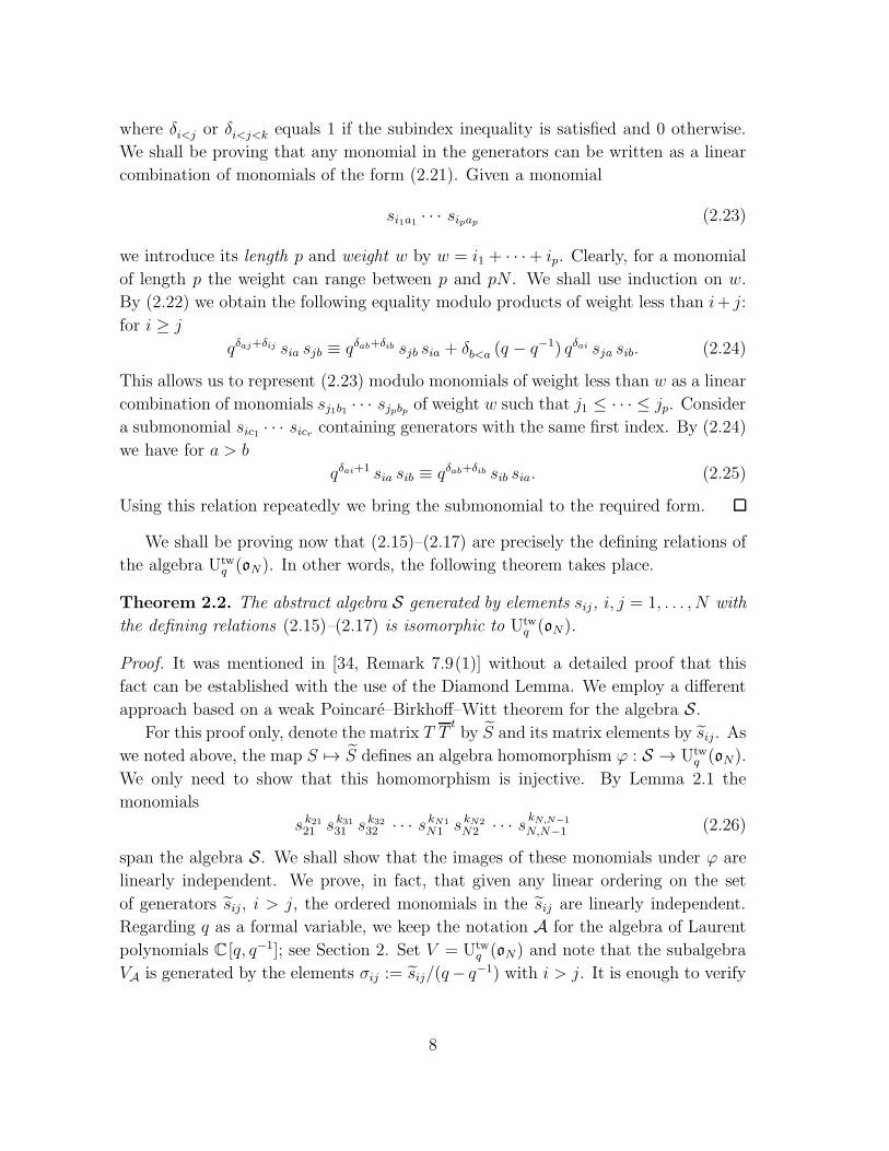
where δi<j or δi<j<k equals 1 if the subindex inequality is satisfied and 0 otherwise.

We shall be proving that any monomial in the generators can be written as a linear

combination of monomials of the form (2.21). Given a monomial

si1a1 · · · sipap (2.23)

we introduce its length p and weight w by w = i1 + · · ·+ ip. Clearly, for a monomial

of length p the weight can range between p and pN . We shall use induction on w.

By (2.22) we obtain the following equality modulo products of weight less than i+ j:

for i ≥ j

qδaj+δij sia sjb ≡ qδab+δib sjb sia + δb<a (q − q−1) qδai sja sib. (2.24)

This allows us to represent (2.23) modulo monomials of weight less than w as a linear

combination of monomials sj1b1 · · · sjpbp of weight w such that j1 ≤ · · · ≤ jp. Consider

a submonomial sic1 · · · sicr containing generators with the same first index. By (2.24)

we have for a > b

qδai+1 sia sib ≡ qδab+δib sib sia. (2.25)

Using this relation repeatedly we bring the submonomial to the required form.

We shall be proving now that (2.15)–(2.17) are precisely the defining relations of

the algebra Utwq (oN). In other words, the following theorem takes place.

Theorem 2.2. The abstract algebra S generated by elements sij, i, j = 1, . . . , N with

the defining relations (2.15)–(2.17) is isomorphic to Utwq (oN).

Proof. It was mentioned in [34, Remark 7.9(1)] without a detailed proof that this

fact can be established with the use of the Diamond Lemma. We employ a different

approach based on a weak Poincare–Birkhoff–Witt theorem for the algebra S.

For this proof only, denote the matrix T Ttby S and its matrix elements by sij. As

we noted above, the map S 7→ S defines an algebra homomorphism ϕ : S → Utwq (oN).

We only need to show that this homomorphism is injective. By Lemma 2.1 the

monomials

s k2121 s k31

31 s k3232 · · · s kN1

N1 s kN2N2 · · · s

kN,N−1

N,N−1 (2.26)

span the algebra S. We shall show that the images of these monomials under ϕ are

linearly independent. We prove, in fact, that given any linear ordering on the set

of generators sij, i > j, the ordered monomials in the sij are linearly independent.

Regarding q as a formal variable, we keep the notation A for the algebra of Laurent

polynomials C[q, q−1]; see Section 2. Set V = Utwq (oN) and note that the subalgebra

VA is generated by the elements σij := sij/(q− q−1) with i > j. It is enough to verify

8

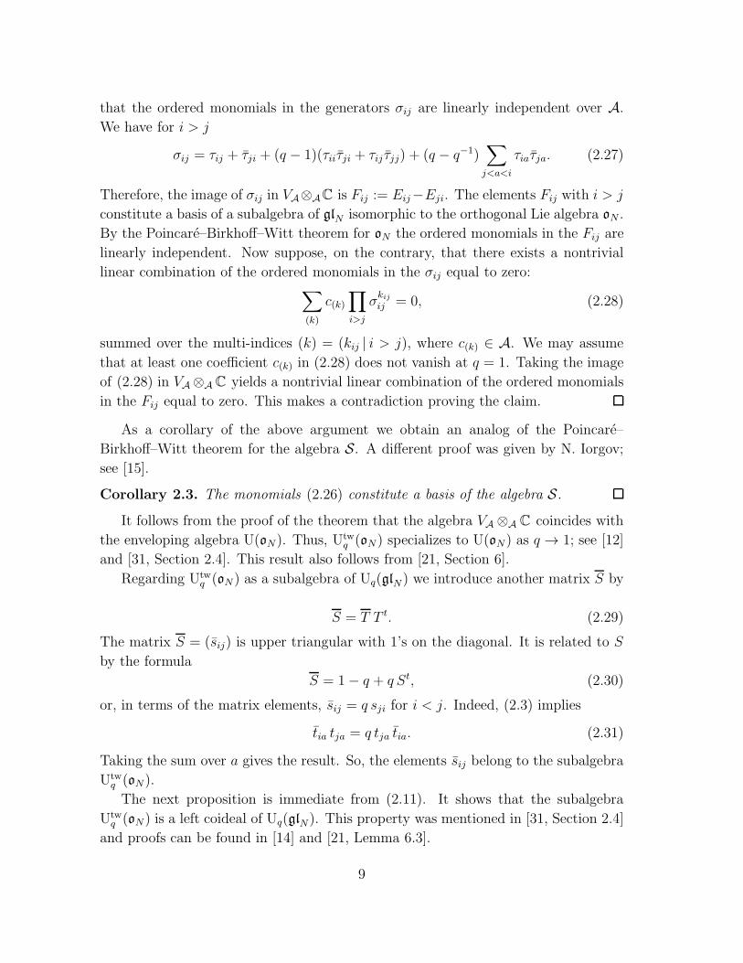
that the ordered monomials in the generators σij are linearly independent over A.

We have for i > j

σij = τij + τji + (q − 1)(τiiτji + τij τjj) + (q − q−1)∑

j<a<i

τiaτja. (2.27)

Therefore, the image of σij in VA⊗AC is Fij := Eij−Eji. The elements Fij with i > j

constitute a basis of a subalgebra of glN isomorphic to the orthogonal Lie algebra oN .

By the Poincare–Birkhoff–Witt theorem for oN the ordered monomials in the Fij are

linearly independent. Now suppose, on the contrary, that there exists a nontrivial

linear combination of the ordered monomials in the σij equal to zero:∑

(k)

c(k)∏

i>j

σkijij = 0, (2.28)

summed over the multi-indices (k) = (kij | i > j), where c(k) ∈ A. We may assume

that at least one coefficient c(k) in (2.28) does not vanish at q = 1. Taking the image

of (2.28) in VA⊗AC yields a nontrivial linear combination of the ordered monomials

in the Fij equal to zero. This makes a contradiction proving the claim.

As a corollary of the above argument we obtain an analog of the Poincare–

Birkhoff–Witt theorem for the algebra S. A different proof was given by N. Iorgov;

see [15].

Corollary 2.3. The monomials (2.26) constitute a basis of the algebra S.

It follows from the proof of the theorem that the algebra VA ⊗A C coincides with

the enveloping algebra U(oN). Thus, Utwq (oN) specializes to U(oN) as q → 1; see [12]

and [31, Section 2.4]. This result also follows from [21, Section 6].

Regarding Utwq (oN) as a subalgebra of Uq(glN) we introduce another matrix S by

S = T T t. (2.29)

The matrix S = (sij) is upper triangular with 1’s on the diagonal. It is related to S

by the formula

S = 1− q + q St, (2.30)

or, in terms of the matrix elements, sij = q sji for i < j. Indeed, (2.3) implies

tia tja = q tja tia. (2.31)

Taking the sum over a gives the result. So, the elements sij belong to the subalgebra

Utwq (oN).

The next proposition is immediate from (2.11). It shows that the subalgebra

Utwq (oN) is a left coideal of Uq(glN). This property was mentioned in [31, Section 2.4]

and proofs can be found in [14] and [21, Lemma 6.3].

9

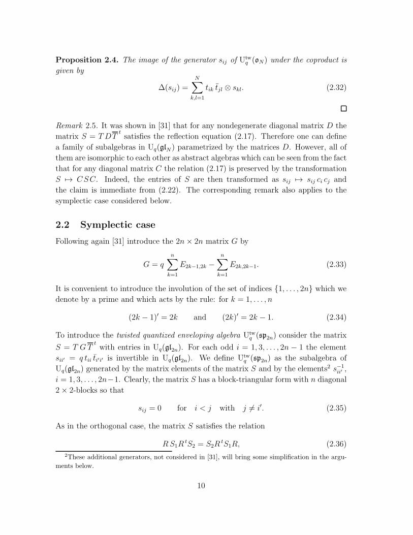
Proposition 2.4. The image of the generator sij of Utwq (oN) under the coproduct is

given by

∆(sij) =

N∑

k,l=1

tik tjl ⊗ skl. (2.32)

Remark 2.5. It was shown in [31] that for any nondegenerate diagonal matrix D the

matrix S = T DTtsatisfies the reflection equation (2.17). Therefore one can define

a family of subalgebras in Uq(glN ) parametrized by the matrices D. However, all of

them are isomorphic to each other as abstract algebras which can be seen from the fact

that for any diagonal matrix C the relation (2.17) is preserved by the transformation

S 7→ CSC. Indeed, the entries of S are then transformed as sij 7→ sij ci cj and

the claim is immediate from (2.22). The corresponding remark also applies to the

symplectic case considered below.

2.2 Symplectic case

Following again [31] introduce the 2n× 2n matrix G by

G = q

n∑

k=1

E2k−1,2k −

n∑

k=1

E2k,2k−1. (2.33)

It is convenient to introduce the involution of the set of indices {1, . . . , 2n} which we

denote by a prime and which acts by the rule: for k = 1, . . . , n

(2k − 1)′ = 2k and (2k)′ = 2k − 1. (2.34)

To introduce the twisted quantized enveloping algebra Utwq (sp2n) consider the matrix

S = T GTtwith entries in Uq(gl2n). For each odd i = 1, 3, . . . , 2n − 1 the element

sii′ = q tii ti′i′ is invertible in Uq(gl2n). We define Utwq (sp2n) as the subalgebra of

Uq(gl2n) generated by the matrix elements of the matrix S and by the elements2 s−1ii′ ,

i = 1, 3, . . . , 2n−1. Clearly, the matrix S has a block-triangular form with n diagonal

2× 2-blocks so that

sij = 0 for i < j with j 6= i′. (2.35)

As in the orthogonal case, the matrix S satisfies the relation

RS1RtS2 = S2R

tS1R, (2.36)

2These additional generators, not considered in [31], will bring some simplification in the argu-

ments below.

10

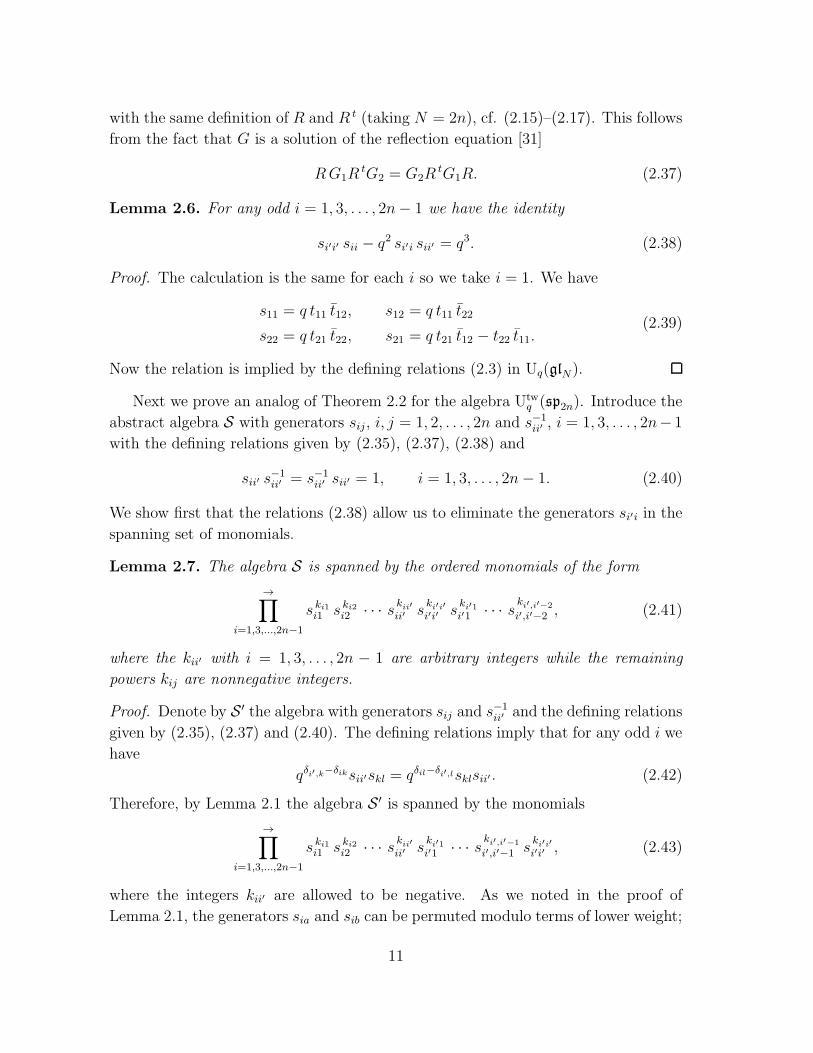
with the same definition of R and R t (taking N = 2n), cf. (2.15)–(2.17). This follows

from the fact that G is a solution of the reflection equation [31]

RG1RtG2 = G2R

tG1R. (2.37)

Lemma 2.6. For any odd i = 1, 3, . . . , 2n− 1 we have the identity

si′i′ sii − q2 si′i sii′ = q3. (2.38)

Proof. The calculation is the same for each i so we take i = 1. We have

s11 = q t11 t12, s12 = q t11 t22

s22 = q t21 t22, s21 = q t21 t12 − t22 t11.(2.39)

Now the relation is implied by the defining relations (2.3) in Uq(glN).

Next we prove an analog of Theorem 2.2 for the algebra Utwq (sp2n). Introduce the

abstract algebra S with generators sij, i, j = 1, 2, . . . , 2n and s−1ii′ , i = 1, 3, . . . , 2n− 1

with the defining relations given by (2.35), (2.37), (2.38) and

sii′ s−1ii′ = s−1

ii′ sii′ = 1, i = 1, 3, . . . , 2n− 1. (2.40)

We show first that the relations (2.38) allow us to eliminate the generators si′i in the

spanning set of monomials.

Lemma 2.7. The algebra S is spanned by the ordered monomials of the form

→∏

i=1,3,...,2n−1

s ki1i1 s ki2

i2 · · · skii′ii′ s

ki′i′i′i′ s

ki′1i′1 · · · s

ki′,i′−2

i′,i′−2 , (2.41)

where the kii′ with i = 1, 3, . . . , 2n − 1 are arbitrary integers while the remaining

powers kij are nonnegative integers.

Proof. Denote by S ′ the algebra with generators sij and s−1ii′ and the defining relations

given by (2.35), (2.37) and (2.40). The defining relations imply that for any odd i we

have

qδi′,k−δiksii′skl = qδil−δi′,lsklsii′ . (2.42)

Therefore, by Lemma 2.1 the algebra S ′ is spanned by the monomials

→∏

i=1,3,...,2n−1

s ki1i1 s ki2

i2 · · · skii′ii′ s

ki′1i′1 · · · s

ki′,i′−1

i′,i′−1 ski′i′i′i′ , (2.43)

where the integers kii′ are allowed to be negative. As we noted in the proof of

Lemma 2.1, the generators sia and sib can be permuted modulo terms of lower weight;

11

see (2.25). Therefore, rearranging the generators appropriately, we conclude that S ′

is also spanned by the monomials

→∏

i=1,3,...,2n−1

s ki1i1 s ki2

i2 · · · skii′ii′ s

ki′,i′−1

i′,i′−1 ski′i′i′i′ s

ki′1i′1 · · · s

ki′,i′−2

i′,i′−2 . (2.44)

It is a straightforward calculation to derive from the defining relations that the ele-

ments si′i′ sii − q2 si′i sii′ with i = 1, 3, . . . , 2n − 1 are central in the algebra S ′. Let

I be the ideal of S ′ generated by the central elements si′i′ sii − q2 si′i sii′ − q3 for

i = 1, 3, . . . , 2n − 1. We need to show that the quotient S ′/I is spanned by the

monomials (2.41). However, the defining relations between the generators sii, sii′,

si′i and si′i′ do not involve any other generators. In order to complete the proof it is

therefore sufficient to consider the particular case n = 1. We shall show that modulo

the ideal I generated by the central element s22 s11 − q2 s21 s12 − q3 every element

of the algebra S ′ can be written as a linear combination of monomials of the form

s k1111 s k12

12 s k2222 . Let s k11

11 s k1212 s k21

21 s k2222 be an arbitrary monomial of the form (2.44). We

assume k21 ≥ 1 and use induction on k21. Modulo the ideal I we have

s21 ≡ q−2s22 s11 s−112 + q s−1

12 . (2.45)

Therefore, omitting the ordered monomials with smaller powers k21 we have the

relation modulo the ideal I:

s k1111 s k12

12 s k2121 s k22

22 ≡ q−2s k1111 s k12−1

12 s22 s11 sk21−121 s k22

22 . (2.46)

Note that by (2.22) we have the relation

s22 s11 = s11 s22 + (q − q−1)(s212 + q s12 s21). (2.47)

This allows us to bring the right hand side of (2.46) to the form

(1− q−2) s k1111 s k12

12 s k2121 s k22

22 , (2.48)

which completes the proof.

The following is an analog of Theorem 2.2 for the symplectic case.

Theorem 2.8. The algebra S is isomorphic to Utwq (sp2n).

Proof. We use the same argument as for the proof of Theorem 2.2. For this proof

only, denote the matrix T GTtby S and its matrix elements by sij. The map S 7→ S

defines an algebra homomorphism ϕ : S → Utwq (sp2n). We show that the images

of the monomials (2.41) under ϕ are linearly independent. Note that by (2.42) the

12

product of a monomial of the form (2.41) and skii′ is, up to a nonzero factor, equal

to the same monomial with the index kii′ replaced with kii′ + k. Therefore we may

assume without loss of generality that all powers in (2.41) are nonnegative integers.

Set V = Utwq (sp2n). The corresponding generators σij ∈ VA can now be given by

σij =sij − gijq − q−1

, (2.49)

where the gij are the matrix elements of G. We have the relation modulo (q − 1),

σij ≡ gj′j τij′ + gii′ τji′ , (2.50)

where gij is the value of gij at q = 1 so that gii′ = (−1)i−1. Therefore, the image

of the element σij in VA ⊗A C is Fij := gj′j Eij′ − gii′ Eji′. The elements Fij span a

subalgebra of gl2n isomorphic to the symplectic Lie algebra sp2n and this allows us

to complete the proof exactly as in the orthogonal case.

The following is an analog of the Poincare–Birkhoff–Witt theorem for the algebra

S which is immediate from Theorem 2.8.

Corollary 2.9. The monomials (2.41) constitute a basis of the algebra S.

It follows from the proof of the theorem that the algebra VA ⊗A C coincides with

the enveloping algebra U(sp2n). Thus, Utwq (sp2n) specializes to U(sp2n) as q → 1.

The result also follows from [21, Section 6].

Regarding Utwq (sp2n) as a subalgebra of Uq(gl2n) we introduce another matrix S

by

S = T GT t. (2.51)

Using the same argument as in the orthogonal case (see Section 2.1) we derive the

following relations between the matrix elements of S and S: for any i = 1, 3, . . . 2n−1

sii = −q−2 sii, si′i′ = −q−2 si′i′ ,

si′i = −q−1 sii′, sii′ = −q−1 si′i + (1− q−2) sii′,(2.52)

while for the remaining generators we have

sij = −q−1 sji, i < j, j 6= i′. (2.53)

Thus, the elements sij belong to the subalgebra Utwq (sp2n).

The next proposition is immediate from (2.11); cf. Proposition 2.4. It shows that

the subalgebra Utwq (sp2n) is a left coideal of Uq(gl2n); see [21, Lemma 6.3].

13

Proposition 2.10. The images of the generators of Utwq (sp2n) under the coproduct

are given by

∆(sij) =

2n∑

k,l=1

tik tjl ⊗ skl (2.54)

and

∆(s−1ii′ ) = ti′i′ tii ⊗ s−1

ii′ . (2.55)

3 Coideal subalgebras of Uq(glN)

Consider the Lie algebra of Laurent polynomials glN [λ, λ−1] in an indeterminate λ.

We denote it by glN for brevity. The quantum affine algebra Uq(glN) is a deforma-

tion of the universal enveloping algebra U(glN). We use its R-matrix presentation

following Reshetikhin, Takhtajan and Faddeev [36]; cf. Section 2. Note also a recent

work of Frenkel and Mukhin [11], where different realizations of Uq(glN) are collected.

By definition, the algebra Uq(glN ) has countably many generators t(r)ij and t

(r)ij where

1 ≤ i, j ≤ N and r runs over nonnegative integers. They are combined into the

matrices

T (u) =N∑

i,j=1

tij(u)⊗ Eij, T (u) =N∑

i,j=1

tij(u)⊗Eij , (3.1)

where tij(u) and tij(u) are formal series in u−1 and u, respectively:

tij(u) =

∞∑

r=0

t(r)ij u−r, tij(u) =

∞∑

r=0

t(r)ij ur. (3.2)

The defining relations are

t(0)ij = t

(0)ji = 0, 1 ≤ i < j ≤ N,

t(0)ii t

(0)ii = t

(0)ii t

(0)ii = 1, 1 ≤ i ≤ N,

R(u, v) T1(u)T2(v) = T2(v)T1(u)R(u, v),

R(u, v) T 1(u)T 2(v) = T 2(v)T 1(u)R(u, v),

R(u, v) T 1(u)T2(v) = T2(v)T 1(u)R(u, v),

(3.3)

where we have used the notation of (2.3) and R(u, v) is the trigonometric R-matrix

given by

R(u, v) = (u− v)∑

i 6=j

Eii ⊗ Ejj + (q−1u− qv)∑

i

Eii ⊗Eii

+ (q−1 − q)u∑

i>j

Eij ⊗ Eji + (q−1 − q)v∑

i<j

Eij ⊗Eji.(3.4)

14

It satisfies the Yang–Baxter equation

R12(u, v)R13(u, w)R23(v, w) = R23(v, w)R13(u, w)R12(u, v), (3.5)

where both sides take values in EndCN ⊗ EndCN ⊗ EndCN and the subindices

indicate the copies of EndCN , e.g., R12(u, v) = R(u, v)⊗ 1 etc. Note that R(u, v) is

related with the constant R-matrices (2.1) and (2.7) by the formula

R(u, v) = u R− v R. (3.6)

There is a Hopf algebra structure on Uq(glN) with the coproduct defined by

∆(tij(u)

)=

N∑

k=1

tik(u)⊗ tkj(u), ∆(tij(u)

)=

N∑

k=1

tik(u)⊗ tkj(u). (3.7)

The algebra Uq(glN) specializes to U(glN) as q → 1. More precisely, as with

the case of Uq(glN) (see Section 2), regard q as a formal variable and introduce the

A-subalgebra UA of Uq(glN) generated by the elements τ(r)ij and τ

(r)ij defined by

τ(r)ij =

t(r)ij

q − q−1, τ

(r)ij =

t(r)ij

q − q−1(3.8)

for r ≥ 0 and all i, j, except for the case r = 0 and i = j where we set

τ(0)ii =

t(0)ii − 1

q − 1, τ

(0)ii =

t(0)ii − 1

q − 1. (3.9)

Then we have an isomorphism

UA ⊗A C ∼= U(glN ); (3.10)

see [2, Section 12.2] and [11, Section 2]. The images of the generators of UA in (3.10)

are given by

τ(r)ij → Eijλ

r, τ(r)ij → −Eijλ

−r (3.11)

for all r ≥ 0 with the exception τ(0)ij = τ

(0)ji = 0 if i < j. Given a subalgebra V of

Uq(glN) we set VA = V ∩ UA. We shall say that V specializes to a subalgebra V ◦ of

U(glN) if VA ⊗A C ∼= V ◦.

The quantized enveloping algebra Uq(glN ) is a natural (Hopf) subalgebra of

Uq(glN) defined by the embedding

tij 7→ t(0)ij , tij 7→ t

(0)ij . (3.12)

15

Moreover, there is an algebra homomorphism Uq(glN) → Uq(glN ) called the evalua-

tion homomorphism defined by

T (u) 7→ T − T u−1, T (u) 7→ T − T u. (3.13)

The A type quantum affine algebras are exceptional in the sense that only in this case

such an evaluation homomorphism does exist; see Chari–Pressley [2, Chapter 12].

The subalgebra of Uq(glN) generated by the elements t(r)ij was studied e.g. in

[3], [30], [36]. We call it the q-Yangian. In what follows we construct quantum

affine algebras associated with the orthogonal and symplectic Lie algebras for which

analogs of the evaluation homomorphism (3.13) do exist; cf. the B and C type twisted

Yangians [35], [28]. These algebras can be viewed as twisted analogs of the q-Yangian

as well as q-analogs of the twisted Yangians. Note, however, that contrary to the case

of the twisted Yangians, our algebras are not subalgebras of the q-Yangian; they are

generated by certain combinations of both types of elements t(r)ij and t

(r)ij .

3.1 Orthogonal twisted q-Yangians

Definition 3.1. The twisted q-Yangian Ytwq (oN) is the subalgebra of Uq(glN) gener-

ated by the coefficients s(r)ij of the matrix elements of the matrix S(u) = T (u) T (u−1)t.

More precisely, we have

sij(u) =

N∑

a=1

tia(u) tja(u−1) (3.14)

so that

sij(u) =∞∑

r=0

s(r)ij u−r. (3.15)

The subalgebra Ytwq (oN) is generated by the elements s

(r)ij with 1 ≤ i, j ≤ N and r

running over the set of nonnegative integers.

Next we give a presentation of the algebra Ytwq (oN) in terms of generators and

defining relations by analogy with the finite-dimensional case; see Section 2.1. Con-

sider the element R t(u, v) := R t1(u, v) obtained from R(u, v) by the transposition in

the first factor:

R t(u, v) = (u− v)∑

i 6=j

Eii ⊗ Ejj + (q−1u− qv)∑

i

Eii ⊗Eii

+ (q−1 − q)u∑

i>j

Eji ⊗ Eji + (q−1 − q)v∑

i<j

Eji ⊗Eji.(3.16)

16

The following relations are implied by (3.3):

s(0)ij = 0, 1 ≤ i < j ≤ N, (3.17)

s(0)ii = 1, 1 ≤ i ≤ N, (3.18)

R(u, v)S1(u)Rt(u−1, v)S2(v) = S2(v)R

t(u−1, v)S1(u)R(u, v). (3.19)

We shall be proving that these are precisely the defining relations for the algebra

Ytwq (oN).

Lemma 3.2. Consider the (abstract) associative algebra with generators s(r)ij where

i, j = 1, . . . , N and r = 0, 1, . . . . The defining relations are written in terms of the

matrix S(u) = (sij(u)) by the relation (3.19) with sij(u) defined by (3.15). Introduce

the ordering on the generators in such a way that s(r)ij � s

(p)kl if and only if (r, i, j) �

(p, k, l) in the lexicographical order. Then the ordered monomials in the generators

span the algebra.

Proof. Write the defining relations in terms of the generating series sij(u):

(q−δiju− qδijv)αijab(u, v) + (q−1 − q)(uδj<i + vδi<j)αjiab(u, v)

= (q−δabu− qδabv)αjiba(v, u) + (q−1 − q)(uδa<b + vδb<a)αjiab(v, u),(3.20)

where we have used the notation

αijab(u, v) = (q−δaj−qδajuv) sia(u) sjb(v)+(q−1−q)(δj<a+uvδa<j) sij(u) sab(v). (3.21)

We shall show that any monomial

s(k1)i1a1

s(k2)i2a2

· · · s(kp)ipap

(3.22)

can be written as a linear combination of the ordered monomials. Define the degree

of the monomial (3.22) as the sum k1+ · · ·+kp and argue by induction on the degree.

The induction base is Lemma 2.1 which takes care of the monomials of degree zero.

In other words, we can introduce the filtration on the algebra by setting deg s(k)ia = k

and it will be sufficient to prove the lemma for the corresponding graded algebra.

We keep the same notation for its generators while the defining relations are given

by (3.20) where instead of (3.21) we should take

αijab(u, v) = −qδaj sia(u) sjb(v) + (q−1 − q) δa<j sij(u) sab(v). (3.23)

Furthermore, we apply the same argument to this new algebra considering the filtra-

tion defined by setting the degree of s(k)ia to be equal to i. The corresponding graded

17

algebra is generated by elements s(k)ia with the defining relations (3.20) where the

expression αijab(u, v) further simplifies to

αijab(u, v) = −qδaj sia(u) sjb(v). (3.24)

Working with this algebra we have for i > j

qδaj sia(u) sjb(v) =q−δabu− qδabv

u− vqδbi sjb(v) sia(u)

+q − q−1

u− vqδai

(u sja(u) sib(v)− (uδa<b + vδb<a) sja(v) sib(u)

).

(3.25)

This implies that the monomials (3.22) with the condition i1 ≤ · · · ≤ ip span the

algebra. Now we take i = j and a < b in (3.20) with the assumption (3.24) to get

qδbi sib(v) sia(u) =q−1u− q v

q−δabu− qδabvqδai sia(u) sib(v)

+q − q−1

q−δabu− qδabvqδai u sia(v) sib(u).

(3.26)

Therefore, the algebra is spanned by the monomials (3.22) such that (i1, a1) � · · · �

(ip, ap) in the lexicographical order. Finally, using again (3.20) we note that

sia(u) sia(v) = sia(v) sia(u) (3.27)

which implies [s(k)ia , s

(r)ia ] = 0 for all k, r. This completes the proof.

Theorem 3.3. The abstract algebra S generated by elements s(r)ij with i, j = 1, . . . , N

and r ≥ 0 with the defining relations (3.17)–(3.19) is isomorphic to Ytwq (oN).

Proof. We use the argument of the proof of Theorem 2.2 appropriately modified

for the affine case. Namely, we check first that the matrix elements of the matrix

T (u) T (u−1)t satisfy the defining relations of S so that we have an algebra homomor-

phism S → Ytwq (oN). To prove its injectivity regard q as a formal variable and set

V = Ytwq (oN). Note that the algebra VA is generated by the elements

σ(r)ij =

s(r)ij

q − q−1, (3.28)

where the condition i > j must hold if r = 0. The image of σ(r)ij in VA ⊗A C is

F(r)ij = Eijλ

r − Ejiλ−r. However, the elements F

(r)ij span the fixed point subalgebra

glθ

N of glN corresponding to the automorphism

θ : Eij λp 7→ −Eji λ

−p. (3.29)

Thus, Lemma 3.2 and this observation complete the proof.

18

Consider the ordering on the generators of S defined in Lemma 3.2. We shall

assume that for the generators s(0)ij the condition i > j holds.

Corollary 3.4. The ordered monomials in the generators constitute a basis of the

algebra S.

Corollary 3.5. The subalgebra Ytwq (oN) of Uq(glN ) specializes to the universal en-

veloping algebra U(glθ

N) as q → 1.

The following proposition is immediate from (3.7).

Proposition 3.6. The subalgebra Ytwq (oN) of Uq(glN) is a left coideal so that

∆(sij(u)) =N∑

k,l=1

tik(u) tjl(u−1)⊗ skl(u). (3.30)

The next proposition allows us to regard Utwq (oN) as a subalgebra of Ytw

q (oN).

Proposition 3.7. The map sij 7→ s(0)ij defines an embedding Utw

q (oN) → Ytwq (oN).

Proof. It is clear from (3.17)–(3.19) that the elements s(0)ij satisfy the defining rela-

tions for the sij; see (2.15)–(2.17). Corollary 3.4 ensures that the homomorphism is

injective.

The following theorem establishes the existence of the evaluation homomorphisms

for the twisted q-Yangians. We use notation (2.29). As before, we combine the formal

series sij(u) into the matrix S(u) so that S(u) is a formal power series in u−1 with

matrix coefficients.

Theorem 3.8. The mapping

S(u) 7→ S + q−1 u−1 S (3.31)

defines an algebra homomorphism Ytwq (oN) → Utw

q (oN).

Proof. Regarding Ytwq (oN) as an abstract algebra we need to verify that the relation

(3.19) holds when we substitute the right hand side of (3.31) for S(u). That is, we

need to verify

(uR− vR)(q u S1 + S1)(Rt − uvRt)(q v S2 + S2)

= (q v S2 + S2)(Rt − uvRt)(q u S1 + S1)(uR− vR). (3.32)

19

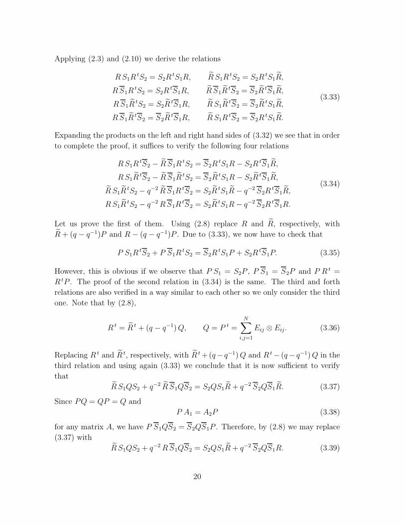
Applying (2.3) and (2.10) we derive the relations

RS1RtS2 = S2R

tS1R, R S1RtS2 = S2R

tS1R,

RS1RtS2 = S2R

tS1R, R S1RtS2 = S2R

tS1R,

R S1RtS2 = S2R

tS1R, R S1RtS2 = S2R

tS1R,

RS1RtS2 = S2R

tS1R, R S1RtS2 = S2R

tS1R.

(3.33)

Expanding the products on the left and right hand sides of (3.32) we see that in order

to complete the proof, it suffices to verify the following four relations

RS1RtS2 − R S1R

tS2 = S2RtS1R − S2R

tS1R,

RS1RtS2 − R S1R

tS2 = S2RtS1R − S2R

tS1R,

R S1RtS2 − q−2 R S1R

tS2 = S2RtS1R− q−2 S2R

tS1R,

R S1RtS2 − q−2RS1R

tS2 = S2RtS1R− q−2 S2R

tS1R.

(3.34)

Let us prove the first of them. Using (2.8) replace R and R, respectively, with

R + (q − q−1)P and R − (q − q−1)P . Due to (3.33), we now have to check that

P S1RtS2 + P S1R

tS2 = S2RtS1P + S2R

tS1P. (3.35)

However, this is obvious if we observe that P S1 = S2P , P S1 = S2P and P R t =

R tP . The proof of the second relation in (3.34) is the same. The third and forth

relations are also verified in a way similar to each other so we only consider the third

one. Note that by (2.8),

R t = R t + (q − q−1)Q, Q = P t =

N∑

i,j=1

Eij ⊗ Eij . (3.36)

Replacing R t and R t, respectively, with R t+(q− q−1)Q and R t− (q− q−1)Q in the

third relation and using again (3.33) we conclude that it is now sufficient to verify

that

R S1QS2 + q−2 R S1QS2 = S2QS1R + q−2 S2QS1R. (3.37)

Since PQ = QP = Q and

P A1 = A2P (3.38)

for any matrix A, we have P S1QS2 = S2QS1P . Therefore, by (2.8) we may replace

(3.37) with

R S1QS2 + q−2RS1QS2 = S2QS1R + q−2 S2QS1R. (3.39)

20

Finally, we have the chain of equalities

R S1Q = R T1Tt

1Q = R T1T 2Q = T 2T1RQ = q−1T 2T1Q = q−1T 2Tt2Q = q−1S2Q,

(3.40)

where we have used (2.10) and the relations R Q = QR = q−1Q together with the

observation that At1Q = A2Q implied by (3.38). Thus, R S1QS2 = q−1S2QS2. A

similar argument shows that

RS1QS2 = q S2QS2, S2QS1R = q−1S2QS2, S2QS1R = q S2QS2 (3.41)

proving (3.39) and the theorem.

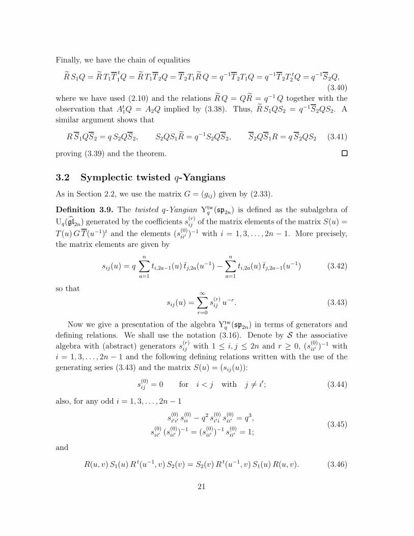
3.2 Symplectic twisted q-Yangians

As in Section 2.2, we use the matrix G = (gij) given by (2.33).

Definition 3.9. The twisted q-Yangian Ytwq (sp2n) is defined as the subalgebra of

Uq(gl2n) generated by the coefficients s(r)ij of the matrix elements of the matrix S(u) =

T (u)GT (u−1)t and the elements (s(0)ii′ )

−1 with i = 1, 3, . . . , 2n − 1. More precisely,

the matrix elements are given by

sij(u) = qn∑

a=1

ti,2a−1(u) tj,2a(u−1)−

n∑

a=1

ti,2a(u) tj,2a−1(u−1) (3.42)

so that

sij(u) =

∞∑

r=0

s(r)ij u−r. (3.43)

Now we give a presentation of the algebra Ytwq (sp2n) in terms of generators and

defining relations. We shall use the notation (3.16). Denote by S the associative

algebra with (abstract) generators s(r)ij with 1 ≤ i, j ≤ 2n and r ≥ 0, (s

(0)ii′ )

−1 with

i = 1, 3, . . . , 2n − 1 and the following defining relations written with the use of the

generating series (3.43) and the matrix S(u) = (sij(u)):

s(0)ij = 0 for i < j with j 6= i′; (3.44)

also, for any odd i = 1, 3, . . . , 2n− 1

s(0)i′i′ s

(0)ii − q2 s

(0)i′i s

(0)ii′ = q3,

s(0)ii′ (s

(0)ii′ )

−1 = (s(0)ii′ )

−1 s(0)ii′ = 1;

(3.45)

and

R(u, v)S1(u)Rt(u−1, v)S2(v) = S2(v)R

t(u−1, v)S1(u)R(u, v). (3.46)

21

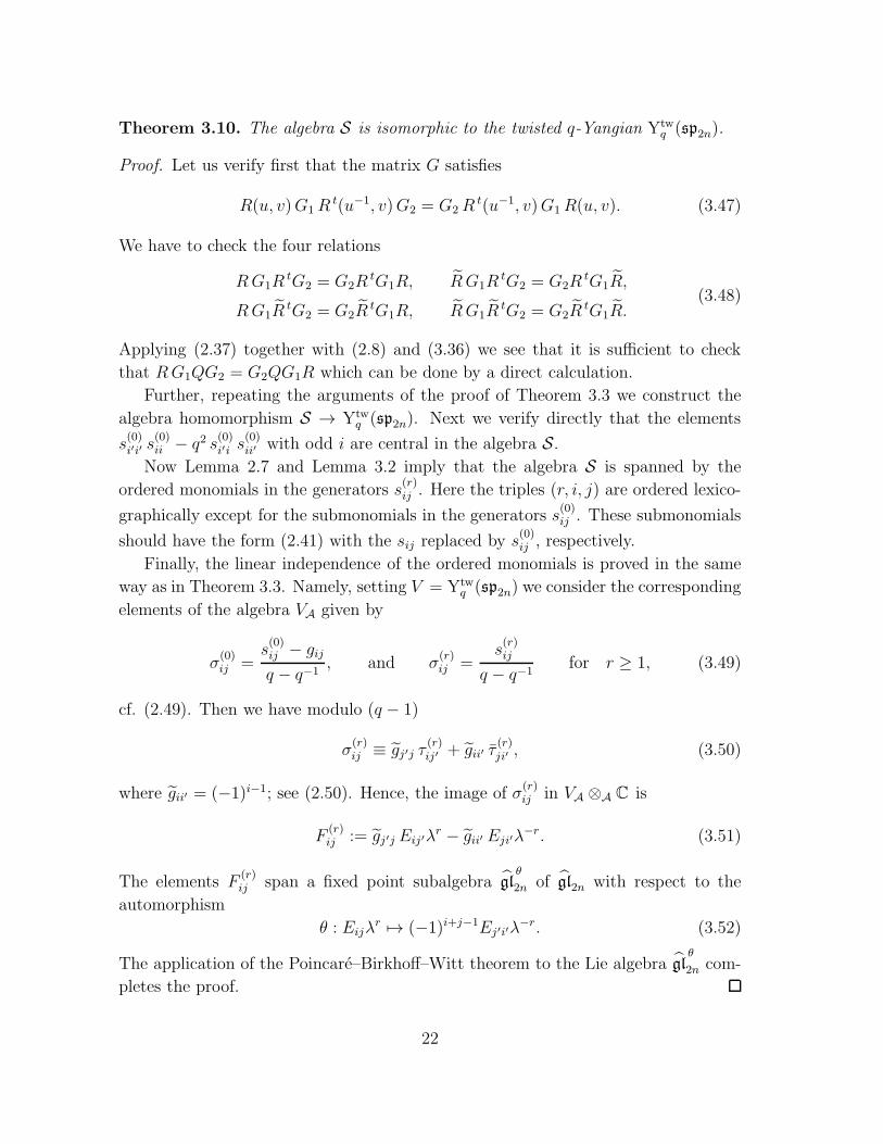
Theorem 3.10. The algebra S is isomorphic to the twisted q-Yangian Ytwq (sp2n).

Proof. Let us verify first that the matrix G satisfies

R(u, v)G1Rt(u−1, v)G2 = G2R

t(u−1, v)G1R(u, v). (3.47)

We have to check the four relations

RG1RtG2 = G2R

tG1R, RG1RtG2 = G2R

tG1R,

RG1RtG2 = G2R

tG1R, RG1RtG2 = G2R

tG1R.(3.48)

Applying (2.37) together with (2.8) and (3.36) we see that it is sufficient to check

that RG1QG2 = G2QG1R which can be done by a direct calculation.

Further, repeating the arguments of the proof of Theorem 3.3 we construct the

algebra homomorphism S → Ytwq (sp2n). Next we verify directly that the elements

s(0)i′i′ s

(0)ii − q2 s

(0)i′i s

(0)ii′ with odd i are central in the algebra S.

Now Lemma 2.7 and Lemma 3.2 imply that the algebra S is spanned by the

ordered monomials in the generators s(r)ij . Here the triples (r, i, j) are ordered lexico-

graphically except for the submonomials in the generators s(0)ij . These submonomials

should have the form (2.41) with the sij replaced by s(0)ij , respectively.

Finally, the linear independence of the ordered monomials is proved in the same

way as in Theorem 3.3. Namely, setting V = Ytwq (sp2n) we consider the corresponding

elements of the algebra VA given by

σ(0)ij =

s(0)ij − gij

q − q−1, and σ

(r)ij =

s(r)ij

q − q−1for r ≥ 1, (3.49)

cf. (2.49). Then we have modulo (q − 1)

σ(r)ij ≡ gj′j τ

(r)ij′ + gii′ τ

(r)ji′ , (3.50)

where gii′ = (−1)i−1; see (2.50). Hence, the image of σ(r)ij in VA ⊗A C is

F(r)ij := gj′j Eij′λ

r − gii′ Eji′λ−r. (3.51)

The elements F(r)ij span a fixed point subalgebra gl

θ

2n of gl2n with respect to the

automorphism

θ : Eijλr 7→ (−1)i+j−1Ej′i′λ

−r. (3.52)

The application of the Poincare–Birkhoff–Witt theorem to the Lie algebra glθ

2n com-

pletes the proof.

22

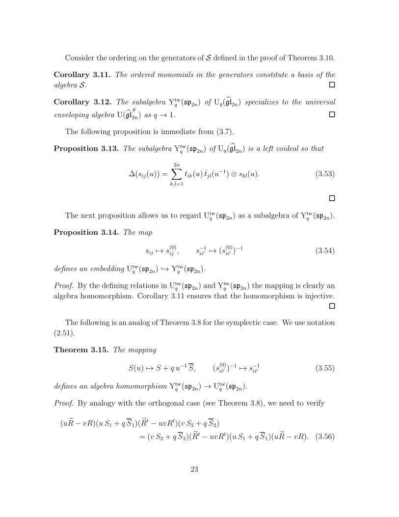
Consider the ordering on the generators of S defined in the proof of Theorem 3.10.

Corollary 3.11. The ordered monomials in the generators constitute a basis of the

algebra S.

Corollary 3.12. The subalgebra Ytwq (sp2n) of Uq(gl2n) specializes to the universal

enveloping algebra U(glθ

2n) as q → 1.

The following proposition is immediate from (3.7).

Proposition 3.13. The subalgebra Ytwq (sp2n) of Uq(gl2n) is a left coideal so that

∆(sij(u)) =2n∑

k,l=1

tik(u) tjl(u−1)⊗ skl(u). (3.53)

The next proposition allows us to regard Utwq (sp2n) as a subalgebra of Ytw

q (sp2n).

Proposition 3.14. The map

sij 7→ s(0)ij , s−1

ii′ 7→ (s(0)ii′ )

−1 (3.54)

defines an embedding Utwq (sp2n) → Ytw

q (sp2n).

Proof. By the defining relations in Utwq (sp2n) and Ytw

q (sp2n) the mapping is clearly an

algebra homomorphism. Corollary 3.11 ensures that the homomorphism is injective.

The following is an analog of Theorem 3.8 for the symplectic case. We use notation

(2.51).

Theorem 3.15. The mapping

S(u) 7→ S + q u−1 S, (s(0)ii′ )

−1 7→ s−1ii′ (3.55)

defines an algebra homomorphism Ytwq (sp2n) → Utw

q (sp2n).

Proof. By analogy with the orthogonal case (see Theorem 3.8), we need to verify

(uR− vR)(u S1 + q S1)(Rt − uvRt)(v S2 + q S2)

= (v S2 + q S2)(Rt − uvRt)(u S1 + q S1)(uR− vR). (3.56)

23

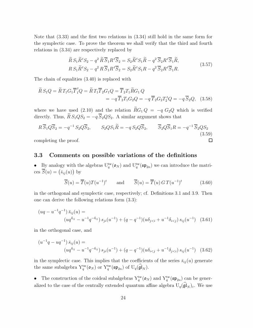
Note that (3.33) and the first two relations in (3.34) still hold in the same form for

the symplectic case. To prove the theorem we shall verify that the third and fourth

relations in (3.34) are respectively replaced by

R S1RtS2 − q2 R S1R

tS2 = S2RtS1R− q2 S2R

tS1R,

R S1RtS2 − q2RS1R

tS2 = S2RtS1R− q2 S2R

tS1R.(3.57)

The chain of equalities (3.40) is replaced with

R S1Q = R T1G1Tt

1Q = R T1T 2G1Q = T 2T1RG1Q

= −q T 2T1G2Q = −q T 2G2Tt2Q = −q S2Q, (3.58)

where we have used (2.10) and the relation RG1Q = −q G2Q which is verified

directly. Thus, R S1QS2 = −q S2QS2. A similar argument shows that

RS1QS2 = −q−1 S2QS2, S2QS1R = −q S2QS2, S2QS1R = −q−1 S2QS2

(3.59)

completing the proof.

3.3 Comments on possible variations of the definitions

• By analogy with the algebras Utwq (oN) and Utw

q (sp2n) we can introduce the matri-

ces S(u) =(sij(u)

)by

S(u) = T (u)T (u−1)t and S(u) = T (u)GT (u−1)t (3.60)

in the orthogonal and symplectic case, respectively; cf. Definitions 3.1 and 3.9. Then

one can derive the following relations form (3.3):

(uq − u−1q−1) sij(u) =

(uqδij − u−1q−δij ) sji(u−1) + (q − q−1)(uδj<i + u−1δi<j) sij(u

−1) (3.61)

in the orthogonal case, and

(u−1q − uq−1) sij(u) =

(uqδij − u−1q−δij ) sji(u−1) + (q − q−1)(uδi<j + u−1δj<i) sij(u

−1) (3.62)

in the symplectic case. This implies that the coefficients of the series sij(u) generate

the same subalgebra Ytwq (oN) or Y

twq (sp2n) of Uq(glN ).

• The construction of the coideal subalgebras Ytwq (oN) and Ytw

q (sp2n) can be gener-

alized to the case of the centrally extended quantum affine algebra Uq(glN )c. We use

24

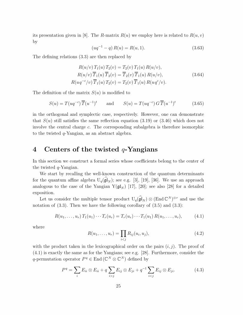
its presentation given in [8]. The R-matrix R(u) we employ here is related to R(u, v)

by

(uq−1 − q)R(u) = R(u, 1). (3.63)

The defining relations (3.3) are then replaced by

R(u/v) T1(u) T2(v) = T2(v) T1(u)R(u/v),

R(u/v) T 1(u) T 2(v) = T 2(v) T 1(u)R(u/v),

R(uq−c/v) T 1(u) T2(v) = T2(v) T 1(u)R(uqc/v).

(3.64)

The definition of the matrix S(u) is modified to

S(u) = T (uq−c) T (u−1)t and S(u) = T (uq−c)GT (u−1)t (3.65)

in the orthogonal and symplectic case, respectively. However, one can demonstrate

that S(u) still satisfies the same reflection equation (3.19) or (3.46) which does not

involve the central charge c. The corresponding subalgebra is therefore isomorphic

to the twisted q-Yangian, as an abstract algebra.

4 Centers of the twisted q-Yangians

In this section we construct a formal series whose coefficients belong to the center of

the twisted q-Yangian.

We start by recalling the well-known construction of the quantum determinants

for the quantum affine algebra Uq(glN); see e.g. [3], [19], [36]. We use an approach

analogous to the case of the Yangian Y(glN ) [17], [20]; see also [28] for a detailed

exposition.

Let us consider the multiple tensor product Uq(glN) ⊗ (EndCN )⊗r and use the

notation of (3.3). Then we have the following corollary of (3.5) and (3.3):

R(u1, . . . , ur) T1(u1) · · ·Tr(ur) = Tr(ur) · · ·T1(u1)R(u1, . . . , ur), (4.1)

where

R(u1, . . . , ur) =∏

i<j

Rij(ui, uj), (4.2)

with the product taken in the lexicographical order on the pairs (i, j). The proof of

(4.1) is exactly the same as for the Yangians; see e.g. [28]. Furthermore, consider the

q-permutation operator P q ∈ End (CN ⊗ CN) defined by

P q =∑

i

Eii ⊗Eii + q∑

i>j

Eij ⊗ Eji + q−1∑

i<j

Eij ⊗Eji. (4.3)

25

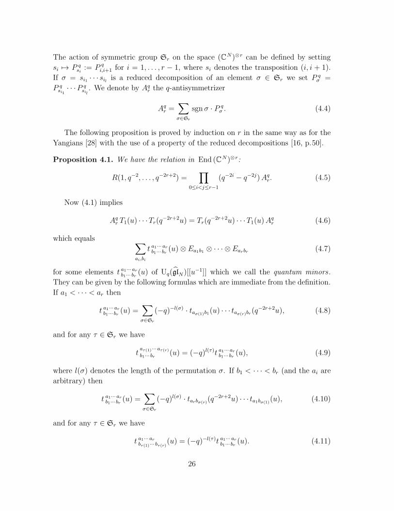
The action of symmetric group Sr on the space (CN)⊗r can be defined by setting

si 7→ P qsi:= P q

i,i+1 for i = 1, . . . , r − 1, where si denotes the transposition (i, i + 1).

If σ = si1 · · · sil is a reduced decomposition of an element σ ∈ Sr we set P qσ =

P qsi1

· · ·P qsil. We denote by Aq

r the q-antisymmetrizer

Aqr =

∑

σ∈Sr

sgn σ · P qσ . (4.4)

The following proposition is proved by induction on r in the same way as for the

Yangians [28] with the use of a property of the reduced decompositions [16, p.50].

Proposition 4.1. We have the relation in End (CN )⊗r:

R(1, q−2, . . . , q−2r+2) =∏

0≤i<j≤r−1

(q−2i − q−2j)Aqr. (4.5)

Now (4.1) implies

Aqr T1(u) · · ·Tr(q

−2r+2u) = Tr(q−2r+2u) · · ·T1(u)A

qr (4.6)

which equals ∑

ai,bi

t a1··· arb1··· br(u)⊗Ea1b1 ⊗ · · · ⊗Earbr (4.7)

for some elements t a1···arb1··· br(u) of Uq(glN)[[u

−1]] which we call the quantum minors .

They can be given by the following formulas which are immediate from the definition.

If a1 < · · · < ar then

t a1··· arb1··· br(u) =

∑

σ∈Sr

(−q)−l(σ) · taσ(1)b1(u) · · · taσ(r)br(q−2r+2u), (4.8)

and for any τ ∈ Sr we have

taτ(1)···aτ(r)b1··· br

(u) = (−q)l(τ)t a1··· arb1··· br(u), (4.9)

where l(σ) denotes the length of the permutation σ. If b1 < · · · < br (and the ai are

arbitrary) then

t a1··· arb1··· br(u) =

∑

σ∈Sr

(−q)l(σ) · tarbσ(r)(q−2r+2u) · · · ta1bσ(1)

(u), (4.10)

and for any τ ∈ Sr we have

t a1··· arbτ(1)··· bτ(r)(u) = (−q)−l(τ)t a1··· arb1··· br

(u). (4.11)

26

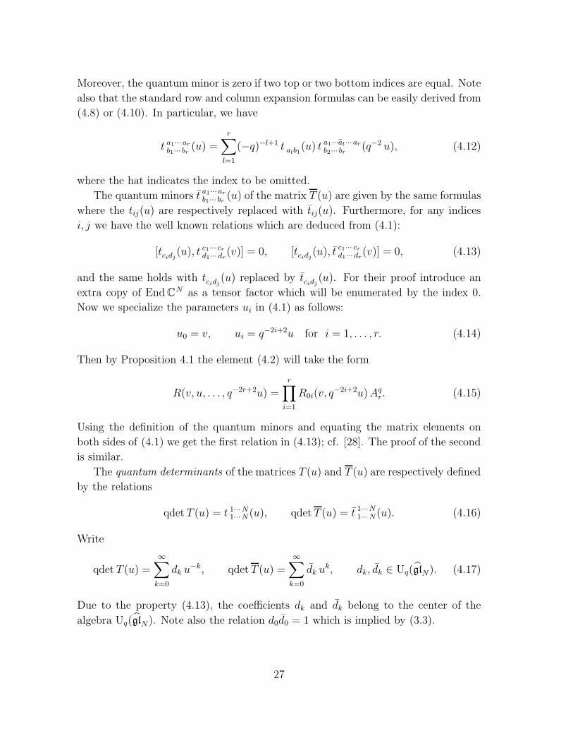
Moreover, the quantum minor is zero if two top or two bottom indices are equal. Note

also that the standard row and column expansion formulas can be easily derived from

(4.8) or (4.10). In particular, we have

t a1···arb1··· br(u) =

r∑

l=1

(−q)−l+1 t alb1(u) ta1···al···arb2··· br

(q−2 u), (4.12)

where the hat indicates the index to be omitted.

The quantum minors t a1···arb1··· br(u) of the matrix T (u) are given by the same formulas

where the tij(u) are respectively replaced with tij(u). Furthermore, for any indices

i, j we have the well known relations which are deduced from (4.1):

[tcidj (u), tc1··· crd1··· dr

(v)] = 0, [tcidj (u), tc1··· crd1··· dr

(v)] = 0, (4.13)

and the same holds with tcidj (u) replaced by tcidj (u). For their proof introduce an

extra copy of EndCN as a tensor factor which will be enumerated by the index 0.

Now we specialize the parameters ui in (4.1) as follows:

u0 = v, ui = q−2i+2u for i = 1, . . . , r. (4.14)

Then by Proposition 4.1 the element (4.2) will take the form

R(v, u, . . . , q−2r+2u) =r∏

i=1

R0i(v, q−2i+2u)Aq

r. (4.15)

Using the definition of the quantum minors and equating the matrix elements on

both sides of (4.1) we get the first relation in (4.13); cf. [28]. The proof of the second

is similar.

The quantum determinants of the matrices T (u) and T (u) are respectively defined

by the relations

qdet T (u) = t 1···N1···N(u), qdet T (u) = t 1···N1···N(u). (4.16)

Write

qdet T (u) =∞∑

k=0

dk u−k, qdet T (u) =

∞∑

k=0

dk uk, dk, dk ∈ Uq(glN). (4.17)

Due to the property (4.13), the coefficients dk and dk belong to the center of the

algebra Uq(glN). Note also the relation d0d0 = 1 which is implied by (3.3).

27

4.1 Sklyanin determinant

We shall consider the orthogonal and symplectic cases simultaneously unless otherwise

stated. The symbol Ytwq will denote either Ytw

q (oN) or Ytwq (spN) (the latter with

N = 2n). As before, we denote by S(u) the matrix T (u)GT (u−1)t, where G is the

identity matrix in the orthogonal case, and G is given by (2.33) in the symplectic case.

Then S(u) satisfies the relations (3.19) and (3.46), respectively, which have the same

form. Our arguments are similar to those used in [35] and [28] for the construction

of the Sklyanin determinant for the twisted Yangians.

The following relation in the algebra Ytwq ⊗ (EndCN)⊗r is a corollary of (3.46).

R(u1, . . . , ur)S1(u1)Rt12 · · ·R

t1rS2(u2)R

t23 · · ·R

t2rS3(u3) · · ·R

tr−1,rSr(ur) =

Sr(ur)Rtr−1,r · · ·S3(u3)R

t2r · · ·R

t23S2(u2)R

t1r · · ·R

t12S1(u1)R(u1, . . . , ur), (4.18)

where R(u1, . . . , ur) is given by (4.2) and R tij = R t

ij(u−1i , uj). Now take r = N and

specify ui = u q−2i+2. Then Proposition 4.1 implies

AqN S1(u)R

t12 · · ·R

t1NS2(u q

−2)R t23 · · ·R

t2NS3(u q

−4) · · ·R tN−1,NSN(u q

−2N+2) =

SN (u q−2N+2)R t

N−1,N · · ·S3(u q−4)R t

2N · · ·R t23S2(u q

−2)R t1N · · ·R t

12S1(u)AqN . (4.19)

Since the q-antisymmetrizer AqN is proportional to an idempotent and maps the space

(CN)⊗N into a one-dimensional subspace, both sides must be equal to AqN times a

series sdet S(u) in u−1 with coefficients in Ytwq . We call this series the Sklyanin

determinant .

The following theorem provides an expression of sdetS(u) in terms of the quantum

determinants.

Theorem 4.2. We have

sdet S(u) = γN(u) qdet T (u) qdetT (q2N−2u−1), (4.20)

where

γN(u) =∏

1≤i<j≤N

(q2i−2u−1 − q−2j+2u) ·

1 in the case of oN ,

qn−2 − qnu2

q2n−2 − q−2nu2in the case of sp2n.

(4.21)

Proof. We follow the arguments of [28, Section 4]. Substitute S(u) = T (u)GT (u−1)t

into (4.19) and transform the left hand side using the relations

T i(u−1)tRt

ij(u−1, v) Tj(v) = Tj(v)R

tij(u

−1, v) T i(u−1)t (4.22)

28

which are implied by (3.3). We then bring it to the form

AqN T1(u) · · ·TN (q

−2N+2u) R(u) T 1(u−1)t · · ·TN(q

2N−2u−1)t, (4.23)

where

R(u) = G1Rt12 · · ·R

t1NG2R

t23 · · ·R

t2NG3 · · ·R

tN−1,NGN . (4.24)

By the definition of the quantum determinant we have

AqN T1(u) · · ·TN(q

−2N+2u) = AqN qdet T (u). (4.25)

Further, using the homomorphism S(u) 7→ G we derive from (4.19)

AqNR(u) = GNR

tN−1,N · · ·G3R

t2N · · ·R t

23G2Rt1N · · ·R t

12G1AqN . (4.26)

Thus, this expression equals AqNγN(u) for a scalar function γN(u). Using the explicit

formulas (4.8) one easily derives that

AqN T 1(u

−1)t · · ·TN(q2N−2u−1)t = Aq

N qdet T (q2N−2u−1). (4.27)

It remains to calculate the function γN(u). Consider first the orthogonal case. Apply

the operator AqNR(u) to the basis vector e1 ⊗ · · · ⊗ eN , where the ei denote the

canonical basis vectors of CN . By (3.16) the result is clearly γN(u)AqN(e1⊗· · ·⊗ eN )

with γN(u) given by (4.21). In the symplectic case apply Aq2nR(u) to the basis vector

v = e2n−1 ⊗ e2n−3 ⊗ · · · ⊗ e1 ⊗ e2 ⊗ e4 ⊗ · · · ⊗ e2n. (4.28)

Since Ge2k = q e2k−1 the vector Aq2nR(u) v equals

qn∏

n≤i<j≤2n

(q2i−2u−1−q−2j+2u)Aq2nG1R

t12 · · ·R

t1,2nG2 · · ·GnR

tn,n+1 · · ·R

tn,2n w, (4.29)

where

w = e2n−1 ⊗ e2n−3 ⊗ · · · ⊗ e1 ⊗ e1 ⊗ e3 ⊗ · · · ⊗ e2n−1. (4.30)

If j > n+ 1 then R tn,j w = (q2n−2u−1 − q−2j+2u)w. Further, we have

R tn,n+1 (e1⊗e1) = (q2n−3u−1−q−2n+1u) (e1⊗e1)+(q−1−q) q−2n u

2n∑

k=2

(ek⊗ek). (4.31)

Next apply the operator Gn and note that due to the subsequent application of the

q-antisymmetrizer, we may only keep the linear combination of the tensor products

29

containing e1 or e2 on the n-th and (n+1)-th places (see [28, Section 4] for a similar

argument in the symplectic twisted Yangian case). That is, we may write

Aq2nG1R

t12 · · ·R

t1,2nG2 · · ·GnR

tn,n+1w =

(q2n−4u−1 − q−2n+2u)Aq2nG1R

t12 · · ·R

t1,2nG2 · · ·Gn−1R

tn−1,n · · ·R

tn−1,2n w

′ (4.32)

with

w′ = e2n−1 ⊗ e2n−3 ⊗ · · · ⊗ e3 ⊗ e1 ⊗ e2 ⊗ e3 ⊗ · · · ⊗ e2n−1. (4.33)

By the skew-symmetry of the antisymmetrizer replace w′ with the vector

w′′ = e2n−1 ⊗ e2n−3 ⊗ · · · ⊗ e3 ⊗ e3 ⊗ e2 ⊗ e1 ⊗ · · · ⊗ e2n−1, (4.34)

taking the sign into account. Continuing the calculation in a similar manner, we

conclude that the product of the scalar factors occurring in the procedure will coincide

with γ2n(u) given in (4.21) with N = 2n.

The centrality of qdet T (u) and qdet T (u) in Uq(glN) immediately implies the

corresponding property of the Sklyanin determinant sdet S(u).

Corollary 4.3. The coefficients of the series sdet S(u) belong to the center of the

algebra Ytwq .

Introduce the series c(u) and the elements ck of the center of the algebra Ytwq by

the formula

c(u) = γN(u)−1 sdetS(u) = 1 +

∞∑

k=1

ck u−k. (4.35)

The series begins with 1 due to Theorem 4.2 and the relation d0d0 = 1.

Proposition 4.4. The coefficients ck, k ≥ 1 are algebraically independent.

Proof. The coefficients {dk, k ≥ 0, dk, k ≥ 1} of the quantum determinants are

algebraically independent. This can be derived by analogy with the case of the

Yangian; see e.g. [28, Section 2]. The key observation here is the isomorphism (3.10).

The statement is now implied by Theorem 4.2.

Since both evaluation homomorphisms (3.31) and (3.55) are surjective, we obtain

families of central elements in the algebras Utwq (oN) and Utw

q (sp2n) as images of the

coefficients of sdetS(u). In other words, we have the following result.

Proposition 4.5. The coefficients of the Sklyanin determinants sdet (S + q−1u−1S)

and sdet (S + qu−1S) are central elements in the algebras Utwq (oN) and Utw

q (sp2n),

respectively.

30

In what follows we only consider the case of the orthogonal twisted q-Yangian

Ytwq (oN). In order to produce an explicit formula for the corresponding Sklyanin

determinant we introduce a map

πN : SN → SN , p 7→ p′ (4.36)

which was previously used in the ‘short’ formula for the Sklyanin determinant for the

twisted Yangians; see [27]. This map is defined by an inductive procedure. Given a set

of positive integers ω1 < · · · < ωN we regard SN as the group of their permutations.

If N = 2 we define π2 as the map S2 → S2 whose image is the identity permutation.

For N > 2 define a map from the set of ordered pairs (ωk, ωl) with k 6= l into itself

by the rule(ωk, ωl) 7→ (ωl, ωk), k, l < N,

(ωk, ωN) 7→ (ωN−1, ωk), k < N − 1,

(ωN , ωk) 7→ (ωk, ωN−1), k < N − 1,

(ωN−1, ωN) 7→ (ωN−1, ωN−2),

(ωN , ωN−1) 7→ (ωN−1, ωN−2).

(4.37)

Let p = (p1, . . . , pN) be a permutation of the indices ω1, . . . , ωN . Its image under the

map πN is the permutation p ′ = (p ′1, . . . , p

′N−1, ωN), where the pair (p ′

1, p′N−1) is the

image of the ordered pair (p1, pN) under the map (4.37). Then the pair (p ′2, p

′N−2)

is found as the image of (p2, pN−1) under the map (4.37) which is defined on the set

of ordered pairs of elements obtained from (ω1, . . . , ωN) by deleting p1 and pN ; etc.

The map πN has curious combinatorial properties which were observed by Lascoux;

see [26]. In particular, each fiber of this map is an interval in SN with respect to the

Bruhat order, isomorphic to a Boolean poset.

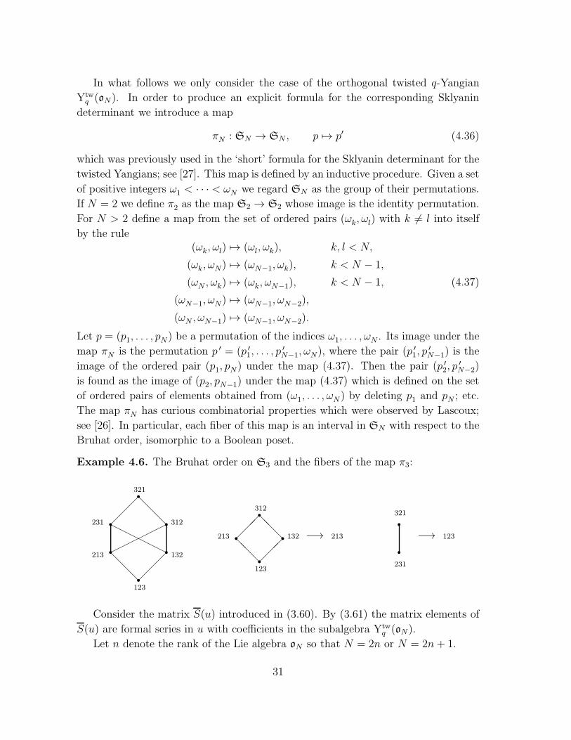
Example 4.6. The Bruhat order on S3 and the fibers of the map π3:

r

r r

r r

r

���

❅❅

❅

���

❅❅

❅

✟✟✟✟✟✟

❍❍❍❍❍❍

123

213 132

231 312

321

r

r

r r

���

❅❅❅���

❅❅❅

123

213

312

132 −→ 213

r

r

231

321

−→ 123

Consider the matrix S(u) introduced in (3.60). By (3.61) the matrix elements of

S(u) are formal series in u with coefficients in the subalgebra Ytwq (oN).

Let n denote the rank of the Lie algebra oN so that N = 2n or N = 2n + 1.

31

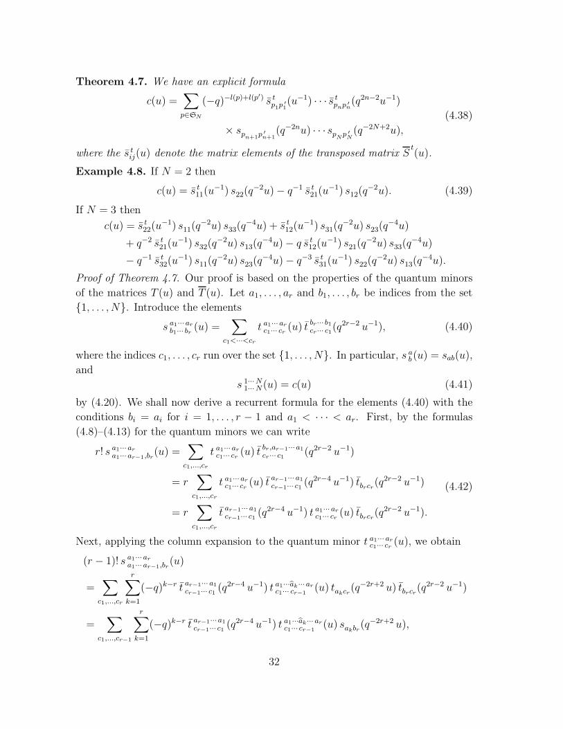
Theorem 4.7. We have an explicit formula

c(u) =∑

p∈SN

(−q)−l(p)+l(p′) s tp1p

′

1(u−1) · · · s t

pnp′

n(q2n−2u−1)

× spn+1p′

n+1(q−2nu) · · · sp

Np ′

N(q−2N+2u),

(4.38)

where the s tij(u) denote the matrix elements of the transposed matrix S

t(u).

Example 4.8. If N = 2 then

c(u) = s t11(u

−1) s22(q−2u)− q−1 s t

21(u−1) s12(q

−2u). (4.39)

If N = 3 then

c(u) = s t22(u

−1) s11(q−2u) s33(q

−4u) + s t12(u

−1) s31(q−2u) s23(q

−4u)

+ q−2 s t21(u

−1) s32(q−2u) s13(q

−4u)− q s t12(u

−1) s21(q−2u) s33(q

−4u)

− q−1 s t32(u

−1) s11(q−2u) s23(q

−4u)− q−3 s t31(u

−1) s22(q−2u) s13(q

−4u).

Proof of Theorem 4.7. Our proof is based on the properties of the quantum minors

of the matrices T (u) and T (u). Let a1, . . . , ar and b1, . . . , br be indices from the set

{1, . . . , N}. Introduce the elements

s a1··· arb1··· br

(u) =∑

c1<···<cr

t a1··· arc1··· cr(u) t br ··· b1cr··· c1

(q2r−2 u−1), (4.40)

where the indices c1, . . . , cr run over the set {1, . . . , N}. In particular, s ab (u) = sab(u),

and

s 1···N1···N(u) = c(u) (4.41)

by (4.20). We shall now derive a recurrent formula for the elements (4.40) with the

conditions bi = ai for i = 1, . . . , r − 1 and a1 < · · · < ar. First, by the formulas

(4.8)–(4.13) for the quantum minors we can write

r! s a1···ara1···ar−1,br

(u) =∑

c1,...,cr

t a1··· arc1··· cr(u) t br ,ar−1···a1

cr··· c1(q2r−2 u−1)

= r∑

c1,...,cr

t a1···arc1··· cr(u) t ar−1··· a1

cr−1··· c1(q2r−4 u−1) tbrcr(q

2r−2 u−1)

= r∑

c1,...,cr

t ar−1··· a1cr−1··· c1

(q2r−4 u−1) t a1··· arc1··· cr(u) tbrcr(q

2r−2 u−1).

(4.42)

Next, applying the column expansion to the quantum minor t a1··· arc1··· cr(u), we obtain

(r − 1)! s a1··· ara1··· ar−1,br

(u)

=∑

c1,...,cr

r∑

k=1

(−q)k−r t ar−1··· a1cr−1··· c1

(q2r−4 u−1) t a1···ak ···arc1··· cr−1(u) takcr(q

−2r+2 u) tbrcr(q2r−2 u−1)

=∑

c1,...,cr−1

r∑

k=1

(−q)k−r t ar−1···a1cr−1··· c1

(q2r−4 u−1) t a1···ak··· arc1··· cr−1(u) sakbr(q

−2r+2 u),

32

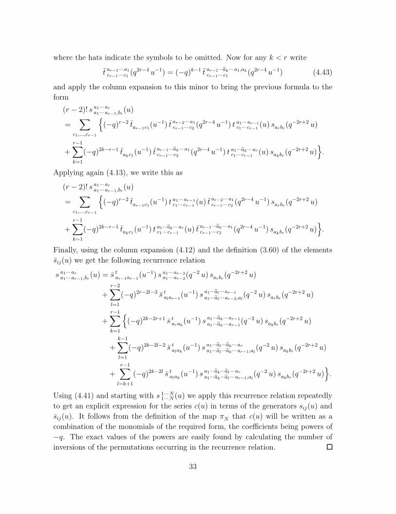
where the hats indicate the symbols to be omitted. Now for any k < r write

t ar−1···a1cr−1··· c1

(q2r−4 u−1) = (−q)k−1 t ar−1···ak ···a1,akcr−1··· c1

(q2r−4 u−1) (4.43)

and apply the column expansion to this minor to bring the previous formula to the

form

(r − 2)! s a1··· ara1··· ar−1,br

(u)

=∑

c1,...,cr−1

{(−q)r−2 tar−1c1

(u−1) t ar−2···a1cr−1··· c2

(q2r−4 u−1) t a1···ar−1c1··· cr−1

(u) sarbr(q−2r+2 u)

+r−1∑

k=1

(−q)2k−r−1 takc1(u−1) t ar−1···ak ···a1

cr−1··· c2(q2r−4 u−1) t a1···ak··· arc1··· cr−1

(u) sakbr(q−2r+2 u)

}.

Applying again (4.13), we write this as

(r − 2)! s a1··· ara1··· ar−1,br

(u)

=∑

c1,...,cr−1

{(−q)r−2 tar−1c1

(u−1) t a1··· ar−1c1··· cr−1

(u) t ar−2···a1cr−1··· c2

(q2r−4 u−1) sarbr(q−2r+2 u)

+

r−1∑

k=1

(−q)2k−r−1 takc1(u−1) t a1···ak··· arc1··· cr−1

(u) t ar−1···ak ··· a1cr−1··· c2

(q2r−4 u−1) sakbr(q−2r+2 u)

}.

Finally, using the column expansion (4.12) and the definition (3.60) of the elements

sij(u) we get the following recurrence relation

s a1···ara1···ar−1,br

(u) = s tar−1ar−1

(u−1) s a1···ar−2a1···ar−2

(q−2 u) sarbr(q−2r+2 u)

+r−2∑

l=1

(−q)2r−2l−3 s talar−1

(u−1) sa1···al···ar−1

a1···al···ar−2,al(q−2 u) sarbr(q

−2r+2 u)

+r−1∑

k=1

{(−q)2k−2r+1 s t

arak(u−1) s

a1···ak ···ar−1

a1···ak ···ar−1(q−2 u) sakbr(q

−2r+2 u)

+k−1∑

l=1

(−q)2k−2l−2 s talak

(u−1) s a1···al···ak··· ara1···al···ak··· ar−1,al

(q−2 u) sakbr(q−2r+2 u)

+r−1∑

l=k+1

(−q)2k−2l s talak

(u−1) s a1···ak···al···ara1···ak···al···ar−1,al

(q−2 u) sakbr(q−2r+2 u)

}.

Using (4.41) and starting with s 1···N1···N (u) we apply this recurrence relation repeatedly

to get an explicit expression for the series c(u) in terms of the generators sij(u) and

sij(u). It follows from the definition of the map πN that c(u) will be written as a

combination of the monomials of the required form, the coefficients being powers of

−q. The exact values of the powers are easily found by calculating the number of

inversions of the permutations occurring in the recurrence relation.

33

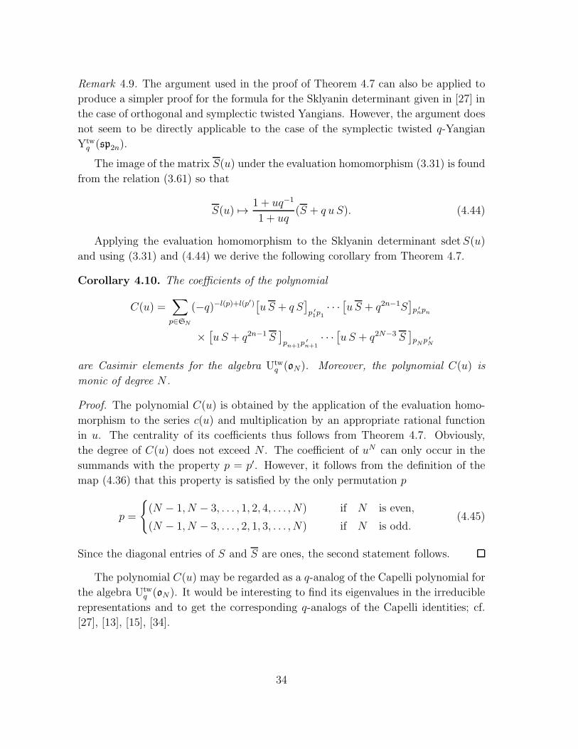
Remark 4.9. The argument used in the proof of Theorem 4.7 can also be applied to

produce a simpler proof for the formula for the Sklyanin determinant given in [27] in

the case of orthogonal and symplectic twisted Yangians. However, the argument does

not seem to be directly applicable to the case of the symplectic twisted q-Yangian

Ytwq (sp2n).

The image of the matrix S(u) under the evaluation homomorphism (3.31) is found

from the relation (3.61) so that

S(u) 7→1 + uq−1

1 + uq(S + q u S). (4.44)

Applying the evaluation homomorphism to the Sklyanin determinant sdetS(u)

and using (3.31) and (4.44) we derive the following corollary from Theorem 4.7.

Corollary 4.10. The coefficients of the polynomial

C(u) =∑

p∈SN

(−q)−l(p)+l(p′)[u S + q S

]p ′

1p1· · ·

[u S + q2n−1S

]p ′

npn

×[u S + q2n−1 S

]pn+1p

′

n+1· · ·

[u S + q2N−3 S

]pNp ′

N

are Casimir elements for the algebra Utwq (oN). Moreover, the polynomial C(u) is

monic of degree N .

Proof. The polynomial C(u) is obtained by the application of the evaluation homo-

morphism to the series c(u) and multiplication by an appropriate rational function

in u. The centrality of its coefficients thus follows from Theorem 4.7. Obviously,

the degree of C(u) does not exceed N . The coefficient of uN can only occur in the

summands with the property p = p′. However, it follows from the definition of the

map (4.36) that this property is satisfied by the only permutation p

p =

{(N − 1, N − 3, . . . , 1, 2, 4, . . . , N) if N is even,

(N − 1, N − 3, . . . , 2, 1, 3, . . . , N) if N is odd.(4.45)

Since the diagonal entries of S and S are ones, the second statement follows.

The polynomial C(u) may be regarded as a q-analog of the Capelli polynomial for

the algebra Utwq (oN). It would be interesting to find its eigenvalues in the irreducible

representations and to get the corresponding q-analogs of the Capelli identities; cf.

[27], [13], [15], [34].

34

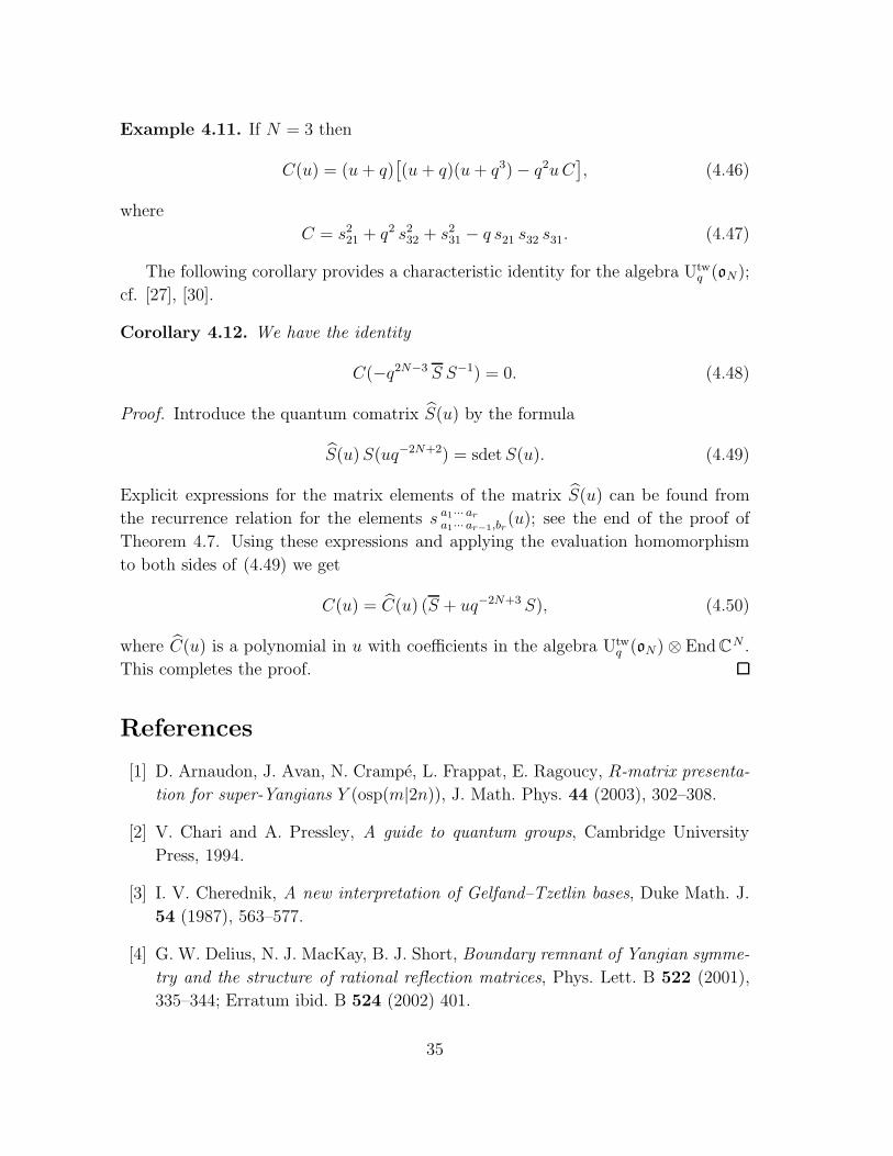
Example 4.11. If N = 3 then

C(u) = (u+ q)[(u+ q)(u+ q3)− q2uC

], (4.46)

where

C = s221 + q2 s232 + s231 − q s21 s32 s31. (4.47)

The following corollary provides a characteristic identity for the algebra Utwq (oN);

cf. [27], [30].

Corollary 4.12. We have the identity

C(−q2N−3 S S−1) = 0. (4.48)

Proof. Introduce the quantum comatrix S(u) by the formula

S(u)S(uq−2N+2) = sdet S(u). (4.49)

Explicit expressions for the matrix elements of the matrix S(u) can be found from

the recurrence relation for the elements s a1··· ara1··· ar−1,br

(u); see the end of the proof of

Theorem 4.7. Using these expressions and applying the evaluation homomorphism

to both sides of (4.49) we get

C(u) = C(u) (S + uq−2N+3 S), (4.50)

where C(u) is a polynomial in u with coefficients in the algebra Utwq (oN)⊗ EndCN .

This completes the proof.

References

[1] D. Arnaudon, J. Avan, N. Crampe, L. Frappat, E. Ragoucy, R-matrix presenta-

tion for super-Yangians Y (osp(m|2n)), J. Math. Phys. 44 (2003), 302–308.

[2] V. Chari and A. Pressley, A guide to quantum groups, Cambridge University

Press, 1994.

[3] I. V. Cherednik, A new interpretation of Gelfand–Tzetlin bases, Duke Math. J.

54 (1987), 563–577.

[4] G. W. Delius, N. J. MacKay, B. J. Short, Boundary remnant of Yangian symme-

try and the structure of rational reflection matrices, Phys. Lett. B 522 (2001),

335–344; Erratum ibid. B 524 (2002) 401.

35

[5] G. W. Delius and N. J. MacKay, Quantum group symmetry in sine-Gordon and

affine Toda field theories on the half-line, Comm. Math. Phys. 233 (2003), 173–

190.

[6] M. S. Dijkhuizen and M. Noumi, A family of quantum projective spaces and

related q-hypergeometric orthogonal polynomials, Trans. AMS 350 (1998), 3269–

3296.

[7] M. S. Dijkhuizen, M. Noumi and T. Sugitani, Multivariable Askey–Wilson poly-

nomials and quantum complex Grassmannians, Fields Int. Commun. 14 (1997),

167–177.

[8] J. Ding, Spinor representations of Uq(gl(n)) and quantum boson-fermion corre-

spondence, Comm. Math. Phys. 200 (1999), 399–420.

[9] V. G. Drinfeld, Hopf algebras and the quantum Yang–Baxter equation, Soviet

Math. Dokl. 32 (1985), 254–258.

[10] V. G. Drinfeld, A new realization of Yangians and quantized affine algebras,

Soviet Math. Dokl. 36 (1988), 212–216.

[11] E. Frenkel and E. Mukhin, The Hopf algebra RepUqgl∞, Selecta Math. (N.S.) 8

(2002), 537–635.

[12] A. M. Gavrilik and A. U. Klimyk, q-deformed orthogonal and pseudo-orthogonal

algebras and their representations, Lett. Math. Phys. 21 (1991), 215–220.

[13] A. M. Gavrilik and N. Z. Iorgov, On Casimir elements of q-algebras U ′q(son) and

their eigenvalues in representations, in ‘Symmetry in nonlinear mathematical

physics’, Proc. Inst. Mat. Ukr. Nat. Acad. Sci. 30, Kyiv, 1999, pp. 310–314.

[14] A. M. Gavrilik, N. Z. Iorgov and A. U. Klimyk, Nonstandard deformation

U ′q(son): the embedding U ′

q(son) ⊂ Uq(sln) and representations, in ‘Symmetries

in science’, X (Bregenz, 1997). Plenum, New-York, 1998, pp. 121–133.

[15] M. Havlıcek, A. U. Klimyk and S. Posta, Central elements of the algebras U ′q(som)

and Uq(isom), Czechoslovak J. Phys. 50 (2000), 79–84.

[16] J. E. Humphreys, Introduction to Lie algebras and Representation Theory,

Springer, New York, 1972.

[17] A. G. Izergin and V. E. Korepin, A lattice model related to the nonlinear

Schrodinger equation, Sov. Phys. Dokl. 26 (1981) 653–654.

36

[18] M. Jimbo, A q-difference analogue of U(g) and the Yang–Baxter equation, Lett.

Math. Phys. 10 (1985), 63–69.

[19] M. Jimbo, A q-analogue of Uq(gl(N + 1)), Hecke algebra and the Yang–Baxter

equation, Lett. Math. Phys. 11 (1986), 247–252.

[20] P. P. Kulish and E. K. Sklyanin, Quantum spectral transform method: recent

developments, in ‘Integrable Quantum Field Theories’, Lecture Notes in Phys.

151 Springer, Berlin-Heidelberg, 1982, pp. 61–119.

[21] G. Letzter, Symmetric pairs for quantized enveloping algebras, J. Algebra 220

(1999), 729–767.

[22] G. Letzter, Coideal subalgebras and quantum symmetric pairs, in ‘New direc-

tions in Hopf algebras’, Math. Sci. Res. Inst. Publ. 43, Cambridge Univ. Press,

Cambridge, 2002, pp. 117–165.

[23] G. Letzter, Quantum symmetric pairs and their zonal spherical functions,

preprint math.QA/0204103.

[24] A. Liguori, M. Mintchev and L. Zhao, Boundary exchange algebras and scattering

on the half line, Comm. Math. Phys. 194 (1998), 569–589.

[25] M. Mintchev, E. Ragoucy and P. Sorba, Spontaneous symmetry breaking in the

gl(N)-NLS hierarchy on the half line, J. Phys. A 34 (2001), 8345–8364.

[26] A. I. Molev, Stirling partitions of the symmetric group and Laplace operators for

the orthogonal Lie algebra, Discrete Math. 180 (1998), 281–300.

[27] A. I. Molev, Yangians and their applications, in “Handbook of Algebra”, Vol. 3,

(M. Hazewinkel, Ed.), Elsevier, 2003.

[28] A. Molev, M. Nazarov and G. Olshanski, Yangians and classical Lie algebras,

Russian Math. Surveys 51:2 (1996), 205–282.

[29] A. I. Molev and E. Ragoucy, Representations of reflection algebras, Rev. Math.

Phys. 14 (2002), 317–342.

[30] M. Nazarov and V. Tarasov, Yangians and Gelfand–Zetlin bases, Publ. RIMS,

Kyoto Univ. 30 (1994), 459–478.

[31] M. Noumi, Macdonald’s symmetric polynomials as zonal spherical functions on

quantum homogeneous spaces, Adv. Math. 123 (1996), 16–77.

37

[32] M. Noumi and T. Sugitani, Quantum symmetric spaces and related q-orthogonal

polynomials, in ‘Group Theoretical Methods in Physics (ICGTMP)’ (Toyonaka,

Japan, 1994), World Sci. Publishing, River Edge, N.J. (1995), pp. 28–40.

[33] M. Noumi, T. Umeda and M. Wakayama, A quantum dual pair (sl2, on) and the

associated Capelli identity, Lett. Math. Phys. 34 (1995), 1–8.

[34] M. Noumi, T. Umeda and M. Wakayama, Dual pairs, spherical harmonics and a

Capelli identity in quantum group theory, Compos. Math. 104 (1996), 227–277.

[35] G. Olshanski, Twisted Yangians and infinite-dimensional classical Lie algebras,

in ‘Quantum Groups’ (P. P. Kulish, Ed.), Lecture Notes in Math. 1510, Springer,

Berlin-Heidelberg, 1992, pp. 103–120.

[36] N. Yu. Reshetikhin, L. A. Takhtajan and L. D. Faddeev, Quantization of Lie

Groups and Lie algebras, Leningrad Math. J. 1 (1990), 193–225.

[37] E. K. Sklyanin, Boundary conditions for integrable quantum systems, J. Phys.

A21 (1988), 2375–2389.

38