1

Coarse grained modeling: applications in polymers and biological systems

Presented byYongmei Wang

Department of ChemistryThe University of MemphisMemphis, Tennessee 38152

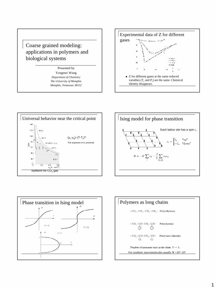
Experimental data of Z for different gases

n Z for different gases at the same reduced variables (Tr and Pr) are the same. Chemical identity disappears.

Universal behavior near the critical point

(ρL-ρg)~(T-Tc)m

The exponent m is universal

Isotherm for CO2 gas

Ising model for phase transition

Each lattice site has a spin σi

Phase transition in Ising model Polymers as long chains

For synthetic macromolecules usually N =102~104

2

solid45066C30H62triacontane

34337C20H42eicosane

216-10C12H26dodecane

196-25C11H24undecane

174-30C10H22decane

liquid151-51C9H20nonane

125-57C8H18octane

98-91C7H16heptane

69-95C6H14hexane

36-130C5H12pentane

-0.5-138C4H10butane

-42.8-190C3H8propane

-89-183C2H6ethane

gas-164-183CH4methane

State at25oC

BoilingPoint (oC)

MeltingPoint (oC)

MolecularFormula

Name

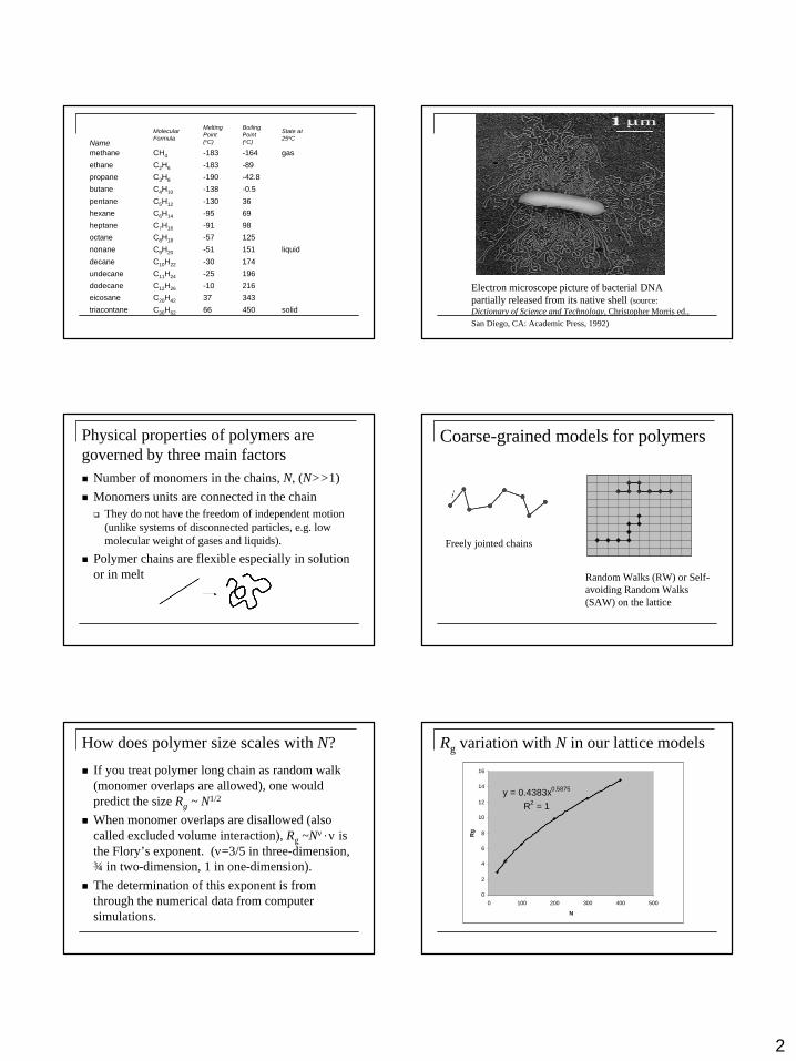
Electron microscope picture of bacterial DNA partially released from its native shell (source: Dictionary of Science and Technology, Christopher Morris ed., San Diego, CA: Academic Press, 1992)

Physical properties of polymers are governed by three main factorsn Number of monomers in the chains, N, (N>>1)n Monomers units are connected in the chainq They do not have the freedom of independent motion

(unlike systems of disconnected particles, e.g. low molecular weight of gases and liquids).

n Polymer chains are flexible especially in solution or in melt

Coarse-grained models for polymers

Freely jointed chains

Random Walks (RW) or Self-avoiding Random Walks (SAW) on the lattice

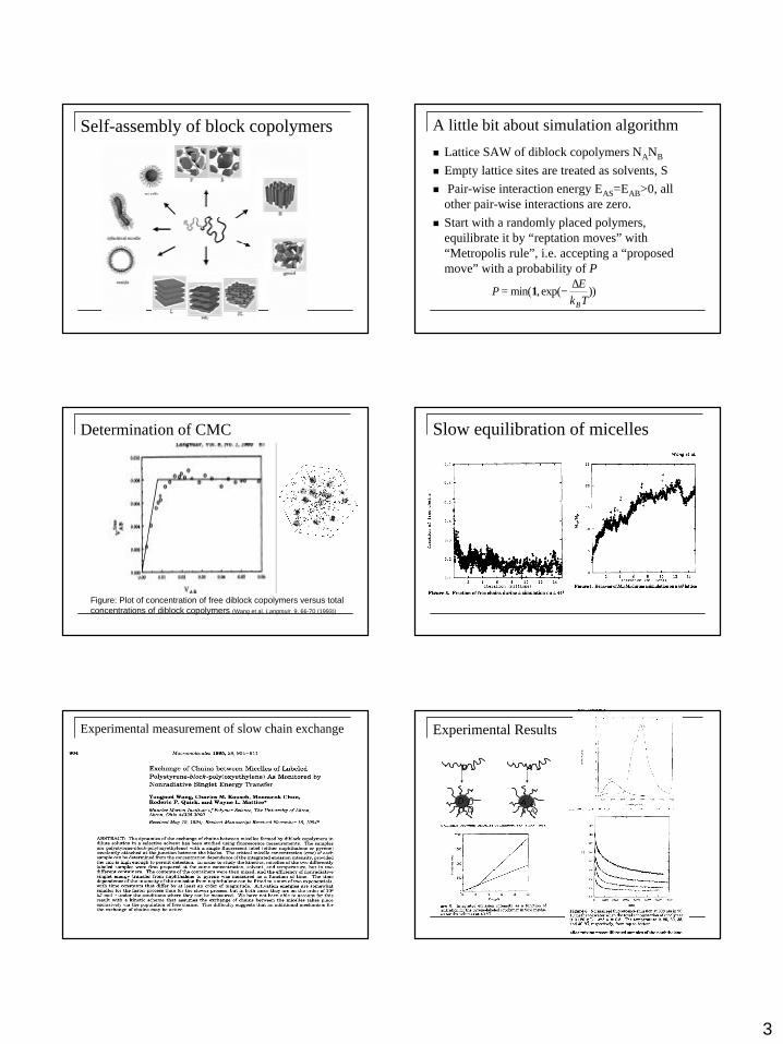
How does polymer size scales with N?

n If you treat polymer long chain as random walk (monomer overlaps are allowed), one would predict the size Rg ~ N1/2

n When monomer overlaps are disallowed (also called excluded volume interaction), Rg ~Nν , ν is the Flory’s exponent. (ν=3/5 in three-dimension, ¾ in two-dimension, 1 in one-dimension).

n The determination of this exponent is from through the numerical data from computer simulations.

Rg variation with N in our lattice models

y = 0.4383x0.5875

R2 = 1

0

2

4

6

8

10

12

14

16

0 100 200 300 400 500

N

Rg

3

Self-assembly of block copolymers A little bit about simulation algorithm

n Lattice SAW of diblock copolymers NANB

n Empty lattice sites are treated as solvents, Sn Pair-wise interaction energy EAS=EAB>0, all

other pair-wise interactions are zero.n Start with a randomly placed polymers,

equilibrate it by “reptation moves” with “Metropolis rule”, i.e. accepting a “proposed move” with a probability of P

PE

k TB

= −min( , exp( ))1∆

Figure: Plot of concentration of free diblock copolymers versus total concentrations of diblock copolymers (Wang et al, Langmuir, 9, 66-70 (1993))

Determination of CMC Slow equilibration of micelles

Experimental measurement of slow chain exchange Experimental Results

D A

DDDD

AAAA

4

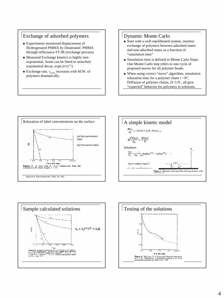
Exchange of adsorbed polymersn Experiments monitored displacement of

Hydrogenated PMMA by Deuterated PMMA through reflectance FT-IR (exchange process)

n Measured Exchange kinetics is highly non-exponential. Some can be fitted to stretched-exponential decay, exp(-(t/τ)1/2)

n Exchange rate, τexch increases with M.W. of polymers dramatically.

Dynamic Monte Carlo n Start with a well-equilibrated system, monitor

exchange of polymers between adsorbed states and non-adsorbed states as a function of “simulation time”

n Simulation time is defined in Monte Carlo Steps. One Monte Carlo step refers to one cycle of proposed moves for all polymer beads.

n When using correct “move” algorithm, simulation relaxation time for a polymer chain τ ~N2, Diffusion of polymer chains, D~1/N , all give “expected” behavior for polymers in solutions.

Relaxation of label concentrations on the surface

Wang et al, Macromolecules, 1995, 28, 7061

(a) Non-permanent label

(b) Permanent label

A simple kinetic model

Solutions:

Sample calculated solutions Testing of the solutions

5

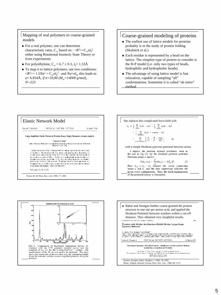
Mapping of real polymers to coarse-grained modelsn For a real polymer, one can determine

characteristic ratio, C∞ based on : <R2>=C∞nl02

either using Rotational Isomeric State Theory or from experiments

n For polyethylene, C∞ = 6.7 ± 0.3, l0= 1.53Ån To map it to lattice polymers, use two conditions:

<R2>= 1.5Na2 = C∞nl02 , and Na=nl0, this leads to

a= 6.834Å, if n=10,00 (Mw=14000 g/mol), N=223

Coarse-grained modeling of proteinsn The earliest use of lattice models for proteins

probably is in the study of protein folding (Skolnick et al.)

n Each residue is represented by a bead on the lattice. The simplest type of protein to consider is the H-P model (i.e. only two types of beads, hydrophilic and hydrophobic beads).

n The advantage of using lattice model is fast relaxation, capable of sampling “all” conformations. Sometime it is called “ab initio” method

Elastic Network Model

Tirion, M. M. Phys. Rev. Lett. 1996, 77, 1905

She replaces this complicated force-field with

with a simple Hookean pairwise potential between atoms

n Bahar and Jernigan further coarse grained the protein structure to one site per amino acid, and applied the Hookean Potential between residues within a cut-off distance. They obtained very insightful results.

Keskin, Jernigan, Bahar, Biophys. J. 2000, 78, 2093Bahar, Atilgan, Demirel, Erman, Phys. Rev. Lett., 1998, 80, 2733

6

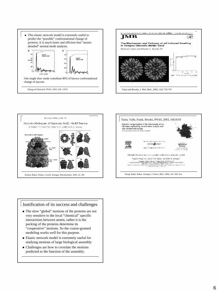
One single slow mode contribute 80% of known conformational change of myosin

n This elastic network model is extremely useful to predict the “possible” conformational change of proteins. It is much faster and efficient that “atomic detailed” normal mode analysis.

Zhang and Doniatch, PNAS, 2003, 100, 13253 Tama and Brooks, J. Mol. Biol., 2002, 318, 733-747

Keskin, Bahar, Flatow, Covell, Jernigan, Biochemistry, 2002, 41, 491

Tama, Valle, Frank, Brooks, PNAS, 2003, 100,9319

Wang, Rader, Bahar, Jernigan, J. Struct. Biol., 2004, 147, 302-314

Justification of its success and challengesn The slow “global” motions of the proteins are not

very sensitive to the local “chemical” specific interactions between atoms, rather it is the packing of the proteins determine its “cooperative” motions. So the coarse-grained modeling works well for this purpose.

n Elastic network model is extremely useful for studying motions of large biological assembly

n Challenges are how to correlate the motions predicted to the function of the assembly.