Classical Mechanics I (Spring 2019): Homework #2 Solution

Due Apr. 18, 2019

[0.5 pt each, total 6 pts]

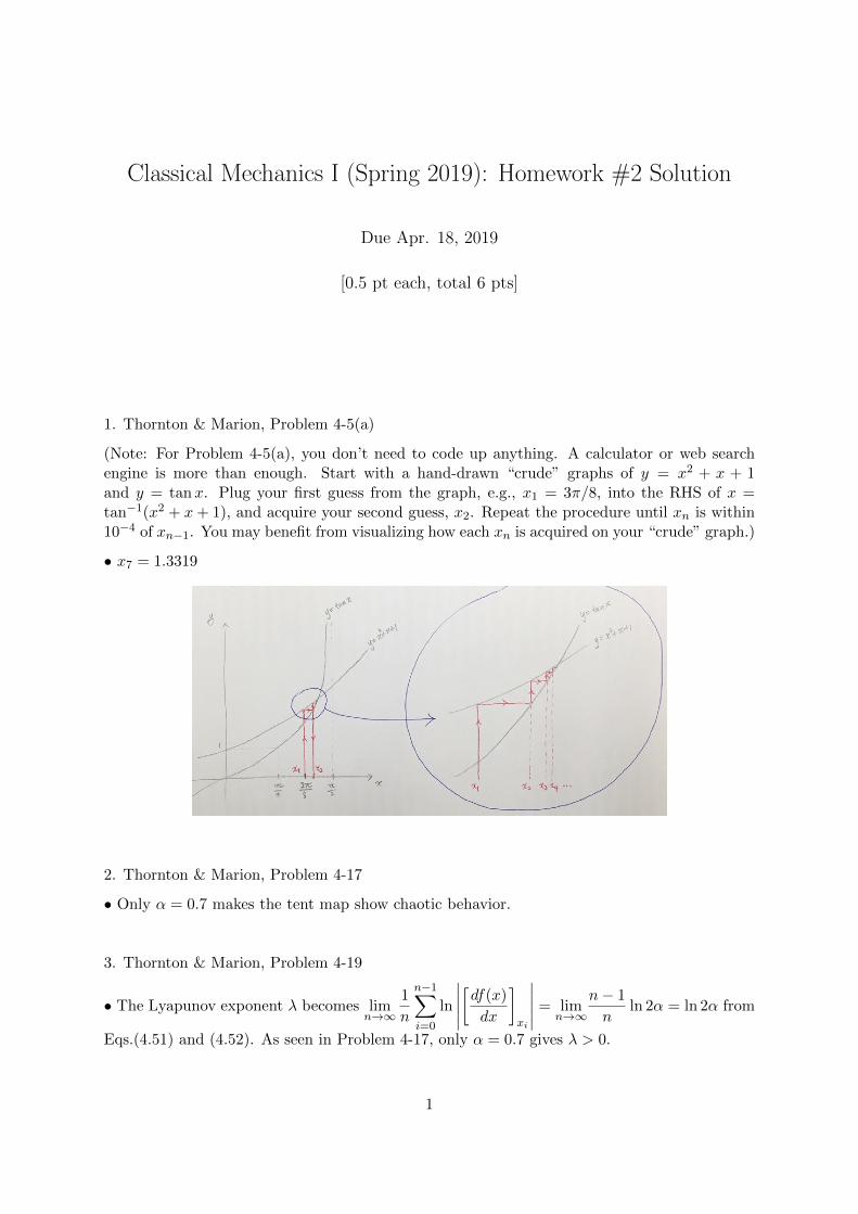
1. Thornton & Marion, Problem 4-5(a)

(Note: For Problem 4-5(a), you don’t need to code up anything. A calculator or web searchengine is more than enough. Start with a hand-drawn “crude” graphs of y = x2 + x + 1and y = tanx. Plug your first guess from the graph, e.g., x1 = 3π/8, into the RHS of x =tan−1(x2 + x+ 1), and acquire your second guess, x2. Repeat the procedure until xn is within10−4 of xn−1. You may benefit from visualizing how each xn is acquired on your “crude” graph.)

• x7 = 1.3319

2. Thornton & Marion, Problem 4-17

• Only α = 0.7 makes the tent map show chaotic behavior.

3. Thornton & Marion, Problem 4-19

• The Lyapunov exponent λ becomes limn→∞

1

n

n−1∑i=0

ln

∣∣∣∣∣[df(x)

dx

]xi

∣∣∣∣∣ = limn→∞

n− 1

nln 2α = ln 2α from

Eqs.(4.51) and (4.52). As seen in Problem 4-17, only α = 0.7 gives λ > 0.

1

4. Thornton & Marion, Problem 4-20

• See e.g., mathworld.wolfram.com/HenonMap.html, or en.wikipedia.org/wiki/Henon map.

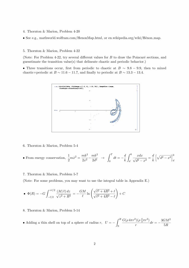
5. Thornton & Marion, Problem 4-22

(Note: For Problem 4-22, try several different values for B to draw the Poincare sections, andguesstimate the transition value(s) that delineate chaotic and periodic behavior.)

• Three transitions occur, first from periodic to chaotic at B ∼ 9.8 − 9.9, then to mixedchaotic+periodic at B ∼ 11.6− 11.7, and finally to periodic at B ∼ 13.3− 13.4.

6. Thornton & Marion, Problem 5-4

• From energy conservation,1

2mx2 =

mk2

2x2−mk

2

2d2→

∫ T

0dt = −d

k

∫ 0

d

xdx√d2 − x2

=d

k

[√d2 − x2

]0d

7. Thornton & Marion, Problem 5-7

(Note: For some problems, you may want to use the integral table in Appendix E.)

• Φ(R) = −G∫ +`/2

−`/2

(M/`) dz√z2 +R2

= −GM`

ln

(√`2 + 4R2 + `√`2 + 4R2 − `

)+ C

8. Thornton & Marion, Problem 5-14

• Adding a thin shell on top of a sphere of radius r, U = −∫ R

0

G(ρ 4πr2)(ρ 43πr

3)

rdr = −3GM2

5R

2

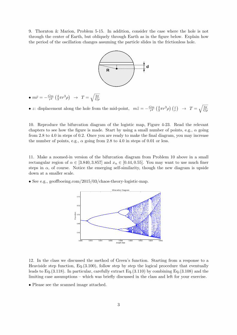
9. Thornton & Marion, Problem 5-15. In addition, consider the case where the hole is notthrough the center of Earth, but obliquely through Earth as in the figure below. Explain howthe period of the oscillation changes assuming the particle slides in the frictionless hole.

• mr = −Gmr2

(43πr

3ρ)→ T =

√3πGρ

• z: displacement along the hole from the mid-point, mz = −Gmr2

(43πr

3ρ) (

zr

)→ T =

√3πGρ

10. Reproduce the bifurcation diagram of the logistic map, Figure 4-23. Read the relevantchapters to see how the figure is made. Start by using a small number of points, e.g., α goingfrom 2.8 to 4.0 in steps of 0.2. Once you are ready to make the final diagram, you may increasethe number of points, e.g., α going from 2.8 to 4.0 in steps of 0.01 or less.

11. Make a zoomed-in version of the bifurcation diagram from Problem 10 above in a smallrectangular region of α ∈ [3.840, 3.857] and xn ∈ [0.44, 0.55]. You may want to use much finersteps in α, of course. Notice the emerging self-similarity, though the new diagram is upsidedown at a smaller scale.

• See e.g., geoffboeing.com/2015/03/chaos-theory-logistic-map.

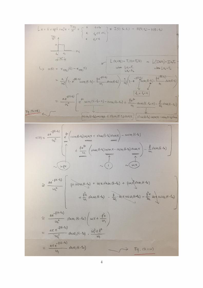
12. In the class we discussed the method of Green’s function. Starting from a response to aHeaviside step function, Eq.(3.100), follow step by step the logical procedure that eventuallyleads to Eq.(3.118). In particular, carefully extract Eq.(3.110) by combining Eq.(3.108) and thelimiting case assumptions – which was briefly discussed in the class and left for your exercise.

• Please see the scanned image attached.

3

4