Classical Hypothesis Testing Theory

Alexander Senf

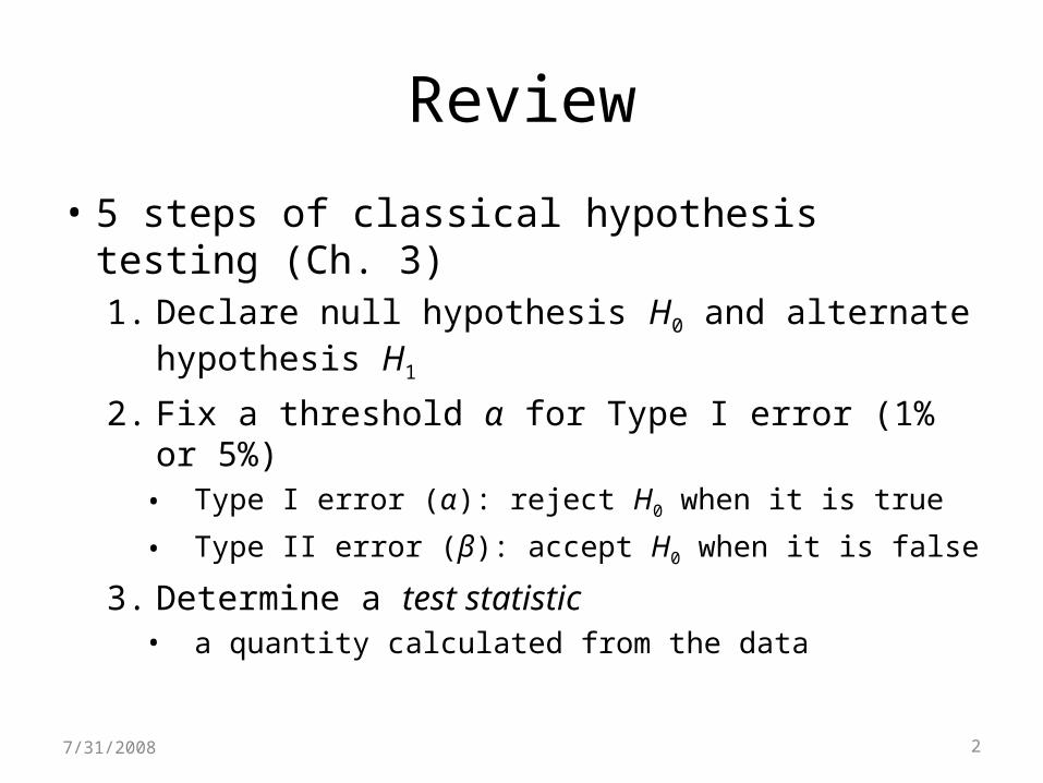
Review

• 5 steps of classical hypothesis testing (Ch. 3)1. Declare null hypothesis H0 and alternate

hypothesis H1

2. Fix a threshold α for Type I error (1% or 5%)• Type I error (α): reject H0 when it is true

• Type II error (β): accept H0 when it is false

3. Determine a test statistic • a quantity calculated from the data

27/31/2008

Review

4. Determine what observed values of the test statistic should lead to rejection of H0

• Significance point K (determined by α)

5. Test to see if observed data is more extreme than significance point K

• If it is, reject H0

• Otherwise, accept H0

37/31/2008

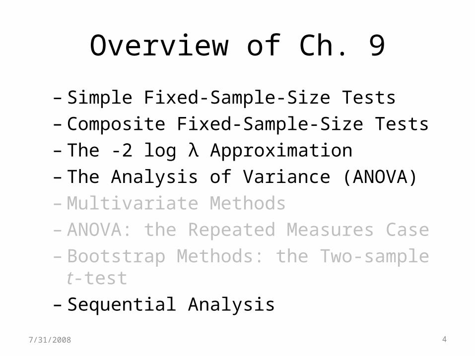
Overview of Ch. 9

– Simple Fixed-Sample-Size Tests– Composite Fixed-Sample-Size Tests– The -2 log λ Approximation– The Analysis of Variance (ANOVA)– Multivariate Methods– ANOVA: the Repeated Measures Case– Bootstrap Methods: the Two-sample t-test– Sequential Analysis

47/31/2008

Simple Fixed-Sample-Size Tests

57/31/2008

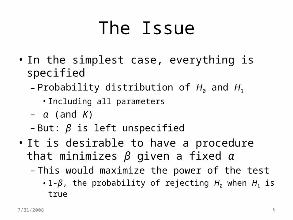
The Issue

• In the simplest case, everything is specified– Probability distribution of H0 and H1

• Including all parameters

– α (and K)– But: β is left unspecified

• It is desirable to have a procedure that minimizes β given a fixed α– This would maximize the power of the test

• 1-β, the probability of rejecting H0 when H1 is true67/31/2008

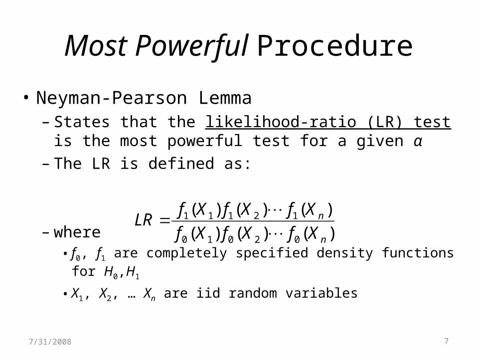
Most Powerful Procedure

• Neyman-Pearson Lemma– States that the likelihood-ratio (LR) test is the most

powerful test for a given α– The LR is defined as:

– where• f0, f1 are completely specified density functions for H0,H1

• X1, X2, … Xn are iid random variables

)()()(

)()()(

02010

12111

n

n

XfXfXf

XfXfXfLR

77/31/2008

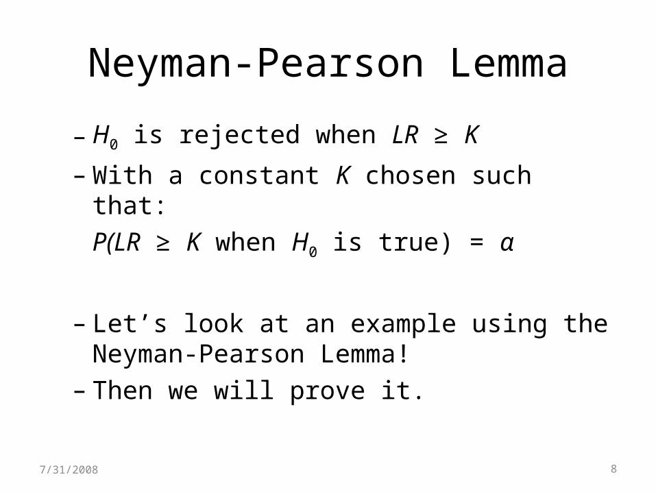
Neyman-Pearson Lemma

– H0 is rejected when LR ≥ K

– With a constant K chosen such that: P(LR ≥ K when H0 is true) = α

– Let’s look at an example using the Neyman-Pearson Lemma!

– Then we will prove it.

87/31/2008

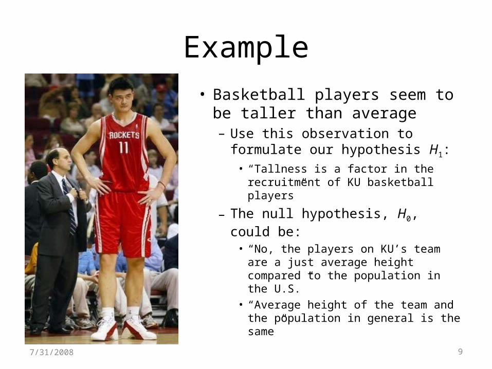
Example• Basketball players seem to be

taller than average– Use this observation to formulate

our hypothesis H1:• “Tallness is a factor in the recruitment

of KU basketball players”

– The null hypothesis, H0, could be:• “No, the players on KU’s team are a

just average height compared to the population in the U.S.”

• “Average height of the team and the population in general is the same”

97/31/2008

Example

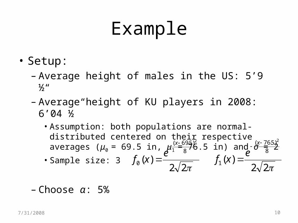
• Setup:– Average height of males in the US: 5’9 ½“– Average height of KU players in 2008: 6’04 ½”

• Assumption: both populations are normal-distributed centered on their respective averages (μ0 = 69.5 in, μ1 = 76.5 in) and σ = 2

• Sample size: 3

– Choose α: 5%22

)(8

)5.76(

1

2

x

exf

22)(

8

)5.69(

0

2

x

exf

107/31/2008

Example

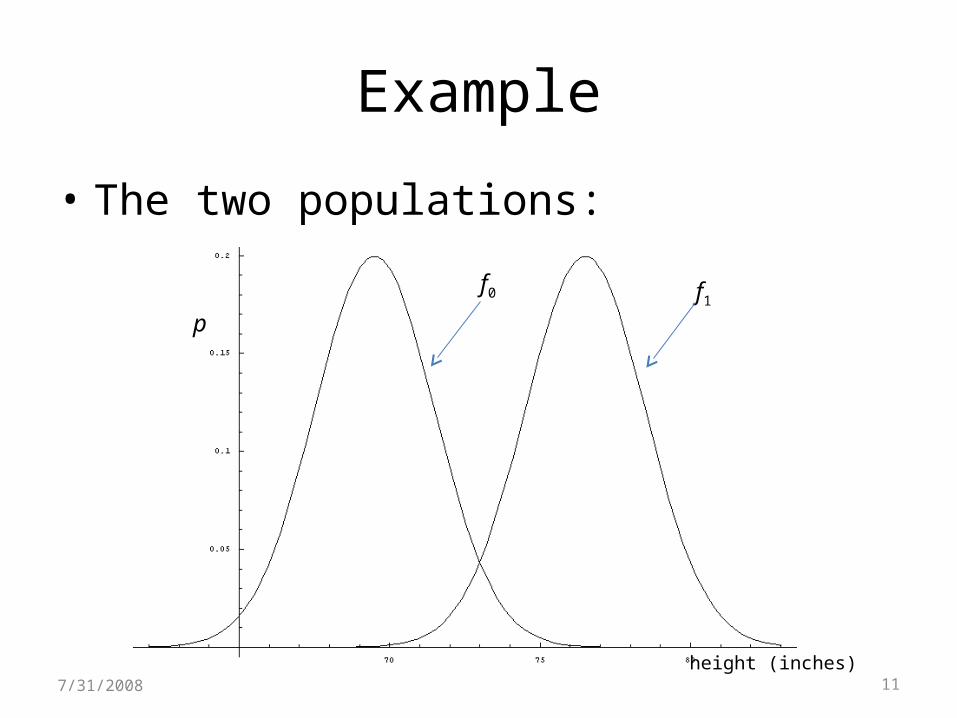
• The two populations:

height (inches)

p

f0 f1

117/31/2008

Example

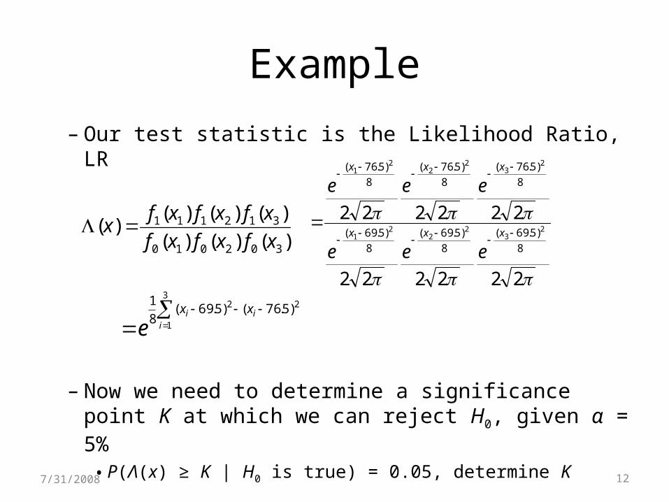
– Our test statistic is the Likelihood Ratio, LR

– Now we need to determine a significance point K at which we can reject H0, given α = 5%

• P(Λ(x) ≥ K | H0 is true) = 0.05, determine K

)()()(

)()()()(

302010

312111

xfxfxf

xfxfxfx

222222

222222

8

)5.69(

8

)5.69(

8

)5.69(

8

)5.76(

8

)5.76(

8

)5.76(

23

22

21

23

22

21

xxx

xxx

eee

eee

3

1

22 )5.76()5.69(8

1

iii xx

e

127/31/2008

Example

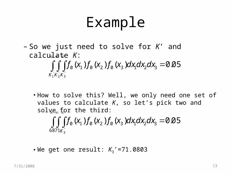
– So we just need to solve for K’ and calculate K:

• How to solve this? Well, we only need one set of values to calculate K, so let’s pick two and solve for the third:

• We get one result: K3’=71.0803

'1

'2

'3

05.0)()()( 321302010

K K K

dxdxdxxfxfxf

6871

321302010'3

05.0)()()(K

dxdxdxxfxfxf

137/31/2008

Example

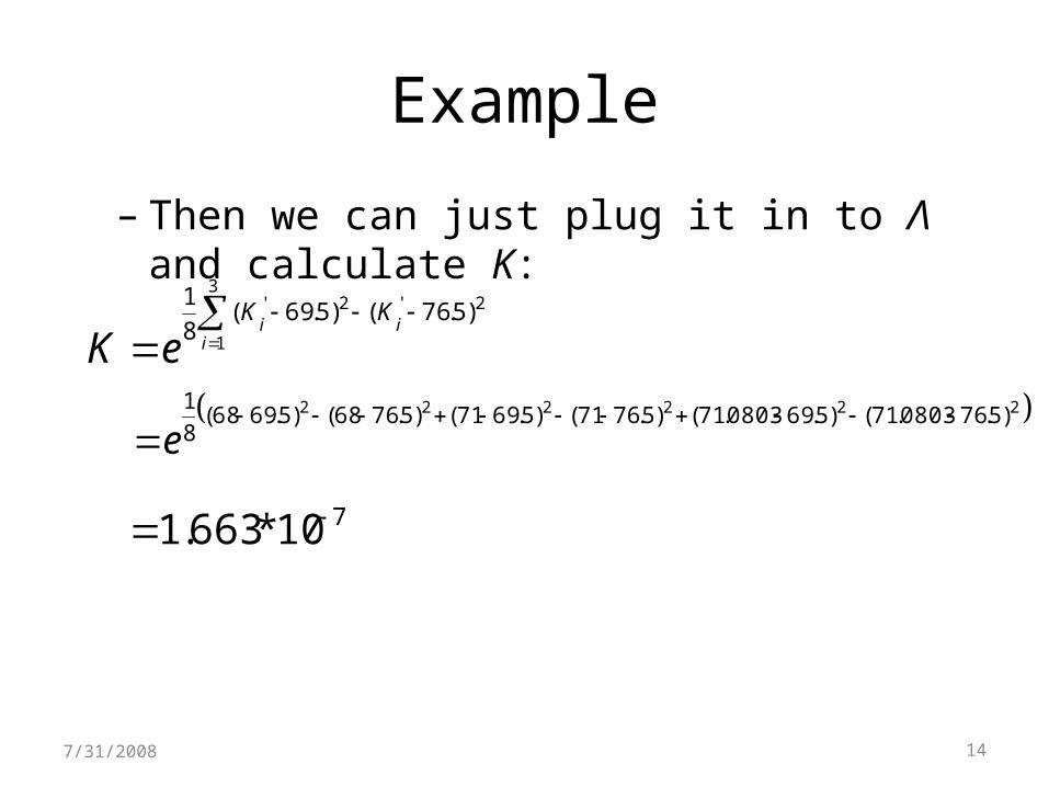
– Then we can just plug it in to Λ and calculate K:

3

1

2'2' )5.76()5.69(8

1

iii

KK

eK

222222 )5.760803.71()5.690803.71()5.7671()5.6971()5.7668()5.6968(8

1

e

710*663.1

147/31/2008

Example

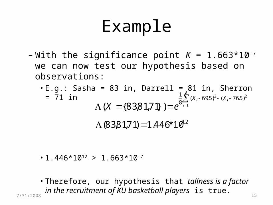
– With the significance point K = 1.663*10-7 we can now test our hypothesis based on observations:

• E.g.: Sasha = 83 in, Darrell = 81 in, Sherron = 71 in

• 1.446*1012 > 1.663*10-7

• Therefore, our hypothesis that tallness is a factor in the recruitment of KU basketball players is true.

1210*446.1)71,81,83(

3

1

22 )5.76()5.69(8

1

})71,81,83{( iii XX

eX

157/31/2008

Neyman-Pearson Proof

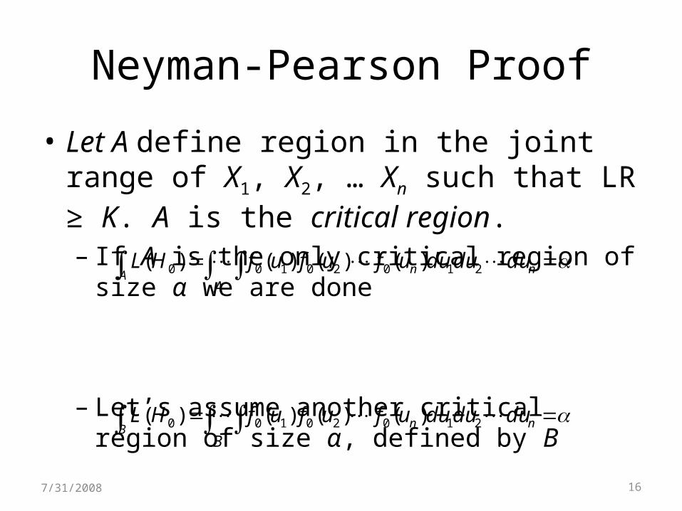
• Let A define region in the joint range of X1, X2, … Xn such that LR ≥ K. A is the critical region.– If A is the only critical region of size α we are done

– Let’s assume another critical region of size α, defined by B

nnAdududuufufufHL 21020100 )()()()(

A

nnBdududuufufufHL 21020100 )()()()(

B

167/31/2008

Proof

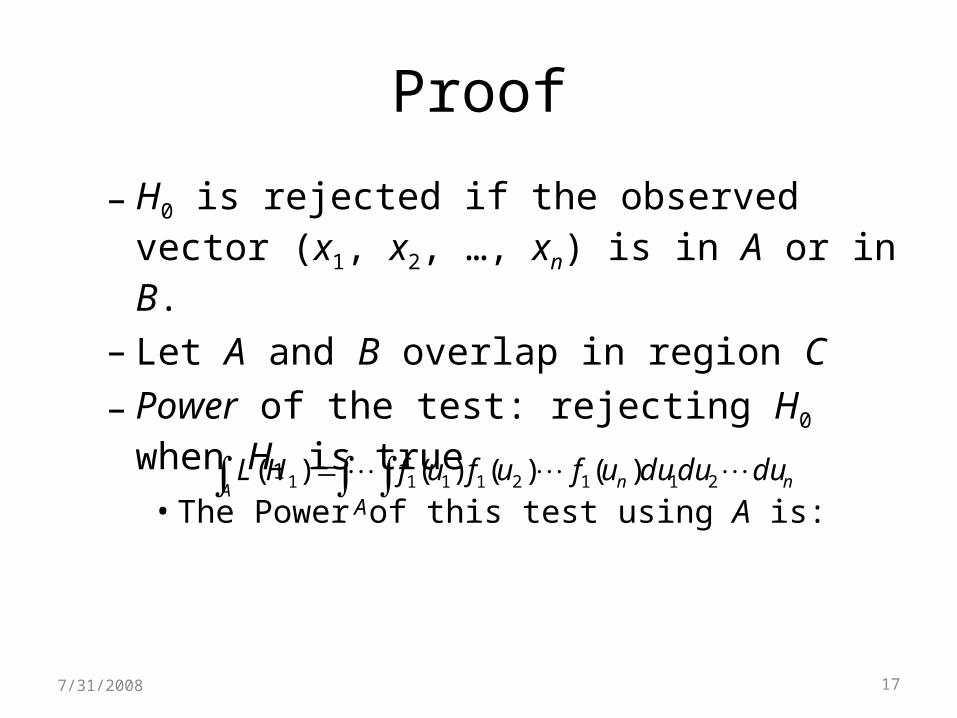
– H0 is rejected if the observed vector (x1, x2, …, xn) is in A or in B.

– Let A and B overlap in region C– Power of the test: rejecting H0 when H1 is true

• The Power of this test using A is:

nnAdududuufufufHL 21121111 )()()()(

A

177/31/2008

Proof

– Define: Δ = ∫AL(H1) - ∫BL(H1) • The power of the test using A minus using B

• Where A\C is the set of points in A but not in C• And B\C contains points in B but not in C

nnnn duduufufduduufuf 11111111 )()()()(A B

nnnn duduufufduduufuf 11111111 )()()()(CA \ CB \

187/31/2008

Proof

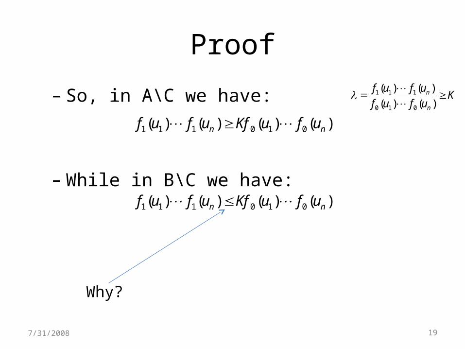
– So, in A\C we have:

– While in B\C we have:

)()()()( 010111 nn ufuKfufuf

)()()()( 010111 nn ufuKfufuf

197/31/2008

Why?

Kufuf

ufuf

n

n )()(

)()(

010

111

Proof

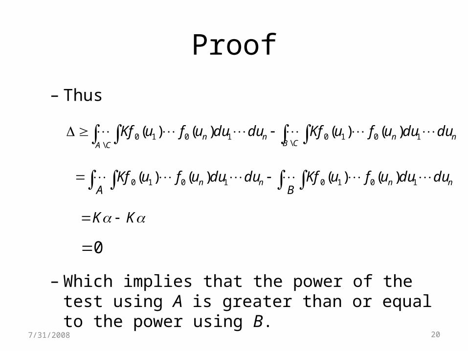
– Thus

– Which implies that the power of the test using A is greater than or equal to the power using B.

nnnn duduufuKfduduufuKf 10101010 )()()()(

nnnn duduufuKfduduufuKf 10101010 )()()()(

CA \ CB \

A B

KK

0

207/31/2008

Composite Fixed-Sample-Size Tests

217/31/2008

Not Identically Distributed

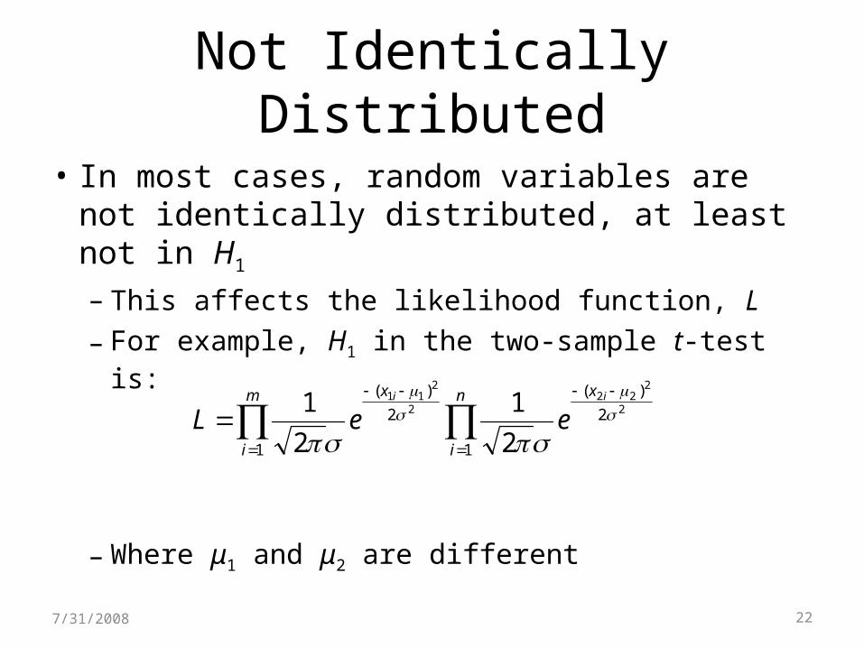
• In most cases, random variables are not identically distributed, at least not in H1

– This affects the likelihood function, L– For example, H1 in the two-sample t-test is:

– Where μ1 and μ2 are different

n

i

xm

i

x ii

eeL1

2

)(

1

2

)(2

222

2

211

2

1

2

1

227/31/2008

Composite

– Further, the hypotheses being tested do not specify all parameters

– They are composite

– This chapter only outlines aspects of composite test theory relevant to the material in this book.

237/31/2008

Parameter Spaces

– The set of values the parameters of interest can take– Null hypothesis: parameters in some region ω– Alternate hypothesis: parameters in Ω– ω is usually a subspace of Ω

• Nested hypothesis case– Null hypothesis nested within alternate hypothesis– This book focuses on this case

• “if the alternate hypothesis can explain the data significantly better we can reject the null hypothesis”

247/31/2008

λ Ratio

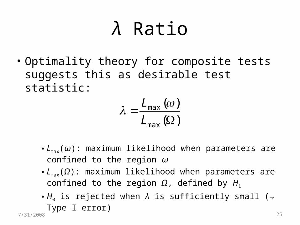
• Optimality theory for composite tests suggests this as desirable test statistic:

• Lmax(ω): maximum likelihood when parameters are confined to the region ω

• Lmax(Ω): maximum likelihood when parameters are confined to the region Ω, defined by H1

• H0 is rejected when λ is sufficiently small (→ Type I error)

)(

)(

max

max

L

L

257/31/2008

Example: t-tests

• The next slides calculate the λ-ratio for the two sample t-test (with the likelihood)

– t-tests later generalize to ANOVA and T2 tests

n

i

xm

i

x ii

eeL1

2

)(

1

2

)(2

222

2

211

2

1

2

1

267/31/2008

Equal Variance Two-Sided t-test

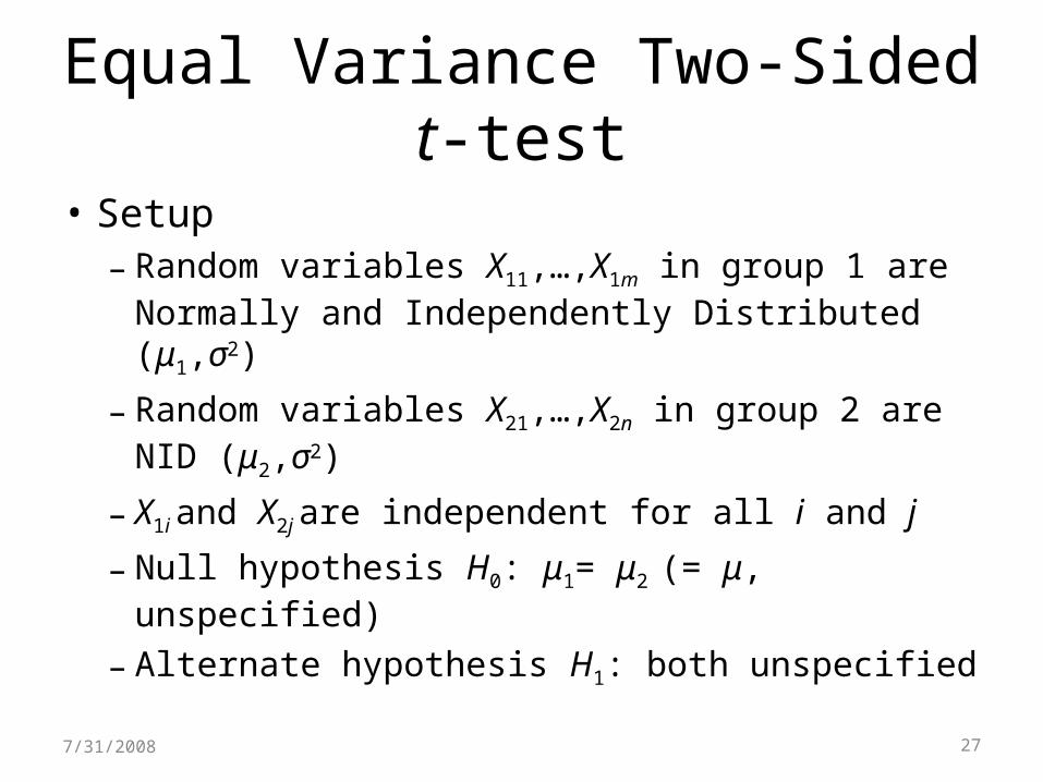
• Setup– Random variables X11,…,X1m in group 1 are

Normally and Independently Distributed (μ1,σ2)

– Random variables X21,…,X2n in group 2 are NID (μ2,σ2)

– X1i and X2j are independent for all i and j

– Null hypothesis H0: μ1= μ2 (= μ, unspecified)

– Alternate hypothesis H1: both unspecified

277/31/2008

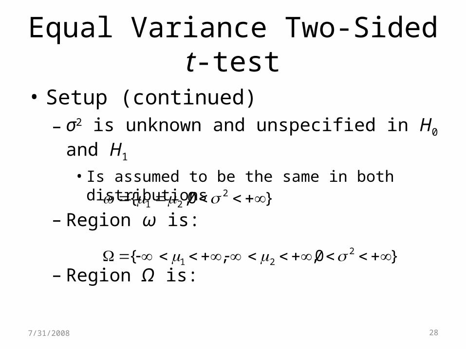
Equal Variance Two-Sided t-test

• Setup (continued)– σ2 is unknown and unspecified in H0 and H1

• Is assumed to be the same in both distributions

– Region ω is:

– Region Ω is: }0,,{ 2

21

}0,{ 221

287/31/2008

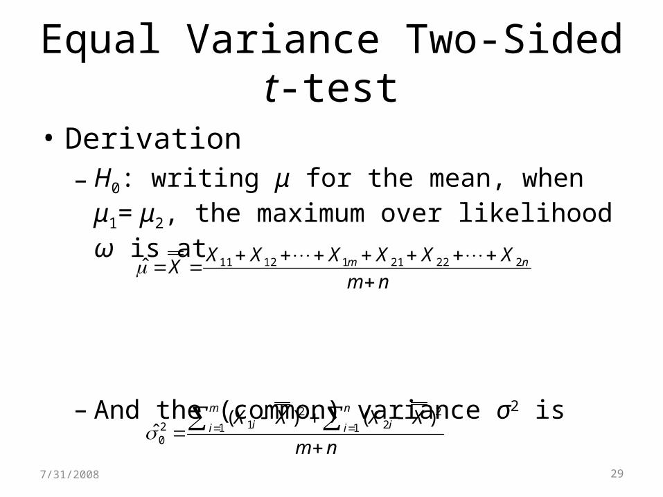
Equal Variance Two-Sided t-test

• Derivation– H0: writing μ for the mean, when μ1= μ2, the

maximum over likelihood ω is at

– And the (common) variance σ2 is

nm

XXXXXXX nm

2222111211ˆ

nm

XXXXn

i i

m

i i

1

221

212

0

)()(

297/31/2008

Equal Variance Two-Sided t-test

– Inserting both into the likelihood function, L

220

max2)ˆ2(

1)(

nm

eL nm

307/31/2008

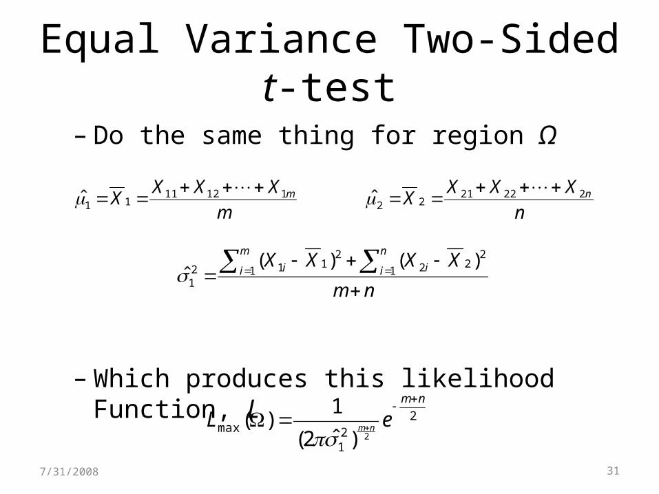
Equal Variance Two-Sided t-test

– Do the same thing for region Ω

– Which produces this likelihood Function, L

m

XXXX m1121111ˆ

n

XXXX n2222122ˆ

nm

XXXXn

i i

m

i i

1

2221

2112

1

)()(

221

max2)ˆ2(

1)(

nm

eL nm

317/31/2008

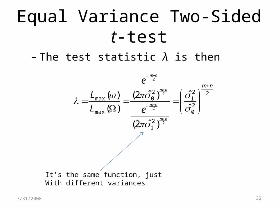
Equal Variance Two-Sided t-test

– The test statistic λ is then

2

20

21

21

20

max

max

ˆ

ˆ

)ˆ2(

)ˆ2(

)(

)(

2

2

2

2

nm

nm

nm

nm

nm

e

e

L

L

It’s the same function, justWith different variances

327/31/2008

Equal Variance Two-Sided t-test

– We can then use the algebraic identity

– To show that

– Where t is (from Ch. 3)

221

2

1

222

1

112

12

2

11 )()()()()( XX

nm

mnXXXXXXXX

n

ii

m

ii

n

ii

m

ii

2

21 2

1nm

nmt

nmS

mnXXT

)( 21

337/31/2008

Equal Variance Two-Sided t-test

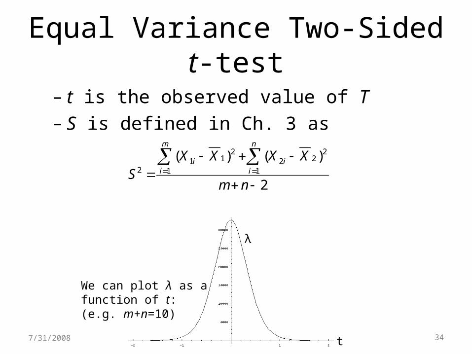
– t is the observed value of T– S is defined in Ch. 3 as

2

)()(1

222

1

211

2

nm

XXXXS

n

ii

m

ii

We can plot λ as afunction of t:(e.g. m+n=10)

t

λ

347/31/2008

Equal Variance Two-Sided t-test

– So, by the monotonicity argument, we can use t2 or |t| instead of λ as test statistic

– Small values of λ correspond to large values of |t|– Sufficiently large |t| lead to rejection of H0

– The H0 distribution of t is known• t-distribution with m+n-2 degrees of freedom

– Significance points are widely available• Once α has been chosen, values of |t| sufficiently large

to reject H0 can be determined

357/31/2008

Equal Variance Two-Sided t-testht

tp:/

/ww

w.s

ocr.

ucla

.edu

/App

lets

.dir/

T-t

able

.htm

l

367/31/2008

Equal Variance One-Sided t-test

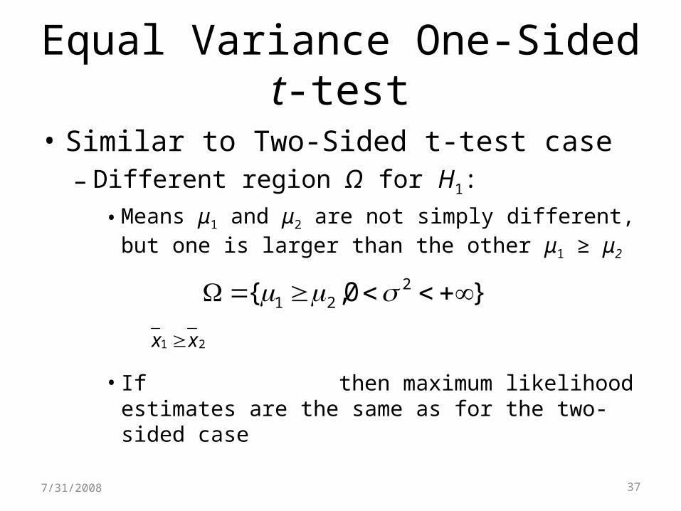
• Similar to Two-Sided t-test case– Different region Ω for H1:

• Means μ1 and μ2 are not simply different, but one is larger than the other μ1 ≥ μ2

• If then maximum likelihood estimates are the same as for the two-sided case

}0,{ 221

21 xx

377/31/2008

Equal Variance One-Sided t-test

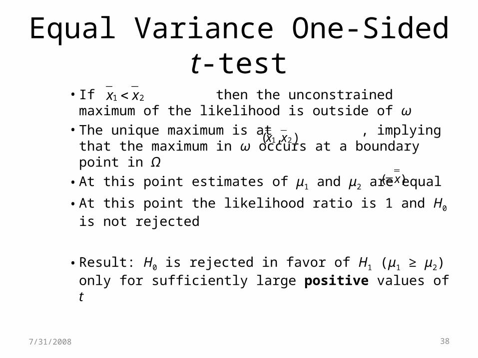
• If then the unconstrained maximum of the likelihood is outside of ω

• The unique maximum is at , implying that the maximum in ω occurs at a boundary point in Ω

• At this point estimates of μ1 and μ2 are equal

• At this point the likelihood ratio is 1 and H0 is not rejected

• Result: H0 is rejected in favor of H1 (μ1 ≥ μ2) only for sufficiently large positive values of t

21 xx

),( 21 xx

)( x

387/31/2008

Example - Revised

• This scenario fits with our original example:– H1 is that the average height of KU basketball

players is bigger than for the general population– One-sided test– We could assume that we don’t know the

averages for H0 and H1

– We actually don’t know σ (I just guessed 2 in the original example)

397/31/2008

Example - Revised

• Updated example:– Observation in group 1 (KU): X1 = {83, 81, 71}

– Observation in group 2: X2 = {65, 72, 70}

– Pick significance point for t from a table: tα = 2.132• t-distribution, m+n-2 = 4 degrees of freedom, α = 0.05

– Calculate t with our observations

– t > tα, so we can reject H0!

185.27673.12

9.27

62122.5

9)693.78(

t

407/31/2008

Comments

• Problems that might arise in other cases– The λ-ratio might not reduce to a function of a

well-known test statistic, such as t– There might not be a unique H0 distribution of λ

– Fortunately, the t statistic is a pivotal quantity• Independent of the parameters not prescribed by H0

– e.g. μ, σ

– For many testing procedures this property does not hold

417/31/2008

Unequal Variance Two-Sided t-test

• Identical to Equal Variance Two-Sided t-test– Except: variances in group 1 and group 2 are no

longer assumed to be identical• Group 1: NID(μ1, σ1

2)

• Group 2: NID(μ2, σ22)

• With σ12 and σ2

2 unknown and not assumed identical

• Region ω = {μ1 = μ2, 0 < σ12, σ2

2 < +∞}

• Ω makes no constraints on values μ1, μ2, σ12, and σ2

2

427/31/2008

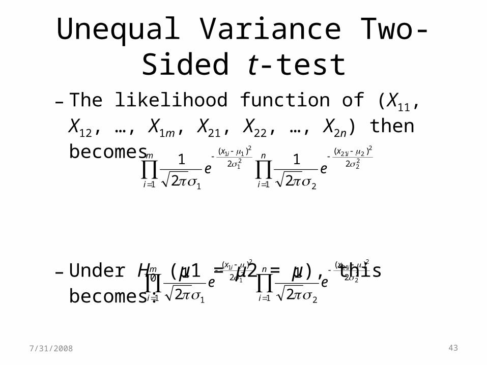
Unequal Variance Two-Sided t-test

– The likelihood function of (X11, X12, …, X1m, X21, X22, …, X2n) then becomes

– Under H0 (μ1 = μ2 = μ), this becomes:

n

i

xm

i

x ii

ee1

2

)(

21

2

)(

1

22

2221

21

211

2

1

2

1

n

i

xm

i

x ii

ee1

2

)(

21

2

)(

1

22

221

21

21

2

1

2

1

437/31/2008

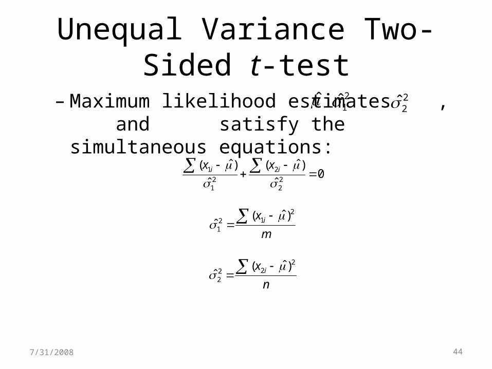
Unequal Variance Two-Sided t-test

– Maximum likelihood estimates , and satisfy the simultaneous equations:

0ˆ

)ˆ(

ˆ

)ˆ(22

2

21

1

ii xx

m

x i

212

1

)ˆ(ˆ

n

x i

222

2

)ˆ(ˆ

21 2

2

447/31/2008

Unequal Variance Two-Sided t-test

– cubic equation in – Neither the λ ratio, nor any monotonic function

has a known probability distribution when H0 is true!

– This does not lead to any useful testing statistic• The t-statistic may be used as reasonably close• However H0 distribution is still unknown, as it depends

on the unknown ratio σ12/σ2

2

• In practice, a heuristic is often used (see Ch. 3.5)

457/31/2008

The -2 log λ Approximation

467/31/2008

The -2 log λ Approximation

• Used when the λ-ratio procedure does not lead to a test statistic whose H0 distribution is known– Example: Unequal Variance Two-Sided t-test

• Various approximations can be used– But only if certain regularity assumptions and

restrictions hold true

477/31/2008

The -2 log λ Approximation

• Best known approximation:– If H0 is true, -2 log λ has an asymptotic chi-square

distribution, • with degrees of freedom equal to the difference in

parameters unspecified by H0 and H1, respectively.

• λ is the likelihood ratio• “asymptotic” = “as the sample size → ∞”

– Provides an asymptotically valid testing procedure

487/31/2008

The -2 log λ Approximation

– Restrictions:• Parameters must be real numbers that can take on

values in some interval• The maximum likelihood estimator is found at a turning

point of the function– i.e. a “real” maximum, not at a boundary point

• H0 is nested in H1 (as in all previous slides)

– These restrictions are important in the proof• I skip the proof…

497/31/2008

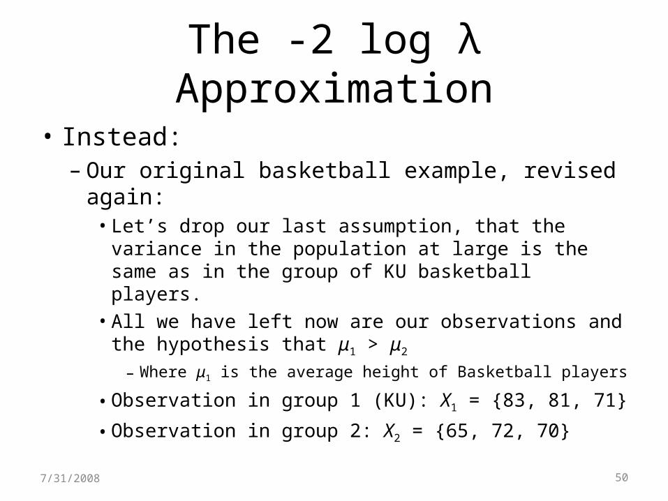
The -2 log λ Approximation

• Instead:– Our original basketball example, revised again:

• Let’s drop our last assumption, that the variance in the population at large is the same as in the group of KU basketball players.

• All we have left now are our observations and the hypothesis that μ1 > μ2

– Where μ1 is the average height of Basketball players

• Observation in group 1 (KU): X1 = {83, 81, 71}

• Observation in group 2: X2 = {65, 72, 70}

507/31/2008

Example – Revised Again

– Using the Unequal Variance One-Sided t-Test– We get:

517/31/2008

The Analysis of Variance (ANOVA)

527/31/2008

The Analysis of Variance (ANOVA)

• Probably the most frequently used hypothesis testing procedure in statistics

• This section– Derives of the Sum of Squares– Gives an outline of the ANOVA procedure– Introduces one-way ANOVA as a generalization of

the two-sample t-test– Two-way and multi-way ANOVA– Further generalizations of ANOVA

537/31/2008

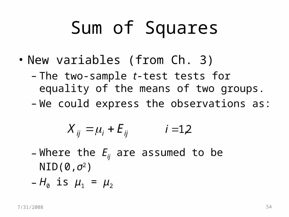
Sum of Squares

• New variables (from Ch. 3)– The two-sample t-test tests for equality of the

means of two groups.– We could express the observations as:

– Where the Eij are assumed to be NID(0,σ2)

– H0 is μ1 = μ2

ijiij EX 2,1i

547/31/2008

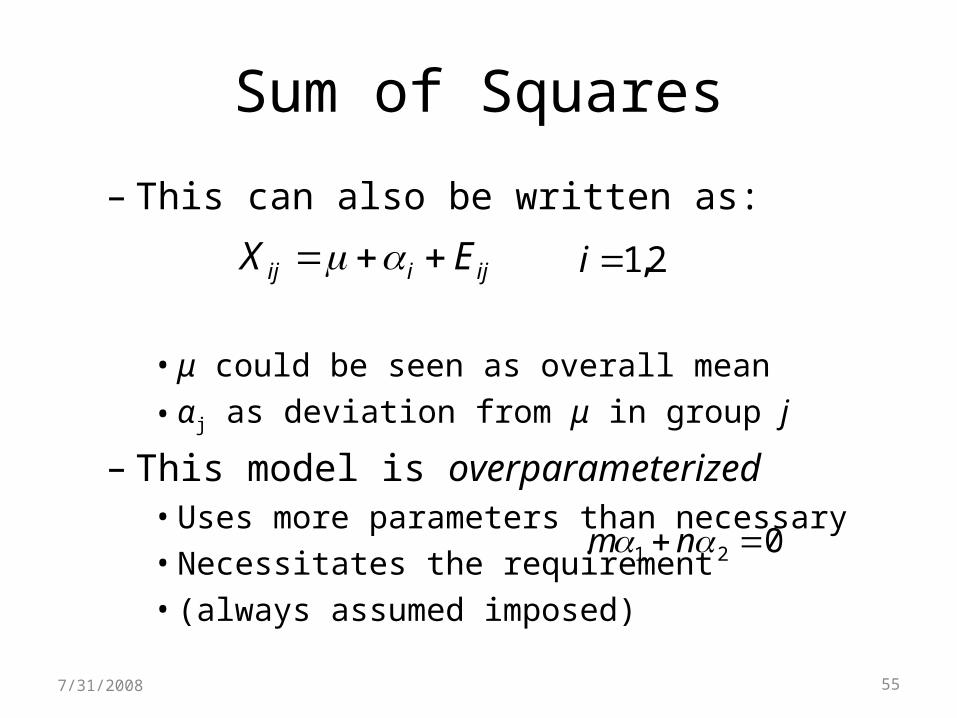
Sum of Squares

– This can also be written as:

• μ could be seen as overall mean• αj as deviation from μ in group j

– This model is overparameterized• Uses more parameters than necessary• Necessitates the requirement• (always assumed imposed)

ijiij EX 2,1i

021 nm

557/31/2008

Sum of Squares

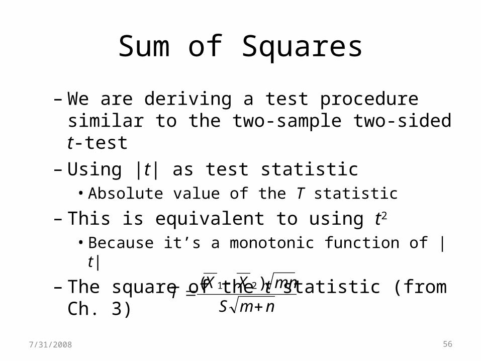
– We are deriving a test procedure similar to the two-sample two-sided t-test

– Using |t| as test statistic• Absolute value of the T statistic

– This is equivalent to using t2

• Because it’s a monotonic function of |t|

– The square of the t statistic (from Ch. 3)

nmS

mnXXT

)( 21

567/31/2008

Sum of Squares

– …can, after algebraic manipulations, be written as F

– where

)2( nmW

BF

m

j

j

m

XX

1

11

n

j

j

n

XX

1

22

nm

XnXmX

21

22

21

221 )()()( XXnXXmXX

nm

mnB

n

jj

m

jj XXXXW

1

222

1

211 )()(

577/31/2008

Sum of Squares

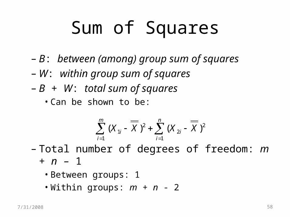
– B: between (among) group sum of squares– W: within group sum of squares– B + W: total sum of squares

• Can be shown to be:

– Total number of degrees of freedom: m + n – 1• Between groups: 1• Within groups: m + n - 2

n

ii

m

ii XXXX

1

22

1

21 )()(

587/31/2008

Sum of Squares

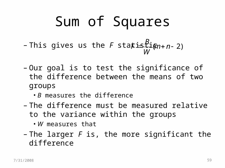
– This gives us the F statistic

– Our goal is to test the significance of the difference between the means of two groups

• B measures the difference

– The difference must be measured relative to the variance within the groups

• W measures that

– The larger F is, the more significant the difference

)2( nmW

BF

597/31/2008

The ANOVA Procedure

• Subdivide observed total sum of squares into several components– In our case, B and W

• Pick appropriate significance point for a chosen Type I error α from an F table

• Compare the observed components to test our hypothesis

607/31/2008

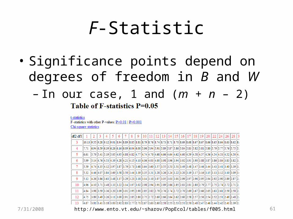
F-Statistic

• Significance points depend on degrees of freedom in B and W– In our case, 1 and (m + n – 2)

http://www.ento.vt.edu/~sharov/PopEcol/tables/f005.html 617/31/2008

Comments

• The two-group case readily generalizes to any number of groups.

• ANOVAs can be classified in various ways, e.g.– fixed effects models– mixed effects models– random effects model– Difference is discussed later– For now we consider fixed effect models

• Parameter αi is fixed, but unknown, in group iijiij EX

627/31/2008

Comments

• Terminology– Although ANOVA contains the word ‘variance’– What we actually test for is a equality in means

between the groups• The different mean assumptions affect the variance,

though

• ANOVAs are special cases of regression models from Ch. 8

637/31/2008

One-Way ANOVA

• One-Way fixed-effect ANOVA• Setup and derivation

– Like two-sample t-test for g number of groups– Observations (ni observations, i=1,2,…,g)

– Using overparameterized model for X

– Eij assumed NID(0,σ2), Σniαi = 0, αi fixed in group i

inii XXX ,,, 21

ijiij EX inj ,,2,1 gi ,,2,1

647/31/2008

One-Way ANOVA

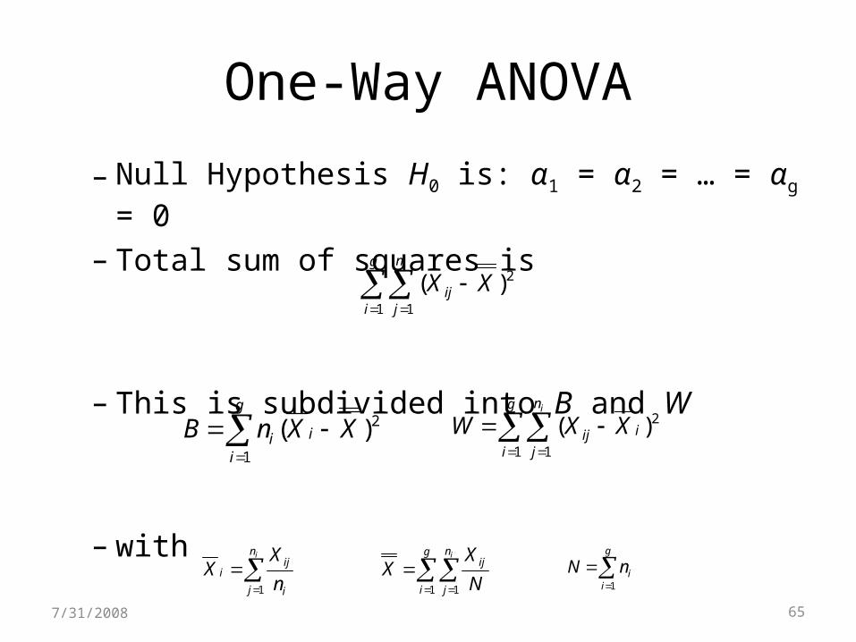
– Null Hypothesis H0 is: α1 = α2 = … = αg = 0

– Total sum of squares is

– This is subdivided into B and W

– with

g

i

n

jij

i

XX1 1

2)(

g

i

ii XXnB1

2)(

g

i

n

j

iij

i

XXW1 1

2)(

in

j i

iji

n

XX

1

g

i

n

j

iji

N

XX

1 1

g

iinN

1

657/31/2008

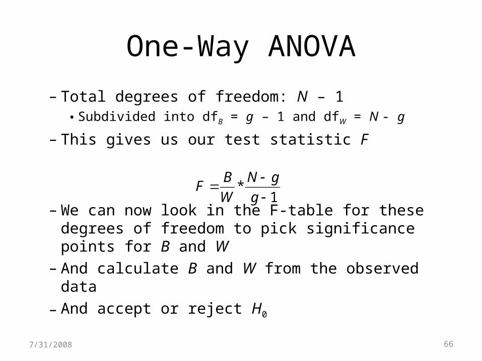
One-Way ANOVA

– Total degrees of freedom: N – 1• Subdivided into dfB = g – 1 and dfW = N - g

– This gives us our test statistic F

– We can now look in the F-table for these degrees of freedom to pick significance points for B and W

– And calculate B and W from the observed data– And accept or reject H0

1*

g

gN

W

BF

667/31/2008

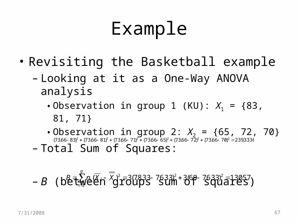
Example

• Revisiting the Basketball example– Looking at it as a One-Way ANOVA analysis

• Observation in group 1 (KU): X1 = {83, 81, 71}

• Observation in group 2: X2 = {65, 72, 70}

– Total Sum of Squares:

– B (between groups sum of squares)

3336.239)7066.73()7266.73()6566.73()7166.73()8166.73()8366.73( 222222

57.130)33.7669(3)33.7633.78(3)( 22

1

2

g

i

ii XXnB

677/31/2008

Example

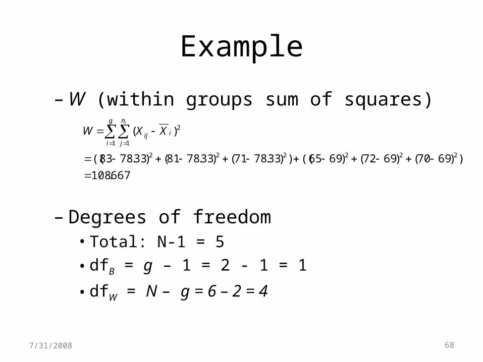
– W (within groups sum of squares)

– Degrees of freedom• Total: N-1 = 5• dfB = g – 1 = 2 - 1 = 1

• dfW = N – g = 6 – 2 = 4

667.108

))6970()6972()6965(())33.7871()33.7881()33.7883((

)(

222222

1 1

2

g

i

n

j

iij

i

XXW

687/31/2008

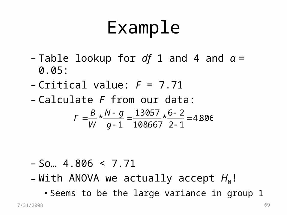
Example

– Table lookup for df 1 and 4 and α = 0.05:– Critical value: F = 7.71– Calculate F from our data:

– So… 4.806 < 7.71– With ANOVA we actually accept H0!

• Seems to be the large variance in group 1

806.412

26*

667.108

57.130

1*

g

gN

W

BF

697/31/2008

Same Example – with Excel

• Screenshots:

707/31/2008

Excel

• Offers most of these tests, built-in

717/31/2008

Two-Way ANOVA

• Two-Way Fixed Effects ANOVA• Overview only (in the scope of this book)• More complicated setup; example:

– Expression levels of one gene in lung cancer patients– a different risk classes

• E.g.: ultrahigh, very high, intermediate, low

– b different age groups– n individuals for each risk/age combination

727/31/2008

Two-Way ANOVA

– Expression levels (our observations): Xijk

• i is the risk class (i = 1, 2, …, a)• j indicates the age group• k corresponds to the individual in each group (k = 1, …, n)

– Each group is a possible risk/age combination

• The number of individuals in each group is the same, n• This is a “balanced” design• Theory for unbalanced designs is more complicated and

not covered in this book

737/31/2008

Two-Way ANOVA

– The Xijk can be arranged in a table:

1 2 3 4

1 n n n n

2 n n n n

3 n n n n

4 n n n n

5 n n n n

ij

Risk category

Age

gro

up

Number of individuals in thisrisk/age group (aka “cell”) This is a two-way table

747/31/2008

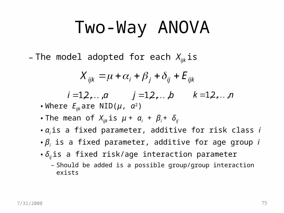
Two-Way ANOVA

– The model adopted for each Xijk is

• Where Eijk are NID(μ, α2)

• The mean of Xijk is μ + αi + βi + δij

• αi is a fixed parameter, additive for risk class i

• βi is a fixed parameter, additive for age group i

• δij is a fixed risk/age interaction parameter– Should be added is a possible group/group interaction exists

ijkijjiijk EX

ai ,,2,1 bj ,,2,1 nk ,,2,1

757/31/2008

Two-Way ANOVA

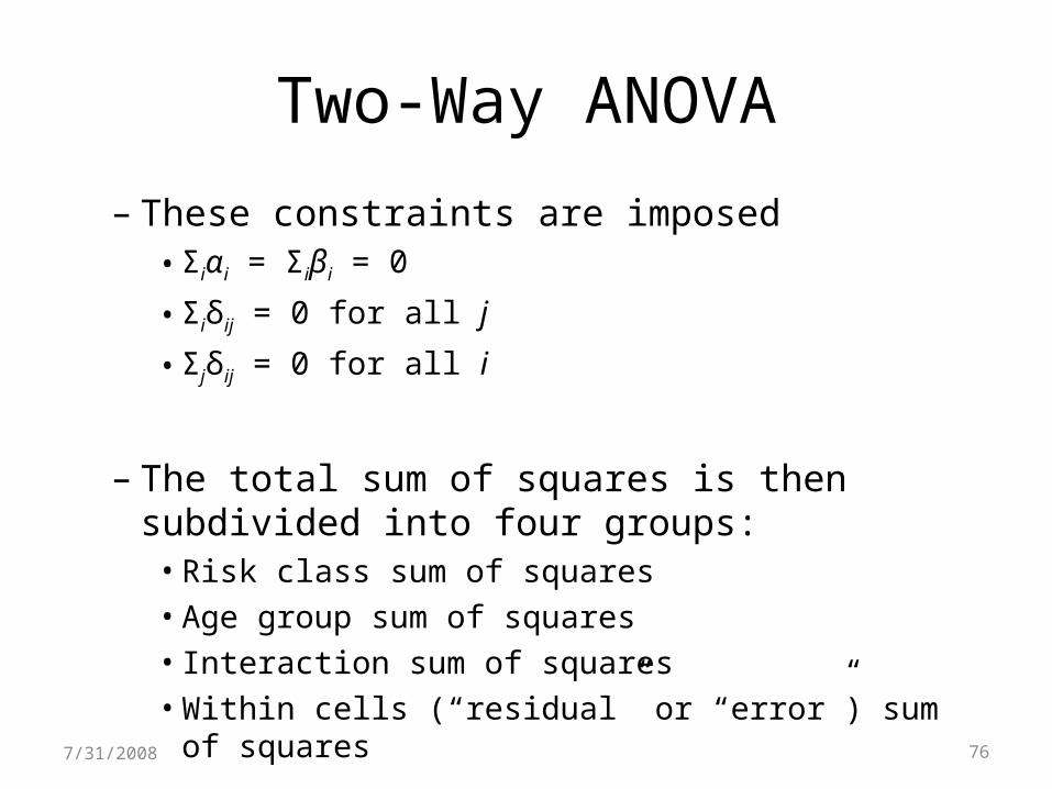
– These constraints are imposed• Σiαi = Σiβi = 0

• Σiδij = 0 for all j

• Σjδij = 0 for all i

– The total sum of squares is then subdivided into four groups:

• Risk class sum of squares• Age group sum of squares• Interaction sum of squares• Within cells (“residual” or “error”) sum of squares 767/31/2008

Two-Way ANOVA

– Associated with each sum of squares• Corresponding degrees of freedom• Hence also a corresponding mean square

– Sum of squares divided by degrees of freedom

– The mean squares are then compared using F ratios to test for significance of various effects

• First – test for a significant risk/age interaction• F-ratio used is ratio of interaction mean square and

within-cells mean square

777/31/2008

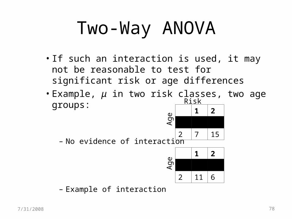
Two-Way ANOVA

• If such an interaction is used, it may not be reasonable to test for significant risk or age differences

• Example, μ in two risk classes, two age groups:

– No evidence of interaction

– Example of interaction

1 2

1 4 12

2 7 15

1 2

1 4 15

2 11 6

Risk

Age

Age

787/31/2008

Multi-Way ANOVA

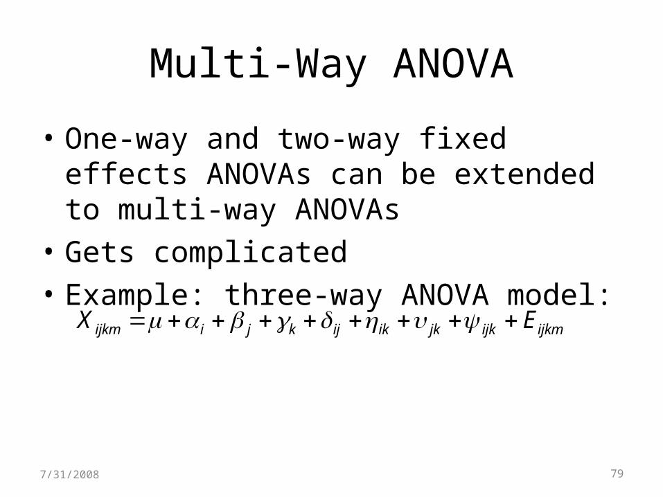
• One-way and two-way fixed effects ANOVAs can be extended to multi-way ANOVAs

• Gets complicated• Example: three-way ANOVA model:

ijkmijkjkikijkjiijkm EX

797/31/2008

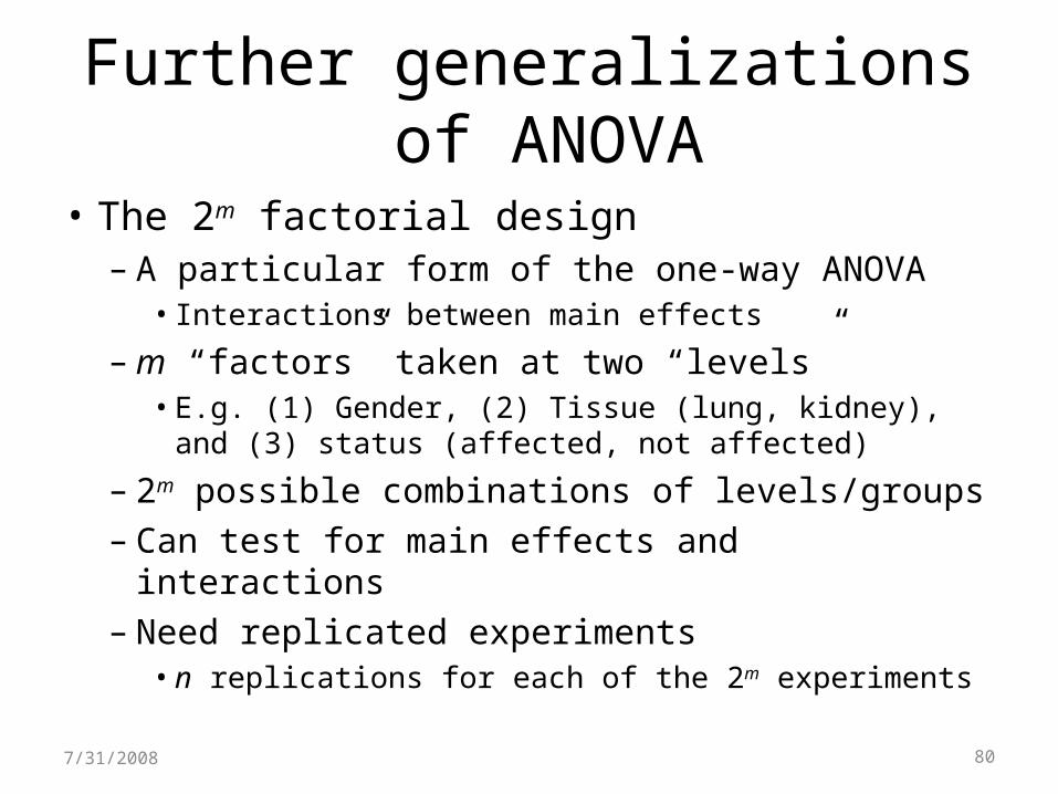
Further generalizations of ANOVA

• The 2m factorial design– A particular form of the one-way ANOVA

• Interactions between main effects

– m “factors” taken at two “levels”• E.g. (1) Gender, (2) Tissue (lung, kidney), and (3) status

(affected, not affected)

– 2m possible combinations of levels/groups– Can test for main effects and interactions– Need replicated experiments

• n replications for each of the 2m experiments807/31/2008

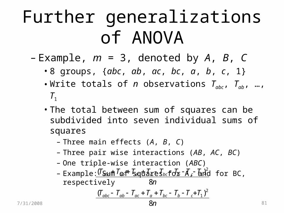
Further generalizations of ANOVA

– Example, m = 3, denoted by A, B, C• 8 groups, {abc, ab, ac, bc, a, b, c, 1}• Write totals of n observations Tabc, Tab, …, T1

• The total between sum of squares can be subdivided into seven individual sums of squares

– Three main effects (A, B, C)– Three pair wise interactions (AB, AC, BC)– One triple-wise interaction (ABC)– Example: Sum of squares for A, and for BC, respectively

n

TTTTTTTT cbbcaacababc

8

)( 21

n

TTTTTTTT cbbcaacababc

8

)( 21

817/31/2008

Further generalizations of ANOVA

– If m ≥ 5 the number of groups becomes large– Then the total number of observations, n2m is large– It is possible to reduce the number of observations

by a process …

• Confounding– Interaction ABC probably very small and not

interesting– So, prefer a model without ABC, reduce data– There are ANOVA designs for that

827/31/2008

Further generalizations of ANOVA

• Fractional Replication– Related to confounding– Sometimes two groups cannot be distinguished

from each other, then they are aliases• E.g. A and BC

– This reduces the need to experiments and data– Ch. 13 talks more about this in the context of

microarrays

837/31/2008

Random/Mixed Effect Models

• So far: fixed effect models– E.g. Risk class, age group fixed in previous example

• Multiple experiments would use same categories• But: what if we took experimental data on several

random days?• The days in itself have no meaning, but a “between

days” sum of squares must be extracted– What if the days turn out to be important?– If we fail to test for it, the significance of our procedure is

diminished.– Days are a random category, unlike risk and age!

847/31/2008

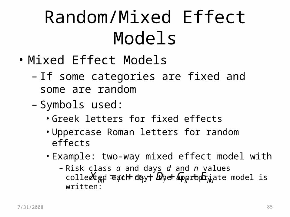
Random/Mixed Effect Models

• Mixed Effect Models– If some categories are fixed and some are random– Symbols used:

• Greek letters for fixed effects• Uppercase Roman letters for random effects• Example: two-way mixed effect model with

– Risk class a and days d and n values collected each day, the appropriate model is written:

iklilliikl EGDX

857/31/2008

Random/Mixed Effect Models

• Random effect model have no fixed categories

• The details on the ANOVA analysis depend on which effects are random and which are fixed

• In a microarray context (more in Ch. 13)– There tend to be several fixed and several random

effects, which complicates the analysis– Many interactions simply assumed zero

867/31/2008

Multivariate Methods

ANOVA: the Repeated Measures Case

Bootstrap Methods: the Two-sample t-test

All skipped …

877/31/2008

Sequential Analysis

887/31/2008

Sequential Analysis

• Sequential Probability Ratio– Sample size not known in advance– Depends on outcomes of successive observations– Some of this theory is in BLAST

• Basic Local Alignment Search Tool

– The book focuses on discreet random variables

897/31/2008

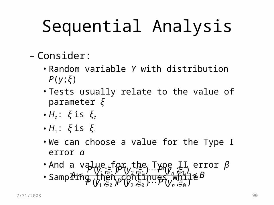
Sequential Analysis

– Consider:• Random variable Y with distribution P(y;ξ)• Tests usually relate to the value of parameter ξ• H0: ξ is ξ0

• H1: ξ is ξ1

• We can choose a value for the Type I error α• And a value for the Type II error β• Sampling then continues while

ByPyPyP

yPyPyPA

n

n );();();(

);();();(

00201

11211

907/31/2008

Sequential Analysis

– A and B are chosen to correspond to an α and β– Sampling continues until the ratio is less than A

(accept H0) or greater than B (reject H0)

– Because these are discreet variables, boundary overshoot usually occurs

• We don’t expect to exactly get values α and β

– Desired values for α and β approximately achieved by using

1

A

1

B

917/31/2008

Sequential Analysis

– It is also convenient to take logarithms, which gives us:

– Using

– We can write

1

log);(

);(log

1log

0

1

i i

i

yP

yP

);(

);(log)(

0

10,1

yP

yPyS

1

log)(1

log 0,1i

iyS

927/31/2008

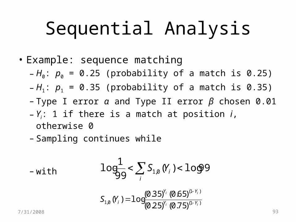
Sequential Analysis

• Example: sequence matching– H0: p0 = 0.25 (probability of a match is 0.25)

– H1: p1 = 0.35 (probability of a match is 0.35)

– Type I error α and Type II error β chosen 0.01– Yi: 1 if there is a match at position i, otherwise 0

– Sampling continues while

– with

i

iYS 99log)(99

1log 0,1

)1(

)1(

0,1 )75.0()25.0(

)65.0()35.0(log)(

ii

ii

YY

YY

iYS

937/31/2008

Sequential Analysis

– S can be seen as the support offered by Yi for H1

– The inequality can be re-written as

– This is actually a random walk with step sizes 0.7016 for a match and -0.2984 for a mismatch

i

iY 581.9)2984.0(581.9

947/31/2008

Sequential Analysis

• Power Function for a Sequential Test– Suppose the true value of the parameter of

interest is ξ– We wish to know the probability that H1 is

accepted, given ξ– This probability is the power Ρ(ξ) of the test

**

*

)()(

)(1)(

11

1

957/31/2008

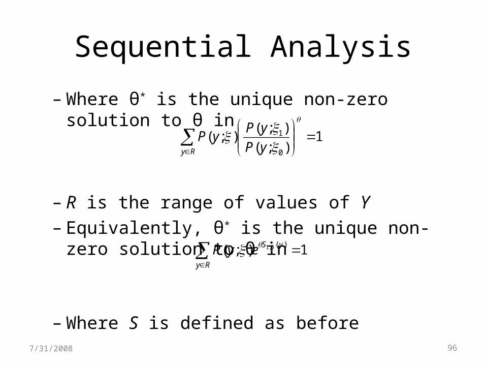
Sequential Analysis

– Where θ* is the unique non-zero solution to θ in

– R is the range of values of Y– Equivalently, θ* is the unique non-zero solution to

θ in

– Where S is defined as before

Ry yP

yPyP 1

);(

);();(

0

1

Ry

ySeyP 1);( )(0,1

967/31/2008

Sequential Analysis

– This is very similar to Ch. 7 – Random Walks– The parameter θ* is the same as in Ch. 7– And it will be the same in Ch 10 – BLAST

– < skipping the random walk part >

977/31/2008

Sequential Analysis

• Mean Sample Size– The (random) number of observations until one or

the other hypothesis is accepted– Find approximation by ignoring boundary

overshoot– Essentially identical method used to find the mean

number of steps until the random walk stops

987/31/2008

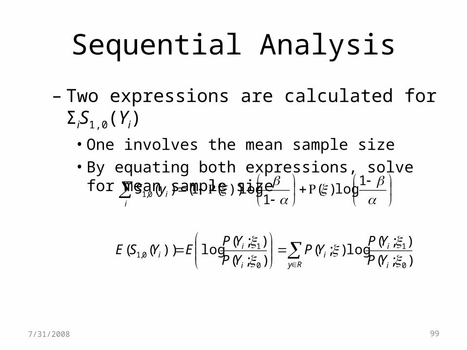
Sequential Analysis

– Two expressions are calculated for ΣiS1,0(Yi)• One involves the mean sample size• By equating both expressions, solve for mean sample

size

1log)(

1log))(1()(0,1

iiyS

Ry i

ii

i

ii YP

YPYP

YP

YPEYSE

);(

);(log);(

);(

);(log))((

0

1

0

10,1

997/31/2008

Sequential Analysis

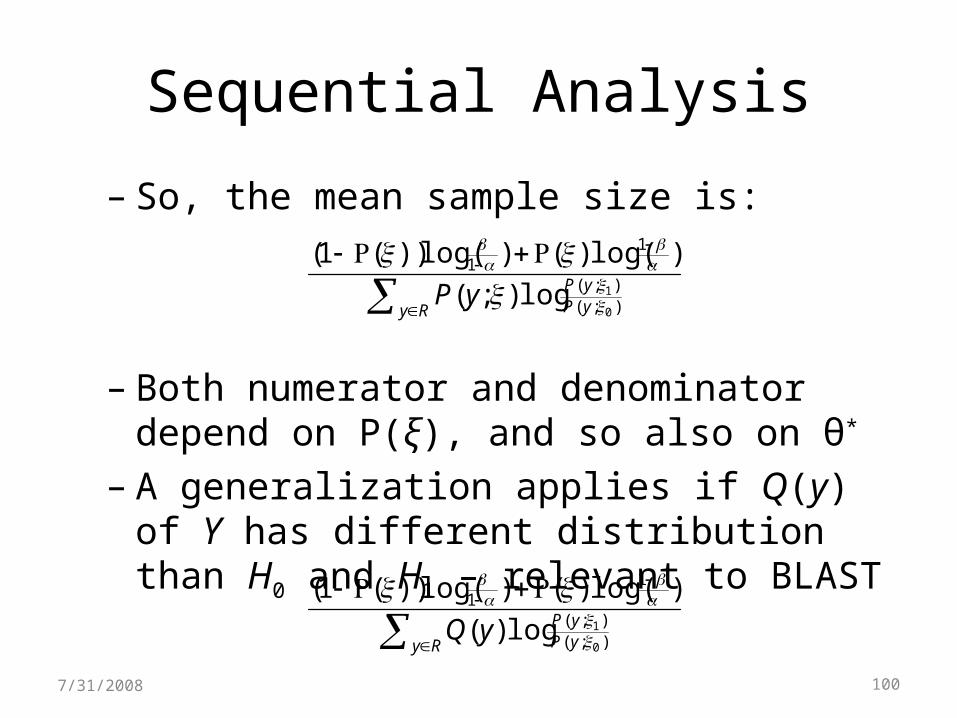
– So, the mean sample size is:

– Both numerator and denominator depend on Ρ(ξ), and so also on θ*

– A generalization applies if Q(y) of Y has different distribution than H0 and H1 – relevant to BLAST

Ry yPyPyP );(

);(

11

0

1log);(

)log()()log())(1(

Ry yPyPyQ );(

);(

11

0

1log)(

)log()()log())(1(

1007/31/2008

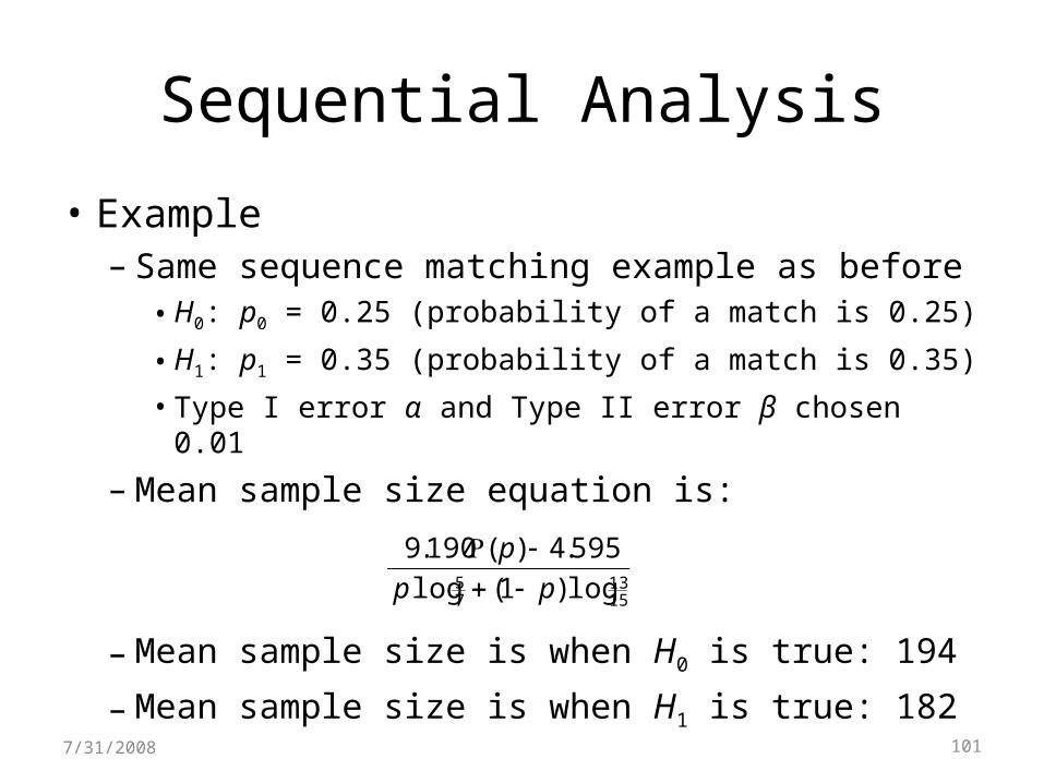
Sequential Analysis

• Example– Same sequence matching example as before

• H0: p0 = 0.25 (probability of a match is 0.25)

• H1: p1 = 0.35 (probability of a match is 0.35)

• Type I error α and Type II error β chosen 0.01

– Mean sample size equation is:

– Mean sample size is when H0 is true: 194

– Mean sample size is when H1 is true: 182

1513

75 log)1(log

595.4)(190.9

pp

p

1017/31/2008

Sequential Analysis

• Boundary Overshoot– So far we assumed no boundary overshoot– In practice, there will almost always be, though

• Exact Type I and Type II errors different from α and β

– Random walk theory can be used to assess how significant the effects of boundary overshoot are

– It can be shown that the sum of Type I and Type II errors is always less than α + β (also individually)

– BLAST deals with this in a novel way -> see Ch. 10

1027/31/2008