Class Handout: Chapter 4 Lyapunov Stability

1

Class Handout: Chapter 4 Lyapunov Stability

2006 Fall

• Lyapunov stability (stability in the sense of Lyapunov): Stability of an equilibrium, Sta-

bility of a trajectory (limit cycle)

• Input-output stability

I. Autonomous Systems

x = f(x)

where f : D ⊂ Rn → Rn is locally Lipschitz, and f(0) = 0.

In most cases, we consider an equilibrium as the origin. (Why?)

Definition 4.1

• We say the origin is stable if, for each ε > 0, there exists δ > 0 such that

‖x(0)‖ ≤ δ ⇒ ‖φ(t, x(0))‖ ≤ ε, t ≥ 0.

(φ(t, x) is the solution starting at x when t = 0.)

• We say the origin is globally attractive if, for each x(0),

‖φ(t, x(0))‖ → 0, t →∞.

• We say the origin is (locally) attractive if there exists δ > 0 such that

‖x(0)‖ < δ ⇒ limt→∞

φ(t, x(0)) = 0.

• We say the origin is globally asymptotically stable (GAS) if it is stable and globally attrac-

tive.

• We say the origin is (locally) asymptotically stable (LAS/AS) if it is stable and (locally)

attractive.

* exponential stability / uniform asymptotic stability

* Issue of global existence of solution in the definition.

* strong / weak stability

Example. Consider a model of pendulum

x1 = x2

x2 = −a sin x1 − bx2, b ≥ 0

CDSL, Seoul Nat’l Univ. September 18, 2006

2

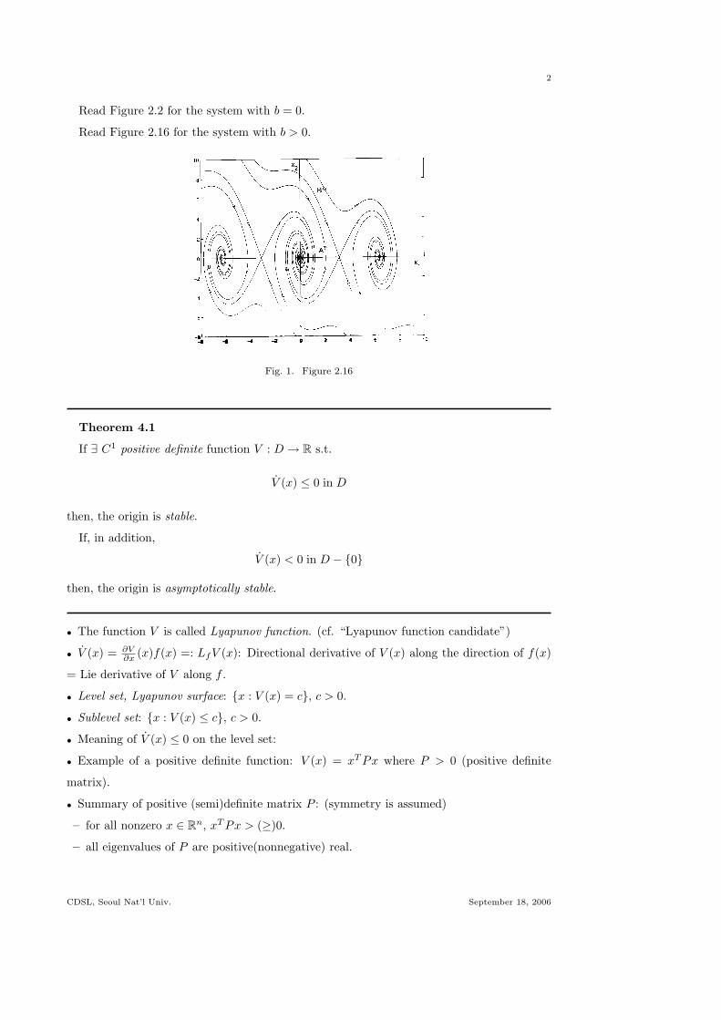
Read Figure 2.2 for the system with b = 0.

Read Figure 2.16 for the system with b > 0.

Fig. 1. Figure 2.16

Theorem 4.1

If ∃ C1 positive definite function V : D → R s.t.

V (x) ≤ 0 in D

then, the origin is stable.

If, in addition,

V (x) < 0 in D − 0

then, the origin is asymptotically stable.

• The function V is called Lyapunov function. (cf. “Lyapunov function candidate”)

• V (x) = ∂V∂x (x)f(x) =: LfV (x): Directional derivative of V (x) along the direction of f(x)

= Lie derivative of V along f .

• Level set, Lyapunov surface: x : V (x) = c, c > 0.

• Sublevel set: x : V (x) ≤ c, c > 0.

• Meaning of V (x) ≤ 0 on the level set:

• Example of a positive definite function: V (x) = xT Px where P > 0 (positive definite

matrix).

• Summary of positive (semi)definite matrix P : (symmetry is assumed)

– for all nonzero x ∈ Rn, xT Px > (≥)0.

– all eigenvalues of P are positive(nonnegative) real.


3

– all the leading principal minors of P are positive (all principal minors of P are nonnega-

tive).

– there is a nonsingular matrix N s.t. P = NT N (there is N ∈ Rm×n s.t. P = NT N).

• Example 4.1:

P =

a 0 1

0 a 2

1 2 a

which is positive definite for a >√

5, and negative definite for a < −√5.

• Lyapunov function approach is a generalization of decreasing energy concept.

• Lyapunov function is not unique.

• Theorem 4.1 is only sufficient. (cf. converse theorem of Section 4.7.)

Example 4.2 For x = −g(x) where g(0) = 0, xg(x) > 0 for x 6= 0. Try with V (x) =∫ x

0g(y)dy. Consider also V (x) = x2 which is simpler. In fact, it is known that, for a scalar

system, V (x) = x2 always becomes a Lyapunov function.

Example 4.3 Consider the pendulum without friction

x1 = x2

x2 = −a sinx1

Try V (x) = a(1 − cos x1) + 12x2

2. Note that, V (0) = 0 and is positive definite only over

−π < x1 < π. What is your conclusion about the stability?

Example 4.4 Consider the pendulum with friction

x1 = x2

x2 = −a sin x1 − bx2, b > 0

Try V (x) = a(1− cos x1) + 12x2

2. What is your conclusion about the stability?

Now try again with

V (x) =12xT Px + a(1− cos x1)

=12

[x1 x2

]p11 p12

p12 p22

x1

x2

+ a(1− cos x1)

For P to be positive definite, we must have

p11 > 0, p11p22 − p212 > 0.


4

Also, Useful facts:

∂

∂xyT x =

∂

∂xxT y = y

∂

∂xyT AT x =

∂

∂xxT Ay = Ay

∂

∂xxT Ax = Ax + AT x

V (x) = (p11x1 + p12x2 + a sin x1)x2 + (p12x1 + p22x2)(−a sin x1 − bx2)

= a(1− p22)x2 sin x1 − ap12x1 sin x1 + (p11 − p12b)x1x2 + (p12 − p22b)x22

To cancel the indefinite terms, we take p22 = 1 and p11 = bp12. Also, let 0 < p12 < b for V (x)

to be positive definite. Let p12 = b/2. Then, V (x) is negative definite on x ∈ R2 : |x1| < π.

Proof. Roughly stated,

V (x(t)) ≤ V (x(0)), ∀t ≥ 0

because V (x(t)) ≤ 0, and this proves the stability. To be precise, the above argument need

to be converted with the norm ‖x‖ to fit in the stability definition.

Given ε > 0, choose r ∈ (0, ε] s.t.

Br = x : ‖x‖ < r ⊂ D.

Let α = min‖x‖=r V (x) > 0. Take β ∈ (0, α) and let

Ωβ = x ∈ Br : V (x) ≤ β ⊂ Br.

Any trajectory started in Ωβ remains in it. (Why?) Thus, the trajectory (solution) exists

for all t ≥ 0. (Why?)

Since V (x) is continuous and V (0) = 0, ∃δ > 0 s.t.

‖x‖ < δ ⇒ V (x) < β.

So, Bδ ⊂ Ωβ ⊂ Br and

‖x(0)‖ < δ ⇒ ‖x(t)‖ < r ≤ ε, ∀t ≥ 0 (Stability).

We now show that x(t) → 0; that is, for each a > 0, ∃T > 0 s.t. ‖x(t)‖ < a for all t > T .

Since for each a > 0, we can choose b s.t. Ωb ⊂ Ba, it is enough to show that V (x(t)) → 0.

(Why?)

Since V (x(t)) is nonincreasing and bounded from below by zero,

V (x(t)) → c ≥ 0 as t →∞.

Suppose c > 0. Let d > 0 s.t. Bd ⊂ Ωc. Let

−γ = maxd≤‖x‖≤r

V (x) < 0.

Then,

V (x(t)) = V (x(0)) +∫ t

0

V (x(s))ds ≤ V (x(0))− γt


5

which implies that V (x(t)) eventually goes below c, which is a contradiction. (Attractivity).

Region of Attraction (Basin of attraction, Domain of attraction)

If the origin is asymptotically stable, we can consider its region of attraction (ROA) =

x : limt→∞ φ(t, x) = 0.Estimating ROA

One (conservative) way to find a subset of ROA is to use the level set of a Lyapunov

function, that is, if Ωc = x : V (x) ≤ c is bounded and contained in D, then every

trajectory starting in Ωc remains in Ωc and approaches the origin as t →∞.

Theorem 4.2 (Barbashin-Krasovskii theorem)

If ∃ C1 positive definite radially unbounded function V : Rn → R s.t.

V (x) < 0 ∀x 6= 0

then, the origin is globally asymptotically stable.

• A positive definite function V : D → R is proper on a set D if, for each c > 0, the sublevel

set Ωc := x : V (x) ≤ c is compact and contained in D. This is equivalent to

V (x) →∞ as x → ∂D.

• radially unbounded = proper on Rn, that is,

V (x) →∞ as ‖x‖ → ∞.

• Radially unboundedness is needed in the theorem. See Exercise 4.8 for a counterexample.

The problem is that for large c, the set Ωc is not necessarily bounded. See Figure 4.4 for

V (x) =x2

1

1 + x21

+ x22.

For small c, Ωc is closed and bounded (because V (x) is continuous and positive definite).

But, for large c, it is unbounded. For Ωc to be in the interior of a ball Br, c must satisfy

c < inf‖x‖≥r V (x). If

l = limr→∞

inf‖x‖≥r

V (x) < ∞

then Ωc will be bounded if c < l.

• If an equilibrium is GAS, it means there is no other equilibrium.

Proof. First, prove that radially unboundedness is equivalent to being proper on Rn; that

is, prove that

V (x) →∞ as ‖x‖ → ∞


6

is equivalent to that, for each c > 0, the set Ωc is compact. (See the textbook.)

Now, for the given initial condition x0, let c = V (x0). Then, Ωc is compact and, since x(t)

remains in Ωc, the previous proof can be employed.

Theorem 4.3 (Chetaev’s Theorem) Instability theorem

If ∃ C1 function V : D → R s.t. V (0) = 0 and V (x) > 0 for some x arbitrarily close to the

origin, and

V (x) > 0 on U := x ∈ Br : V (x) > 0, r > 0,

then, the origin is unstable.

• U is non-empty.

• The boundary of U is the surface V (x) = 0 and ‖x‖ = r. The origin is on the boundary.

(See Figure 4.5).

Proof.

We show that the trajectory x(t), from x(0) = x0 where x0 is in the interior of U , must

leave U .


7

Let a = V (x0) > 0. Then, since V (x) > 0, it follows that V (x(t)) ≥ a for all t ≥ 0. This

means that x(t) cannot cross the boundary (V (x) = 0) of U . We thus show that x(t) will

cross the boundary (‖x‖ = r) of U .

Let γ := minV (x) : x ∈ U and V (x) ≥ a > 0 which exists since it is a minimization of a

continuous function over a compact set. Then,

V (x(t)) = V (x0) +∫ t

0

V (x(s))ds ≥ a +∫ t

0

γds = a + γt.

Hence, x(t) cannot stay in U forever because V (x) is bounded on U , which means x(t) crosses

the curve ‖x‖ = r. Because this happens for any x0 arbitrarily close to the origin, the origin

is unstable.

Example 4.7 Consider

x1 = x1 + g1(x)

x2 = −x2 + g2(x)

where |gi(x)| ≤ k‖x‖22 in the neighborhood of the origin.

Let V (x) = 12 (x2

1 − x22). Then,

V (x) = x21 + x2

2 + x1g1(x)− x2g2(x) ≥ ‖x‖22 − 2k‖x‖32 = ‖x‖22(1− 2k‖x‖2)

So, with Br, r < 1/(2k), we conclude the origin is unstable.

II. The Invariance Principle

Recall Example 4.4 (Pendulum with friction):

x1 = x2

x2 = −a sin x1 − bx2, b > 0

With V (x) = a(1− cosx1) + 12x2

2,

V (x) = −bx22.

For the system to maintain V (x) = 0, the trajectory should be confined to line x2 = 0. But,

this is impossible unless x1 = 0. This makes it possible to claim V (x(t)) → 0 even though

V (x) ≤ 0.


8

• Positive limit point p of the solution x(t): ∃ a seq. tn with tn → ∞ as n → ∞, s.t.,

x(tn) → p as n →∞.

(Ex. AS equilibrium / any point in AS limit cycle)

• Positive limit set of x(t): set of all positive limit points of x(t).

(Ex. AS limit cycle)

• Invariant set M (of the system): a set M s.t.

x(0) ∈ M ⇒ x(t) ∈ M, ∀t ∈ (−∞,∞).

(Ex. limit cycle, equilibrium, ...)

• Positive(negative) invariant set M : in the above, replace t ∈ (−∞,∞) with t ∈ [0,∞)

(t ∈ (−∞, 0]).

(Ex. Ωc with V (x) ≤ 0.)

• Distance of a point x from a set M : dist(x,M) = infy∈M ‖x− y‖ = ‖x‖M

Lemma 4.1

If a sol. x(t) ∈ D is bounded for all t ≥ 0,

then, its positive limit set L+ is nonempty, compact, and invariant.

Moreover, x(t) → L+ as t →∞.

Proof. By Bolzano-Weierstrass theorem, L+ is nonempty because x(t) is bounded.

L+ is bounded because, for any y ∈ L+, there is a seq. ti s.t. x(ti) → y. Since x(t) is

bounded, y is bounded, too.

L+ is closed. Let yi ∈ L+ be a seq. s.t. yi → y. We will prove that y ∈ L+. For each i,

∃ a seq. tij s.t.

tij →∞, x(tij) → yi, as j →∞.

Among the sequence elements tij, we will pick some of them to construct another seq. τias follows: choose τ2 among t2j s.t. τ2 > t12 and ‖x(τ2)−y2‖ < 1/2; choose τ3 among t3js.t. τ3 > t13 and ‖x(τ3)− y3‖ < 1/3; and so on. As a result, τi →∞ and ‖x(τi)− yi‖ < 1/i.

Now, given ε > 0, ∃N1, N2 > 0 s.t.

‖x(τi)− yi‖ <ε

2, ∀i > N1 and ‖yi − y‖ <

ε

2, ∀i > N2.

From the above, we have

‖x(τi)− y‖ < ε, ∀i > N = maxN1, N2,

which implies that y is also a limit point (so, y ∈ L+).


9

L+ is invariant. Let y ∈ L+ and φ(t; y) be the sol. that passes through y at t = 0. We

show that φ(t; y) ∈ L+, ∀t ∈ (−∞,∞). There is a seq. ti s.t. ti →∞ and x(ti) → y. Write

x(ti) = φ(ti;x0) where x0 = x(0). By uniqueness of the sol.,

φ(t + ti;x0) = φ(t; φ(ti;x0)) = φ(t; x(ti)).

Then, for any t ∈ (−∞,∞), (by continuity)

limi→∞

φ(t + ti; x0) = limi→∞

φ(t; x(ti)) = φ(t; y)

which shows φ(t; y) ∈ L+.

We now show that x(t) → L+ as t →∞. Suppose this is not the case. Then, ∃ε > 0 and

ti with ti → ∞ s.t. ‖x(ti)‖L+ > ε. Since x(ti) is bounded, there is a subsequence of it

x(t′i) s.t. x(t′i) → x∗ with some x∗. Then, x∗ must be in L+ because it is a limit point.

This contradicts that ‖x(ti)‖L+ > ε.

Theorem 4.4 (LaSalle’s Invariance Theorem)

Ω ⊂ D: a positively invariant compact set.

V : D → R: C1 function s.t. V (x) ≤ 0 in Ω.

E ⊂ Ω: the set of points s.t. V (x) = 0 in Ω.

M ⊂ E: the largest invariant set in E.

Then, every solution starting in Ω approaches M as t →∞.

Proof. First, since V (x(t)) ≤ 0 and V (x) is bounded below, ∃a s.t. V (x(t)) → a as t →∞.

On the other hand, since Ω is compact and positively invariant, ∃ a positive limit set L+

of x(t) in Ω. We will show that

L+ ⊂ M ⊂ E ⊂ Ω,

which proves the claim since x(t) is bounded, so x(t) → L+.

Pick any p ∈ L+, then there is a seq. tn with tn →∞ and x(tn) → p. Then,

V (p) = limn→∞

V (x(tn)) = a,

which means V (x) = a on L+. Since L+ is invariant, V (x) = 0 on L+, so L+ ⊂ M .

• Only applicable to autonomous (time-invariant) system.

• V (x) need not be positive definite.

• Ω can be found by a sublevel set of V (x), or by other ways.

• If M consists only of the origin, then it is claimed that x(t) → 0. This is done by showing

that no solution can stay identically in E, other than the trivial solution x(t) ≡ 0.


10

Corollary 4.1

V : D → R: C1 positive definite function s.t. V (x) ≤ 0.

S = x ∈ D : V (x) = 0.If no sol. can stay identically in S other than x(t) = 0, then the origin is AS.

Corollary 4.2

In addition, if D = Rn and V (x) is radially unbounded, then the origin is GAS.

Example. Show that the system

x1 = x32

x2 = −x1 − x2

is globally asymptotically stable (using V (x) = 12x2

1 + 14x4

2).

Example 4.10 Consider

y = ay + u

with an adaptive control law

u = −ky, k = γy2, γ > 0.

Taking x1 = y, x2 = k, the closed-loop system becomes

x1 = −(x2 − a)x1

x2 = γx21

The line x1 = 0 is an equilibrium set. (Meaning?)

Consider

V (x) =12x2

1 +12γ

(x2 − b)2, b > a

Then,

V (x) = −x21(x2 − a) + x2

1(x2 − b) = −x21(b− a) ≤ 0.

Then, V (x) is radially unbounded, Ωc is compact for any c > 0. The set E = M = x : x1 =

0. So, we conclude that y(t) → 0.

Since we do not know a, we cannot determine the value b. But, the whole argument still

holds.


11

III. Linear Systems and Linearization

x = Ax, x ∈ Rn

Theorem 4.5 The origin is stable if and only if

• all eigenvalues of A satisfy Re λi ≤ 0

• rank(A − λiI) = n − qi for every eigenvalue with Re λi = 0 and algebraic multiplicity

qi ≥ 2.

The origin is (globally) asymptotically stable if and only if all eigenvalues of A satisfy

Re λi < 0 (Hurwitz or stable matrix).

Proof.

T−1AT = J = blockdiag[J1, J2, · · · , Jr]

where Ji is a Jordan block of order mi corresponding to the eigenvalue λi. Then, E.g., exp(Jt) =

e−λ1t te−λ1t

0 e−λ1t

exp(At) = T exp(Jt)T−1 =

r∑

i=1

mi∑

k=1

tk−1 exp(λit)Rik

where Rik is an appropriate n× n matrix. Note that

x(t) = exp(At)x(0).

With all the above, the claim can be argued.

Example 4.12 Series and parallel connections of the identical model

x =

0 1

−1 0

x +

0

1

u

y =[1 0

]x

The resulting system has the system matrix of

Ap =

0 1 0 0

−1 0 0 0

0 0 0 1

0 0 −1 0

, As =

0 1 0 0

−1 0 0 0

0 0 0 1

1 0 −1 0

.

Both Ap and As has the same e.v. ±j with the algebraic multiplicity qi = 2. Since rank (Ap−jI) = 2, Ap is stable, and since rank (As − jI) = 3, As is unstable.

* “resonance” for the series connection.


12

Consider a quadratic Lyapunov function V (x) = xT Px where P > 0 for the system x = Ax.

Then,

V (x) = xT Px + xT Px = xT (PA + AT P )x = −xT Qx

where Q is symmetric given by

PA + AT P = −Q.

We know that, if Q > 0, then the system is (globally) asymptotically stable. (Why?)

Theorem 4.6 The following are equivalent:

1. A matrix A is Hurwitz.

2. For any Q > 0, ∃ a P > 0 that satisfies

PA + AT P = −Q, (Lyapunov equation).

Moreover, if A is Hurwitz, the P is unique for each Q in the above.

* Q = CT C, where (A,C) is observable, gives the same result. (Exercise 4.22) Home Work!

* Sylvester equation: PA + BP + C = 0.

Proof. (2)→(1): DIY.

(1)→(2): Since A is Hurwitz, define

P :=∫ ∞

0

exp(AT t)Q exp(At) dt,

which is well-defined. (Why?)

From the definition, P is symmetric. In addition, P is positive definite. Indeed, supposing

it is not so, ∃ x 6= 0 s.t. xT Px = 0. Then,∫ ∞

0

xT exp(AT t)Q exp(At)x dt = 0

⇒ exp(At)x ≡ 0 ⇒ x = 0

which is a contradiction.

Therefore,

PA + AT P =∫ ∞

0

exp(AT t)Q exp(At)Adt +∫ ∞

0

AT exp(AT t)Q exp(At)dt

=∫ ∞

0

d

dtexp(AT t)Q exp(At)dt = exp(AT t)Q exp(At)|∞0 = −Q

which means that P is actually a solution of the Lyapunov equation.

Finally, P is unique because, if not, with another solution P 6= P , we have

(P − P )A + AT (P − P ) = 0.


13

Premultiplying by exp(AT t) and postmultiplying by exp(At), we obtain

0 = exp(AT t)[(P − P )A + AT (P − P )] exp(At) =d

dt

exp(AT t)(P − P ) exp(At)

.

Hence,

exp(AT t)(P − P ) exp(At) ≡ a constant, ∀t.

Then,

(P − P ) = exp(AT t)(P − P ) exp(At) → 0 as t →∞,

which proves that P = P .

Pitfall: There’s no mean

value theorem for

multi-variable functions.

That is, for a C1 function

f : Rn → Rn such that

f(0) = 0, it is not true

that there exists q for each

x such that

f(x) = ∂f∂x

(q)x. For

example, try with

f(x1, x2) =

[x21, exp(x1)− 1]T .

x = f(x)

where f is C1 and f(0) = 0.

By the mean value theorem, for each x, ∃zi s.t.

fi(x) = fi(0) +∂fi

∂x(zi)x =

∂fi

∂x(0)x +

[∂fi

∂x(zi)− ∂fi

∂x(0)

]x.

Hence

x = f(x) = Ax + g(x)

where

|gi(x)| ≤∥∥∥∥

∂fi

∂x(zi)− ∂fi

∂x(0)

∥∥∥∥ ‖x‖

which implies that ⇒ Small o notation:

g(x) = o(‖x‖).‖g(x)‖‖x‖ → 0 as ‖x‖ → 0.

Theorem 4.7. (Lyapunov indirect method) Let A = ∂f∂x (0).

1. The origin is locally asymptotically stable if A is Hurwitz.

2. The origin is unstable if Reλi > 0 for one or more of the eigenvalues of A.

• A is called the ‘first order approximation of f(x) at the origin’ or ‘Jacobian of f(x) at the

origin’.

• The theorem does not say anything for the case Reλi ≤ 0 for all i.

Proof. (1) Pick any Q > 0 and solve P s.t. PA + AT P = −Q. Let V (x) = xT Px. Then,

V (x) = xT Pf(x) + fT (x)Px

= xT P [Ax + g(x)] + [xT AT + gT (x)]Px

= xT (PA + AT P )x + 2xT Pg(x)

= −xT Qx + 2xT Pg(x)


14

Since g(x) = o(‖x‖), for any γ > 0, ∃r > 0 s.t.

‖g(x)‖ < γ‖x‖, ∀‖x‖ < r, x 6= 0.

Hence,

V (x) < −xT Qx + 2γ‖P‖‖x‖2, ∀‖x‖ < r, x 6= 0,

≤ −[λmin(Q)− 2γ‖P‖]‖x‖2

which proves (1).

(2) First suppose that A is hyperbolic. Then, ∃ a nonsingular T s.t. ‘Diffeomorphism’ See

Exercise 4.26.

TAT−1 =

−A1 0

0 A2

where Ai’s are Hurwitz. Let z = Tx = [z1; z2]. Then, in z-coordinates, the system becomes

z1 = −A1z1 + g1(z)

z2 = A2z2 + g2(z)

Pick any Q1 > 0 and Q2 > 0, and solve PiAi + ATi Pi = −Qi. Let

V (z) = zT1 P1z1 − zT

2 P2z2.

In the subspace z2 = 0, V (z) > 0 at points arbitrarily close to the origin. Let

U = z ∈ Rn : ‖z‖ ≤ r, V (z) > 0.

In U ,

V (z) = −zT1 (P1A1 + AT

1 P1)z1 + 2zT1 P1g1(z)

− zT2 (P2A2 + AT

2 P2)z2 − 2zT2 P2g2(z)

= zT1 Q1z1 + zT

2 Q2z2 + 2zT [P1g1(z);−P2g2(z)]

≥ λmin(Q1)‖z1‖2 + λmin(Q2)‖z2‖2 − 2‖z‖√‖P1‖2‖g1(z)‖2 + ‖P2‖2‖g2(z)‖2

> (α− 2√

2βγ)‖z‖2 with some α > 0 and β > 0,

which leads to the conclusion. Note that the analysis also can be done in x-coordinates with

P = TT

P1 0

0 −P2

T ; Q = TT

Q1 0

0 Q2

T.

If A has some eigenvalues on the imaginary axis (as well as some eigenvalues in the open The Lyapunov equation

PA + AT P = −Q has, in

fact, a unique solution P if

and only if λi + λj 6= 0 for

all i and j, where λi is an

eigenvalue of A.


15

right-half plane), then consider a matrix [A − (δ/2)I] that is hyperbolic. With it, we find

P = PT and Q > 0 s.t.

P

[A− δ

2I

]+

[A− δ

2I

]T

P = Q.

Again, V (x) = xT Px is positive for points arbitrarily close to the origin. With it, we have

V (x) = xT (PA + AT P )x + 2xT Pg(x)

= xT

[P

(A− δ

2I

)+

(A− δ

2I

)T

P

]x + δxT Px + 2xT Pg(x)

= xT Qx + δV (x) + 2xT Pg(x)

In the set

x ∈ Rn : ‖x‖ ≤ r, V (x) > 0

it follows that

V (x) ≥ λmin(Q)‖x‖2 − 2‖P‖‖x‖‖g(x)‖,

from which the proof is done.

Example 4.14 Consider x = ax3.

Example 4.15 The pendulum system:

x1 = x2

x2 = −a sin x1 − bx2

Inspect stability at (x1, x2) = (0, 0) and (π, 0).

∂f

∂x(x) =

0 1

−a cos x1 −b

Consider two cases: a, b > 0 and a > 0, b = 0 for both equilibria.

IV. Comparison Functions

Definition 4.2

A continuous function α : [0, a) → [0,∞) belongs to class-K if it is strictly increasing and

α(0) = 0.

If a = ∞ and α(r) →∞ as r →∞, then it is called class-K∞.

Definition 4.3


16

A continuous function β : [0, a) × [0,∞) → [0,∞) belongs to class-KL if, for each fixed

s, β(r, s) is of class-K with respect to r, and, for each fixed r, it is decreasing w.r.t. s and

β(r, s) → 0 as s →∞.

Lemma 4.2 Let α1, α2 be class-K functions on [0, a), α3, α4 be class-K∞ functions, β be

a class-KL function.

• α−11 is of class-K on [0, α1(a)).

• α−13 is of class-K∞.

• α1 α2: class-K.

• α3 α4: class-K∞.

• α1(β(α2(r), s)): class-KL.

Lemma 4.3

V : D → R a continuous positive definite function where 0 ∈ D ⊂ Rn.

Br ⊂ D with some r > 0.

Then, ∃ class-K functions α1 and α2 defined on [0, r] s.t.

α1(‖x‖) ≤ V (x) ≤ α2(‖x‖)

for all x ∈ Br.

In addition, if V (x) is radially unbounded, such α1 and α2 can be of class-K∞.

Example. If V (x) = xT Px with P > 0, then α1(s) = λmin(P )s2 and α2(s) = λmax(P )s2.

Proof.

ψ(s) := infs≤‖x‖≤r

V (x) for 0 ≤ s ≤ r

φ(s) := sup‖x‖≤s

V (x) for 0 ≤ s ≤ r

Then, ψ and φ are nondecreasing. So, take class-K α1 and α2 s.t.

α1(s) < ψ(s), φ(s) < α2(s).

Then the claim follows.

The case for V (x) that is radially unbounded is the same with r = ∞.

Lemma 4.4

Scalar system

y = −α(y), y(t0) = y0 ≥ 0


17

where α is locally Lipschitz and of class-K. There exists a unique solution y(t) defined for

all t ≥ t0 s.t.

y(t) = σ(y0, t− t0)

where σ is a class-KL function.

Examples.

• For y = −ky, k > 0, y(t) = y0 exp[−k(t− t0)].

• For y = −ky2, k > 0, y(t) = y0/(ky0(t− t0) + 1).

Proof.

dy

dt= −α(y) ⇒ −

∫ y

y0

dx

α(x)=

∫ t

t0

dt.

Define

η(y) := −∫ y

y0

dx

α(x).

Then, it is strictly decreasing and limy→0 η(y) = ∞ because, from the system equation,

y(t) → 0 as t →∞.

Let c = − limy→∞ η(y) (∈ R ∪ ∞). Then, the range of η(y) is (−c,∞). So, η−1 is

defined on (−c,∞).

Then,

η(y(t))− η(y0) = t− t0

y(t) = η−1(η(y0) + t− t0)

Now, let

σ(r, s) =

η−1(η(r) + s), r > 0

0, r = 0,

which is our class-KL function because Note: Since

η−1(η(x)) = x,

Dxη−1(η(x)) ·Dη(x) = I.

Thus,

∂

∂rσ = Dη−1(η(r) + s)Dη(r)

=α(σ(r, s))

α(r)

∂

∂sσ = Dη−1(η(r) + s)

= −α(σ(r, s))

• it is continuous because limx→∞ η−1(x) = 0,

• it is strictly increasing in r because

∂

∂rσ(r, s) =

α(σ(r, s))α(r)

> 0,

• it is strictly decreasing in s because

∂

∂sσ(r, s) = −α(σ(r, s)) < 0,

• σ(r, s) → 0 as s →∞.


18

An Example: Usefulness in Lyapunov Stability Analysis (Proof of Theorem 4.1)

We have chosen β and δ s.t. Bδ ⊂ Ωβ ⊂ Br. This can also be done as follows: With α1

and α2 s.t.

α1(‖x‖) ≤ V (x) ≤ α2(‖x‖),

choose β ≤ α1(r) and δ ≤ α−12 (β), because

V (x) ≤ β ⇒ α1(‖x‖) ≤ α1(r) ⇔ ‖x‖ ≤ r

‖x‖ ≤ δ ⇒ V (x) ≤ α2(δ) ≤ β.

Now we show (again) that V (x) is negative definite, x(t) tends to zero. There exists a

class-K function α3 s.t. V (x) ≤ −α3(‖x‖). Hence,

V ≤ −α3(α−12 (V )).

Since the differential equation Is the function α3(α−12 (s))

locally Lipschitz? Yes,

without loss of generality

by modifying α2 if

necessary.

y = −α3(α−12 (y)), y(0) = V (x(0))

has a solution y(t) = β(y(0), t) where β is a class-KL function, we know that

V (x(t)) ≤ β(V (x(0)), t).

This is nice because we can go beyond the proof of Theorem 4.1. Now we have

α1(‖x(t)‖) ≤ V (x(t)) ≤ V (x(0)) ≤ α2(‖x(0)‖),

which leads to ‖x(t)‖ ≤ α−11 (α2(‖x(0)‖)). Also,

α1(‖x(t)‖) ≤ V (x(t)) ≤ β(V (x(0)), t) ≤ β(α2(‖x(0)‖), t),

which leads to ‖x(t)‖ ≤ α−11 (β(α2(‖x(0)‖), t)).

V. Nonautonomous Systems

x = f(t, x)

where f : [0,∞)×D → Rn is piecewise continuous in t and locally Lipschitz in x, and

f(t, 0) = 0, ∀t ≥ 0.

An equilibrium at the origin could be a translation of a nonzero equilibrium point or, more

generally, a translation of a nonzero solution of the system. Read p. 147 of the textbook to

see what this means.


19

Example 4.17

x = (6t sin t− 2t)x

x(t) = x(t0) exp[∫ t

t0

(6τ sin τ − 2τ)dτ

]

= x(t0) exp[6 sin t− 6t cos t− t2 − 6 sin t0 + 6t0 cos t0 + t20

]

For any t0, ∃ a constant c(t0) s.t.

|x(t)| < |x(t0)|c(t0), ∀t ≥ t0.

For any ε > 0, take δ = ε/c(t0), which shows that the origin is (not uniformly) stable.

Now consider t0 = 2nπ for n = 0, 1, 2, · · · , and let t = t0 + π. Then,

x(t0 + π) = x(t0) exp[(4n + 1)(6− π)π],

which shows that it is impossible to take δ independently of t0.

Example 4.18

x = − x

1 + t

x(t) = x(t0) exp(∫ t

t0

−11 + τ

dτ

)= x(t0)

1 + t01 + t

In this case, uniformly stable, but not uniformly convergent; that is, given any ε > 0,

∃T = T (ε, t0) > 0 s.t. |x(t)| < ε for t ≥ t0 + T , but T depends on t0.

Definition 4.4 The origin is

• stable if, for each ε > 0, ∃δ(ε, t0) > 0 s.t.

‖x(t0)‖ < δ ⇒ ‖x(t)‖ < ε, ∀t ≥ t0 ≥ 0

• uniformly stable if the origin is stable but the δ is independent of t0

• unstable if it is not stable

• asymptotically stable if the origin is stable and ∃c(t0) > 0 s.t.

x(t) → 0 as t →∞, for all ‖x(t0)‖ < c(t0)

• uniformly asymptotically stable if the origin is uniformly stable, the c above is independent

of t0, and the convergence is uniform, i.e., for each η > 0, ∃T = T (η) > 0 s.t.

‖x(t)‖ < η, ∀t ≥ t0 + T (η), ∀‖x(t0)‖ < c


20

• globally uniformly asymptotically stable (UGAS) if the origin is uniformly stable, δ(ε) can

be chosen to satisfy limε→∞ δ(ε) = ∞, and, for each (η, c), ∃T = T (η, c) > 0 s.t.

‖x(t)‖ < η, ∀t ≥ t0 + T (η, c), ∀‖x(t0)‖ < c

• exponentially stable if ∃ c, k, λ > 0 s.t.

‖x(t)‖ ≤ k‖x(t0)‖e−λ(t−t0), ∀‖x(t0)‖ < c

• globally exponentially stable (GES) if, in addition, c = ∞.

Lemma 4.5 The origin is

• uniformly stable if and only if ∃ a K-function α and c > 0 independent of t0 s.t.

‖x(t)‖ ≤ α(‖x(t0)‖), ∀t ≥ t0 ≥ 0, ∀‖x(t0)‖ < c

• uniformly asymptotically stable if and only if ∃ a KL-function β and c > 0 independent of

t0 s.t.

‖x(t)‖ ≤ β(‖x(t0)‖, t− t0), ∀t ≥ t0 ≥ 0, ∀‖x(t0)‖ < c

• UGAS if and only if ∃ a KL-function β s.t.

‖x(t)‖ ≤ β(‖x(t0)‖, t− t0), ∀t ≥ t0 ≥ 0, ∀x(t0)

Proof. Read Appendix C.6. Homework: Summarize

Appendix C.6.

A function V (t, x) is

• positive definite if V (t, x) ≥ W1(x) where W1 is a positive definite function

• radially unbounded if V (t, x) ≥ W1(x) where W1 is radially unbounded

• decrescent if V (t, x) ≤ W2(x) with a function W2

Theorem 4.8

IF ∃ a C1 V (t, x) s.t.

W1(x) ≤ V (t, x) ≤ W2(x)

∂V

∂t+

∂V

∂xf(t, x) ≤ 0

for all t ≥ 0 and x ∈ D, where W1(x) and W2(x) are continuous positive definite functions, Recall t0 ≥ 0.

THEN x = 0 is uniformly stable.

Proof. Read the book. The key is

x ∈ Br : W2(x) ≤ c ⊂ Ωt,c ⊂ x ∈ Br : W1(x) ≤ c ⊂ Br ⊂ D.


21

Theorem 4.9

• IF, in addition to the assumptions of Theorem 4.8,

∂V

∂t+

∂V

∂xf(t, x) ≤ −W3(x)

for all t ≥ 0 and x ∈ D, where W3(x) is a continuous positive definite function, THEN x = 0

is uniformly asymptotically stable.

In particular, let r and c be s.t. Br ⊂ D and c < min‖x‖=r W1(x). Then,

‖x(t)‖ ≤ β(‖x(t0)‖, t− t0), ∀t ≥ t0 ≥ 0, x(t0) ∈ x ∈ Br : W2(x) ≤ c

where β is a KL-function.

• IF D = Rn and W1(x) is radially unbounded, THEN x = 0 is UGAS.

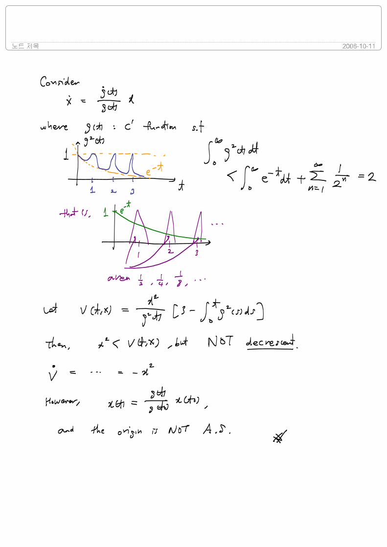
Note. V (t, x) < 0 for x 6= 0 is not enough. W3 is necessary. Consider

x = − 1(1 + t)2

x

Then, with V = x2, V < 0 for x 6= 0, but

x(t) = x(t0)e1/(1+t)−1.

Proof. ∃ a K-function α3 : [0, r] → R s.t.

∂V

∂t+

∂V

∂xf(t, x) ≤ −W3(x) ≤ −α3(‖x‖).

Then,

V ≤ −α3(α−12 (V )) =: −α(V ) ≤ −α(V )

where α is a locally Lipschitz class-K function defined on [0, r].

By the comparison lemma (Lemma 3.4) and Lemma 4.4, ∃ a KL-function σ : [0, r]× [0,∞)

s.t.

V (t, x(t)) ≤ σ(V (t0, x(t0)), t− t0), ∀V (t0, x(t0)) ∈ [0, c].

Thus,

‖x(t)‖ ≤ .... ≤ β(‖x(t0)‖, t− t0)

for x(t0) ∈ x ∈ Br : W2(x) ≤ c, where β is a KL-function. (Fill the blank.)

The rest is omitted. See the book.

Theorem 4.10

IF V is a C1 function s.t.

k1‖x‖a ≤ V (t, x) ≤ k2‖x‖a

∂V

∂t+

∂V

∂xf(t, x) ≤ −k3‖x‖a


22

for all t ≥ 0 and x ∈ D, where ki’s and a are positive constants,

THEN x = 0 is exponentially stable.

If D = Rn, then x = 0 is GES.

Proof.

It can be seen that trajectories starting in k2‖x‖a ≤ c, for sufficiently small c, remain

bounded for all t ≥ t0, and satisfies

V ≤ −k3

k2V.

By the comparison lemma,

V (t, x(t)) ≤ V (t0, x(t0))e−(k3/k2)(t−t0).

Hence,

‖x(t)‖ ≤[V (t, x(t))

k1

]1/a

≤[V (t0, x(t0))e−(k3/k2)(t−t0)

k1

]1/a

≤[k2‖x(t0)‖ae−(k3/k2)(t−t0)

k1

]1/a

=(

k2

k1

)1/a

‖x(t0)‖e−(k3/k2a)(t−t0).

If all the assumptions hold globally, GES follows.

Example 4.19

x = −[1 + g(t)]x3

where continuous g(t) ≥ 0. Take V (x) = 12x2.

Result: UGAS.

Example 4.20

x1 = −x1 − g(t)x2

x2 = x1 − x2

where

0 ≤ g(t) ≤ k, g(t) ≤ g(t).

Take V (t, x) = x21 + [1 + g(t)]x2

2, which satisfies

x21 + x2

2 ≤ V (t, x) ≤ x21 + (1 + k)x2

2.

Then,

V = −2x21 + 2x1x2 − [2 + 2g(t)− g(t)]x2

2 ≤ −2x21 + 2x1x2 − 2x2

2 = −xT Qx


23

where Q > 0.

Result: GES

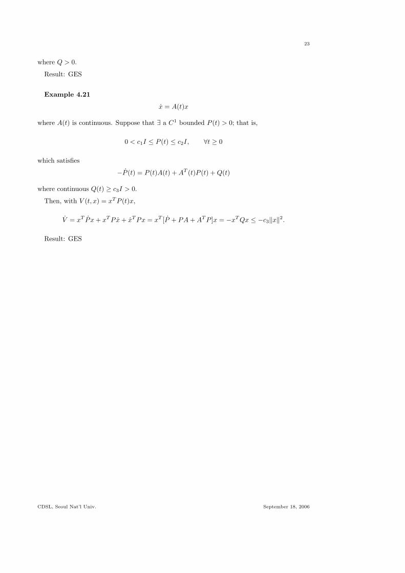
Example 4.21

x = A(t)x

where A(t) is continuous. Suppose that ∃ a C1 bounded P (t) > 0; that is,

0 < c1I ≤ P (t) ≤ c2I, ∀t ≥ 0

which satisfies

−P (t) = P (t)A(t) + AT (t)P (t) + Q(t)

where continuous Q(t) ≥ c3I > 0.

Then, with V (t, x) = xT P (t)x,

V = xT P x + xT Px + xT Px = xT [P + PA + AT P ]x = −xT Qx ≤ −c3‖x‖2.

Result: GES


24

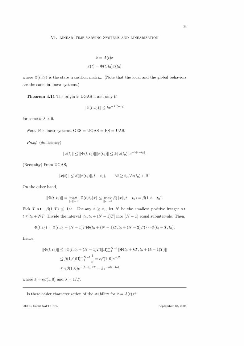
VI. Linear Time-varying Systems and Linearization

x = A(t)x

x(t) = Φ(t, t0)x(t0)

where Φ(t, t0) is the state transition matrix. (Note that the local and the global behaviors

are the same in linear systems.)

Theorem 4.11 The origin is UGAS if and only if

‖Φ(t, t0)‖ ≤ ke−λ(t−t0)

for some k, λ > 0.

Note. For linear systems, GES = UGAS = ES = UAS.

Proof. (Sufficiency)

‖x(t)‖ ≤ ‖Φ(t, t0)‖‖x(t0)‖ ≤ k‖x(t0)‖e−λ(t−t0).

(Necessity) From UGAS,

‖x(t)‖ ≤ β(‖x(t0)‖, t− t0), ∀t ≥ t0, ∀x(t0) ∈ Rn

On the other hand,

‖Φ(t, t0)‖ = max‖x‖=1

‖Φ(t, t0)x‖ ≤ max‖x‖=1

β(‖x‖, t− t0) = β(1, t− t0).

Pick T s.t. β(1, T ) ≤ 1/e. For any t ≥ t0, let N be the smallest positive integer s.t.

t ≤ t0 + NT . Divide the interval [t0, t0 + (N − 1)T ] into (N − 1) equal subintervals. Then,

Φ(t, t0) = Φ(t, t0 + (N − 1)T )Φ(t0 + (N − 1)T, t0 + (N − 2)T ) · · ·Φ(t0 + T, t0).

Hence,

‖Φ(t, t0)‖ ≤ ‖Φ(t, t0 + (N − 1)T )‖Πk=N−1k=1 ‖Φ(t0 + kT, t0 + (k − 1)T )‖

≤ β(1, 0)Πk=N−1k=1

1e

= eβ(1, 0)e−N

≤ eβ(1, 0)e−(t−t0)/T = ke−λ(t−t0)

where k = eβ(1, 0) and λ = 1/T .

Is there easier characterization of the stability for x = A(t)x?


25

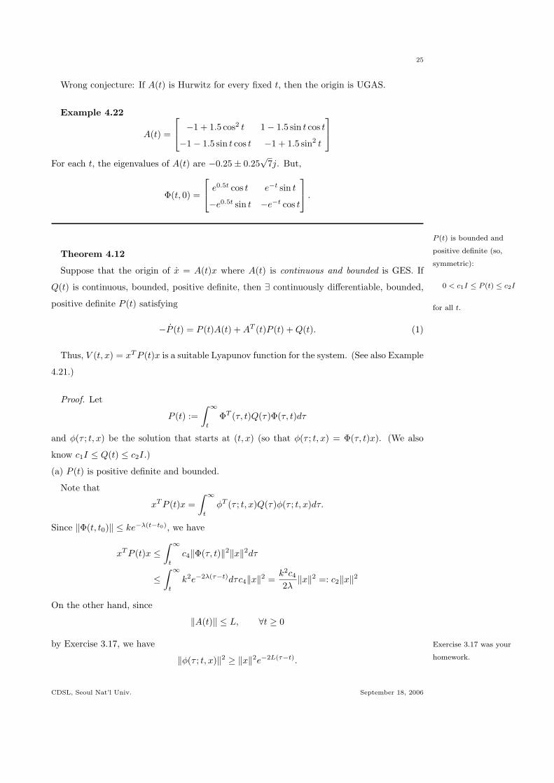
Wrong conjecture: If A(t) is Hurwitz for every fixed t, then the origin is UGAS.

Example 4.22

A(t) =

−1 + 1.5 cos2 t 1− 1.5 sin t cos t

−1− 1.5 sin t cos t −1 + 1.5 sin2 t

For each t, the eigenvalues of A(t) are −0.25± 0.25√

7j. But,

Φ(t, 0) =

e0.5t cos t e−t sin t

−e0.5t sin t −e−t cos t

.

P (t) is bounded and

positive definite (so,

symmetric):

0 < c1I ≤ P (t) ≤ c2I

for all t.

Theorem 4.12

Suppose that the origin of x = A(t)x where A(t) is continuous and bounded is GES. If

Q(t) is continuous, bounded, positive definite, then ∃ continuously differentiable, bounded,

positive definite P (t) satisfying

−P (t) = P (t)A(t) + AT (t)P (t) + Q(t). (1)

Thus, V (t, x) = xT P (t)x is a suitable Lyapunov function for the system. (See also Example

4.21.)

Proof. Let

P (t) :=∫ ∞

t

ΦT (τ, t)Q(τ)Φ(τ, t)dτ

and φ(τ ; t, x) be the solution that starts at (t, x) (so that φ(τ ; t, x) = Φ(τ, t)x). (We also

know c1I ≤ Q(t) ≤ c2I.)

(a) P (t) is positive definite and bounded.

Note that

xT P (t)x =∫ ∞

t

φT (τ ; t, x)Q(τ)φ(τ ; t, x)dτ.

Since ‖Φ(t, t0)‖ ≤ ke−λ(t−t0), we have

xT P (t)x ≤∫ ∞

t

c4‖Φ(τ, t)‖2‖x‖2dτ

≤∫ ∞

t

k2e−2λ(τ−t)dτc4‖x‖2 =k2c4

2λ‖x‖2 =: c2‖x‖2

On the other hand, since

‖A(t)‖ ≤ L, ∀t ≥ 0

by Exercise 3.17, we have Exercise 3.17 was your

homework.‖φ(τ ; t, x)‖2 ≥ ‖x‖2e−2L(τ−t).


26

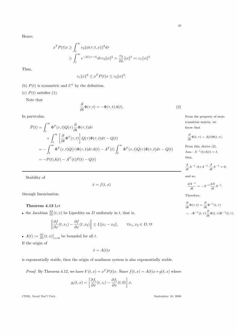
Hence,

xT P (t)x ≥∫ ∞

t

c3‖φ(τ ; t, x)‖2dτ

≥∫ ∞

t

e−2L(τ−t)dτc3‖x‖2 =c3

2L‖x‖2 =: c1‖x‖2

Thus,

c1‖x‖2 ≤ xT P (t)x ≤ c2‖x‖2.

(b) P (t) is symmetric and C1 by the definition.

(c) P (t) satisfies (1).

Note that∂

∂tΦ(τ, t) = −Φ(τ, t)A(t). (2)

In particular, From the property of state

transition matrix, we

know that

∂

∂tΦ(t, τ) = A(t)Φ(t, τ).

From this, derive (2).

Ans.: A−1(t)A(t) = I,

thus,

d

dtA−1·A+A−1· d

dtA−1 = 0,

and so,

dA−1

dt= −A−1 dA

dtA−1.

Therefore,

∂

∂tΦ(τ, t) =

∂

∂tΦ−1(t, τ)

= −Φ−1(t, τ)∂

∂tΦ(t, τ)Φ−1(t, τ).

P (t) =∫ ∞

t

ΦT (τ, t)Q(τ)∂

∂tΦ(τ, t)dτ

+∫ ∞

t

[∂

∂tΦT (τ, t)

]Q(τ)Φ(τ, t)dτ −Q(t)

= −∫ ∞

t

ΦT (τ, t)Q(τ)Φ(τ, t)dτA(t)−AT (t)∫ ∞

t

ΦT (τ, t)Q(τ)Φ(τ, t)dτ −Q(t)

= −P (t)A(t)−AT (t)P (t)−Q(t)

Stability of

x = f(t, x)

through linearization.

Theorem 4.13 Let

• the Jacobian ∂f∂x (t, x) be Lipschitz on D uniformly in t, that is,∥∥∥∥

∂f

∂x(t, x1)− ∂f

∂x(t, x2)

∥∥∥∥ ≤ L‖x1 − x2‖, ∀x1, x2 ∈ D, ∀t

• A(t) := ∂f∂x (t, x)

∣∣x=0

be bounded for all t.

If the origin of

x = A(t)x

is exponentially stable, then the origin of nonlinear system is also exponentially stable.

Proof. By Theorem 4.12, we have V (t, x) = xT P (t)x. Since f(t, x) = A(t)x+g(t, x) where

gi(t, x) =[∂fi

∂x(t, zi)− ∂fi

∂x(t, 0)

]x,


27

with which, we have

‖g(t, x)‖ ≤ L‖x‖2.

So,

V (t, x) = xT (PA + AT P + P )x + 2xT Pg(t, x)

= −xT Q(t)x + 2xT P (t)g(t, x)

≤ −c3‖x‖2 + 2c2L‖x‖3

≤ −(c3 − 2c2Lρ)‖x‖2

for all ‖x‖ < ρ.

VII. Converse Theorems

What is converse theorem?

Theorem 4.14 Consider

x = f(t, x)

where f is C1 on [0,∞)×D, D = Br, and ∂f∂x (t, x) is bounded on D uniformly in t.

IF

‖x(t)‖ ≤ k‖x(t0)‖e−λ(t−t0), ∀x(t0) ∈ D0, ∀t ≥ t0 ≥ 0,

where D0 = Br0 with r0 < r/k,

THEN ∃ a C1 function V : [0,∞)×D0 → R s.t.

c1‖x‖2 ≤ V (t, x) ≤ c2‖x‖2∂V

∂t(t, x) +

∂V

∂xf(t, x) ≤ −c3‖x‖2

∥∥∥∥∂V

∂x

∥∥∥∥ ≤ c4‖x‖

Moreover, if the origin is GES, then global Lyapunov function V (t, x) exists, and if the

system is autonomous, then V can be independent of t.

Proof. DIY while comparing the proof of Theorem 4.12. A Lyapunov function will be

given by

V (t, x) =∫ t+δ

t

φT (τ ; t, x)φ(τ ; t, x)dτ.


x = f(t, x)


28


Suppose also that ∂f∂x (t, x) is Lipschitz on D uniformly in t.

The origin is ES if and only if the origin of

x =∂f

∂x(t, x)

∣∣x=0

x

is ES.

Corollary 4.3 Consider

x = f(x)

where f(x) is C1 and f(0) = 0.

The origin is ES if and only if A = ∂f∂x (0) is Hurwitz.

* Note that AS (rather than ES) has no such simple relation as above.

Proof. DIY.


x = f(t, x)


IF

‖x(t)‖ ≤ β(‖x(t0)‖, t− t0), ∀x(t0) ∈ D0, ∀t ≥ t0 ≥ 0,

where D0 = Br0 with r0 s.t. β(r0, 0) < r,

THEN ∃ a C1 function V : [0,∞)×D0 → R s.t.

α1(‖x‖) ≤ V (t, x) ≤ α2(‖x‖)∂V

∂t(t, x) +

∂V

∂xf(t, x) ≤ −α3(‖x‖)

∥∥∥∥∂V

∂x

∥∥∥∥ ≤ α4(‖x‖)

If the system is autonomous, then V can be independent of t.


x = f(x)

where f is locally Lipschitz.

IF the origin is AS with its region of attraction RA,

THEN ∃ a C∞ positive definite function V (x) (defined on RA) s.t.

V (x) →∞ as x → ∂RA (V (x) is proper on RA)

LfV (x) ≤ −W (x)


29

for all x ∈ RA where W (x) is a continuous positive definite function defined on RA.

When RA = Rn, V (x) is radially unbounded.

Proofs of Theorems 4.16 and 17: Skipped.


30

VIII. Boundedness and Ultimate Boundedness

x = f(t, x)

Case 1: V (x(t)) ≤ 0

Case 2: V (x(t)) ≤ −V (x) + d (e.g., x = −x + δ sin t)

Definition 4.6 The solution x(t) is

• uniformly bounded if ∃c > 0, indep. of t0, and for every a ∈ (0, c), ∃β = β(a) > 0, indep.

of t0, s.t.

‖x(t0)‖ ≤ a ⇒ ‖x(t)‖ ≤ β, ∀t ≥ t0

• globally uniformly bounded if c = ∞ in the above,

• uniformly ultimately bounded with ultimate bound b if ∃b, c > 0, indep. of t0, and for every

a ∈ (0, c), ∃T = T (a, b) ≥ 0, indep. of t0, s.t.

‖x(t0)‖ ≤ a ⇒ ‖x(t)‖ ≤ b, ∀t ≥ t0 + T

• globally uniformly ultimately bounded if c = ∞ in the above.

For time-invariant systems, we may drop the word ‘uniformly’ in the above.

Theorem 4.18 Let V : [0,∞)×D → R and take r s.t. Br ⊂ D.

IF ∃ C1 function V (t, x), class-K functions α1 and α2, continuous positive definite function

W3(x), s.t.

α1(‖x‖) ≤ V (t, x) ≤ α2(‖x‖)∂V

∂t(t, x) +

∂V

∂xf(t, x) ≤ −W3(x), ∀‖x‖ ≥ µ > 0,

where

µ < α−12 α1(r)

THEN ∃ a class-KL function β, and for each ‖x(t0)‖ ≤ α−12 (α1(r)), there is T (x(t0), µ) ≥ 0

s.t.

‖x(t)‖ ≤ β(‖x(t0)‖, t− t0), ∀t0 ≤ t ≤ t0 + T

‖x(t)‖ ≤ α−11 (α2(µ)), ∀t ≥ t0 + T

IF D = Rn and α1 is of class-K∞, THEN the conclusion holds globally.

Proof. Two key points follow:


31

• Let

x = f(t, x)

∃V (x) and Λ := x : ε ≤ V (x) ≤ cV ≤ −W3(x) on Λ

where W3 is continuous positive definite.

Then, both Ωε and Ωc are positively invariant. Any trajectory with initial condition in

Λ reaches in Ωε in finite time and remains there (because, V ≤ −W3(x) ≤ −k and thus,

V (t) ≤ V (0)− kt).

• In many cases, we have

V ≤ −W3(x), ∀µ ≤ ‖x‖ ≤ r

where the range is given in terms of the norm, not of the sub-level set.

Then, if µ and r are too close, it may happen there’s no Λ in x : µ ≤ ‖x‖ ≤ r. Recall that,

– If c ≤ α1(r), then Ωc ⊂ Br. (Why?)

– If ε ≥ α2(µ), then Bµ ⊂ Ωε. (Why?)

So, in order to have ε < c, it should be

µ < α−12 (α1(r)).

The ultimate bound b, in this case, is

b = α−11 (α2(µ)).

For details, see the Appendix C.9.

IX. Input-to-State Stability (ISS)

Example.

x = Ax + Bu, x ∈ Rn, A: Hurwitz

x = −x + x2u, x ∈ R, u ∈ R

x = −x3 + x2u, x ∈ R, u ∈ R


32

x = f(t, x, u), x ∈ Rn, u ∈ Rm

Definition 4.7 (ISS) The system is input-to-state stable if ∃ a class KL function β and

a class K function γ s.t.

‖x(t)‖ ≤ β(‖x(t0)‖, t− t0) + γ

(sup

t0≤τ≤t‖u(τ)‖

).

• With u(t) ≡ 0, the system is UGAS.

• For any bounded input u(·), the solution x(t) is bounded. (In fact, it is uniformly ultimately

bounded with a bound determined by supt≥t0 ‖u(t)‖).• If u(t) → 0 as t →∞, then x(t) also goes to zero. (Exercise 4.58)

• Local version of ISS is also available. See Exercise 4.60.

Theorem 4.19

IF ∃ C1 function V (t, x), class-K function ρ, class-K∞ functions α1 and α2, continuous

positive definite function W3(x), s.t.

α1(‖x‖) ≤ V (t, x) ≤ α2(‖x‖)∂V

∂t(t, x) +

∂V

∂xf(t, x, u) ≤ −W3(x), ∀‖x‖ ≥ ρ(‖u‖) > 0,

THEN the system is ISS with γ = α−11 α2 ρ.

Proof. The proof is done by employing Theorem 4.18 with a bounded input u(t) and

µ = supτ≥t0 ‖u(τ)‖. Then, we have

‖x(t)‖ ≤ β(‖x(t0)‖, t− t0) + γ

(supt0≤τ

‖u(τ)‖)

.

Here, supt0≤τ can be substituted by supt0≤τ≤t due to causality.

Additional Theorem (from [183])

For the system

x = f(x, u)

the following are equivalent.

• the system is ISS,

• there exists a smooth ISS-Lyapunov function (a function satisfying the assumption of

Theorem 4.19),

• ∃ a smooth positive definite radially unbounded function V and class-K∞ functions ρ1 and

ρ2 s.t.∂V

∂xf(x, u) ≤ −ρ1(‖x‖) + ρ2(‖u‖).


33

Lemma 4.6

IF f(t, x, u) is C1 and globally Lipschitz in (x, u) uniformly in t, and the origin of x =

f(t, x, 0) is GES,

THEN the system x = f(t, x, u) is ISS.

Proof. Apply the converse Lyapunov Theorem 4.14 for the unforced system, obtain a

Lyapunov function satisfying

c1‖x‖2 ≤ V (t, x) ≤ c2‖x‖2∂V

∂t(t, x) +

∂V

∂xf(t, x, 0) ≤ −c3‖x‖2

∥∥∥∥∂V

∂x(t, x)

∥∥∥∥ ≤ c4‖x‖

Then, the derivative of V along x = f(t, x, u) is

V =∂V

∂t+

∂V

∂xf(t, x, 0) +

∂V

∂x[f(t, x, u)− f(t, x, 0)]

≤ −c3‖x‖2 + c4‖x‖L‖u‖

Then, with 0 < θ < 1,

V ≤ −c3(1− θ)‖x‖2 − c3θ‖x‖2 + c4L‖x‖‖u‖

That it,

V ≤ −c3(1− θ)‖x‖2, ∀‖x‖ ≥ c4L‖u‖c3θ

.

Two examples that do not satisfy the assumption of Lemma 4.6.

Ex.1.: x = −3x + (1 + x2)u. GES with u = 0. Not globally Lipschitz. Not ISS.

Ex.2.: x = − x1+x2 + u. Globally Lipschitz. Not GES (but, LES) with u = 0. Not ISS.

Example 4.25 Not GES, but ISS.

x = −x3 + u

GAS with u = 0. Let V = x2/2.

V = −x4 + xu = −(1− θ)x4 − θx4 + xu ≤ −(1− θ)x4, ∀|x| ≥( |u|

θ

)1/3

where 0 < θ < 1.

Example 4.26 GES with u = 0. Not globally Lipschitz, but ISS.

x = −x− 2x3 + (1 + x2)u2


34

Let V = x2/2. Then

V = −x2 − 2x4 + x(1 + x2)u2 ≤ −x4, ∀|x| ≥ u2.

Cascaded system:

x1 = f1(t, x1, x2)

x2 = f2(t, x2)

Lemma 4.7 (ISS of Cascade)

IF the second system is UGAS and the first system is ISS with x2 as an input,

THEN the whole system is UGAS.

Proof.

Let t0 be the initial time. The solution satisfies that

‖x1(t)‖ ≤ β1(‖x1(s)‖, t− s) + γ1

(sup

s≤τ≤t‖x2(τ)‖

)

‖x2(t)‖ ≤ β2(‖x2(s)‖, t− s)

where t ≥ s ≥ t0. Then, we obtain

‖x1(t)‖ ≤ β1

(∥∥∥∥x1

(t + t0

2

)∥∥∥∥ ,t− t0

2

)+ γ1

(sup

t+t02 ≤τ≤t

‖x2(τ)‖)

∥∥∥∥x1

(t + t0

2

)∥∥∥∥ ≤ β1

(‖x1(t0)‖, t− t0

2

)+ γ1

(sup

t0≤τ≤ t+t02

‖x2(τ)‖)

supt0≤τ≤ t+t0

2

‖x2(τ)‖ ≤ β2(‖x2(t0)‖, 0)

supt+t0

2 ≤τ≤t

‖x2(τ)‖ ≤ β2

(‖x2(t0)‖, t− t0

2

)

Then, since

‖x1(t0)‖ ≤ ‖x(t0)‖, ‖x2(t0)‖ ≤ ‖x(t0)‖, ‖x(t)‖ ≤ ‖x1(t)‖+ ‖x2(t)‖,

we have

‖x(t)‖ ≤ β(‖x(t0)‖, t− t0)

where

β(r, s) = β1

(β1

(r,

s

2

)+ γ1(β2(r, 0)),

s

2

)+ γ1

(β2

(r,

s

2

))+ β2(r, s).

Chapter Comments.


35

• A time-varying system can be written as a time-invariant system by augmenting a time

state.

• Simple statement of LaSalle’s theorem:

Consider x = f(x). Let V (·) be positive definite, radially unbounded and such that

V (x) ≤ 0, ∀x.

Then, the state x(t) converges to the ‘largest invariant set’ that is contained in the set

x : V (x) = 0.• Intrinsic robustness: x = f(x) + g(x).


Class Handout: Chapter 4 Lyapunov Stability

Documents

Transcript of Class Handout: Chapter 4 Lyapunov Stability