Circulation and Lift

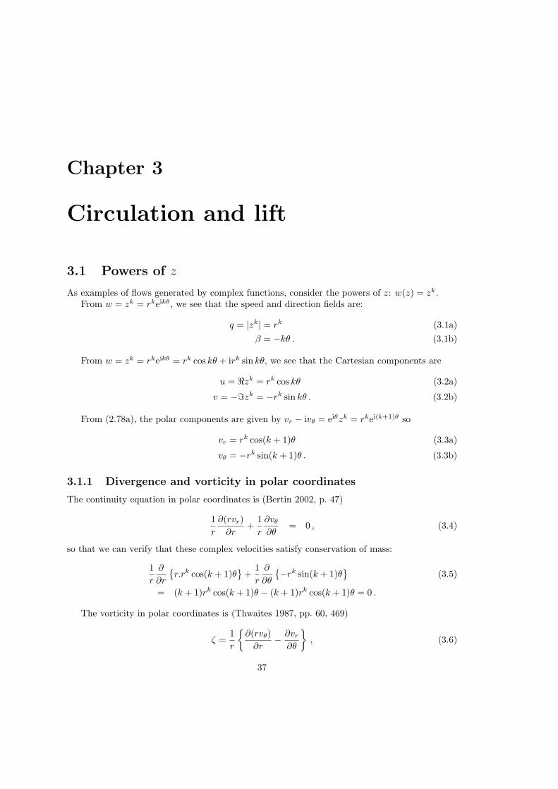
Chapter 3

Circulation and lift

3.1 Powers of z

As examples of flows generated by complex functions, consider the powers of z: w(z) = zk.From w = zk = rkeikθ, we see that the speed and direction fields are:

q = |zk| = rk (3.1a)

β = −kθ . (3.1b)

From w = zk = rkeikθ = rk cos kθ + irk sin kθ, we see that the Cartesian components are

u = ℜzk = rk cos kθ (3.2a)

v = −ℑzk = −rk sin kθ . (3.2b)

From (2.78a), the polar components are given by vr − ivθ = eiθzk = rkei(k+1)θ so

vr = rk cos(k + 1)θ (3.3a)

vθ = −rk sin(k + 1)θ . (3.3b)

3.1.1 Divergence and vorticity in polar coordinates

The continuity equation in polar coordinates is (Bertin 2002, p. 47)

1

r

∂(rvr)

∂r+

1

r

∂vθ

∂θ= 0 , (3.4)

so that we can verify that these complex velocities satisfy conservation of mass:

1

r

∂

∂r

{

r.rk cos(k + 1)θ}

+1

r

∂

∂θ

{

−rk sin(k + 1)θ}

(3.5)

= (k + 1)rk cos(k + 1)θ − (k + 1)rk cos(k + 1)θ = 0 .

The vorticity in polar coordinates is (Thwaites 1987, pp. 60, 469)

ζ =1

r

{

∂(rvθ)

∂r−∂vr

∂θ

}

, (3.6)

37

38 AERODYNAMICS I COURSE NOTES, 2006

so for w = zk,

ζ =1

r

{

∂(−rk+1 sin[k + 1]θ)

∂r−∂(rk cos[k + 1]θ)

∂θ

}

(3.7)

=1

r

{

−(k + 1)rk sin(k + 1)θ + (k + 1)rk sin(k + 1)θ}

= 0 . (3.8)

3.1.2 Complex potentials

The complex potential for the complex velocity w(z) = zk is

W (z) =

∫

zk dz =

{

(k + 1)−1zk+1 , (k 6= −1) ;

ln z , (k = −1) .(3.9)

Notice that the case w = z−1 is special. The logarithm of a complex number z satisfies

ln z = ln(

reiθ)

= ln r + ln(

eiθ)

= ln r + iθ . (3.10)

That is

ℜ(ln z) = ln |z| (3.11a)

ℑ(ln z) = arg z . (3.11b)

Thus for w = z−1,

φ = ln r (3.12a)

ψ = θ . (3.12b)

3.1.3 Examples

k = 1: corner flow

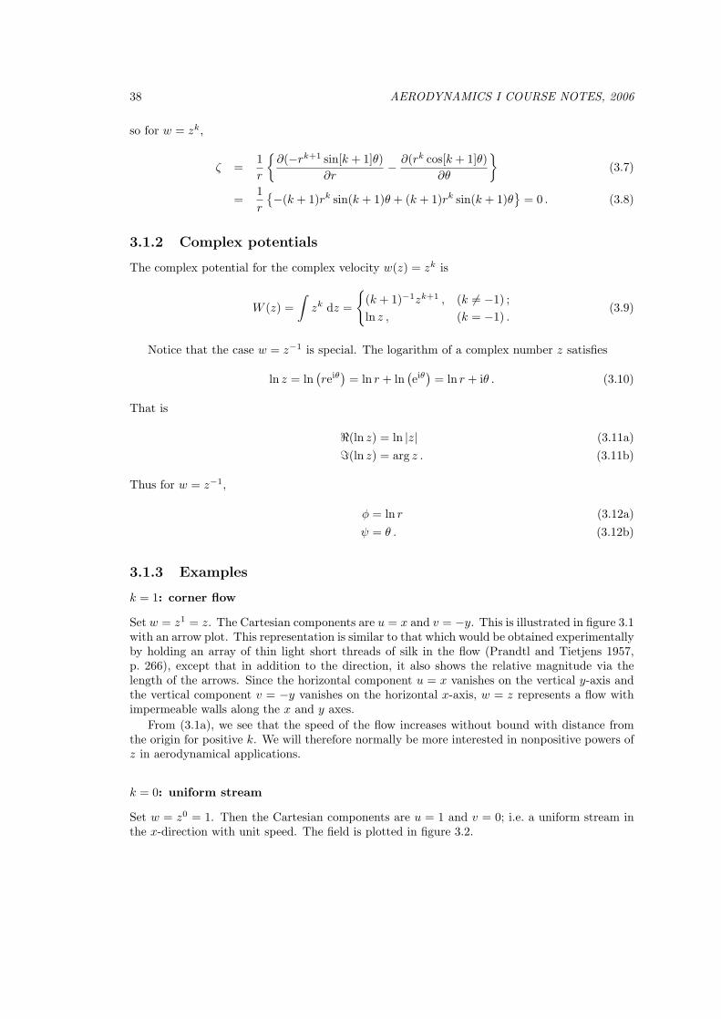
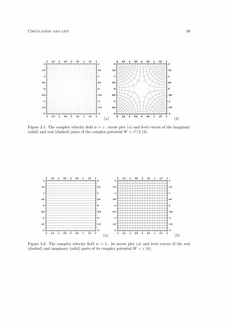
Set w = z1 = z. The Cartesian components are u = x and v = −y. This is illustrated in figure 3.1with an arrow plot. This representation is similar to that which would be obtained experimentallyby holding an array of thin light short threads of silk in the flow (Prandtl and Tietjens 1957,p. 266), except that in addition to the direction, it also shows the relative magnitude via thelength of the arrows. Since the horizontal component u = x vanishes on the vertical y-axis andthe vertical component v = −y vanishes on the horizontal x-axis, w = z represents a flow withimpermeable walls along the x and y axes.

From (3.1a), we see that the speed of the flow increases without bound with distance fromthe origin for positive k. We will therefore normally be more interested in nonpositive powers ofz in aerodynamical applications.

k = 0: uniform stream

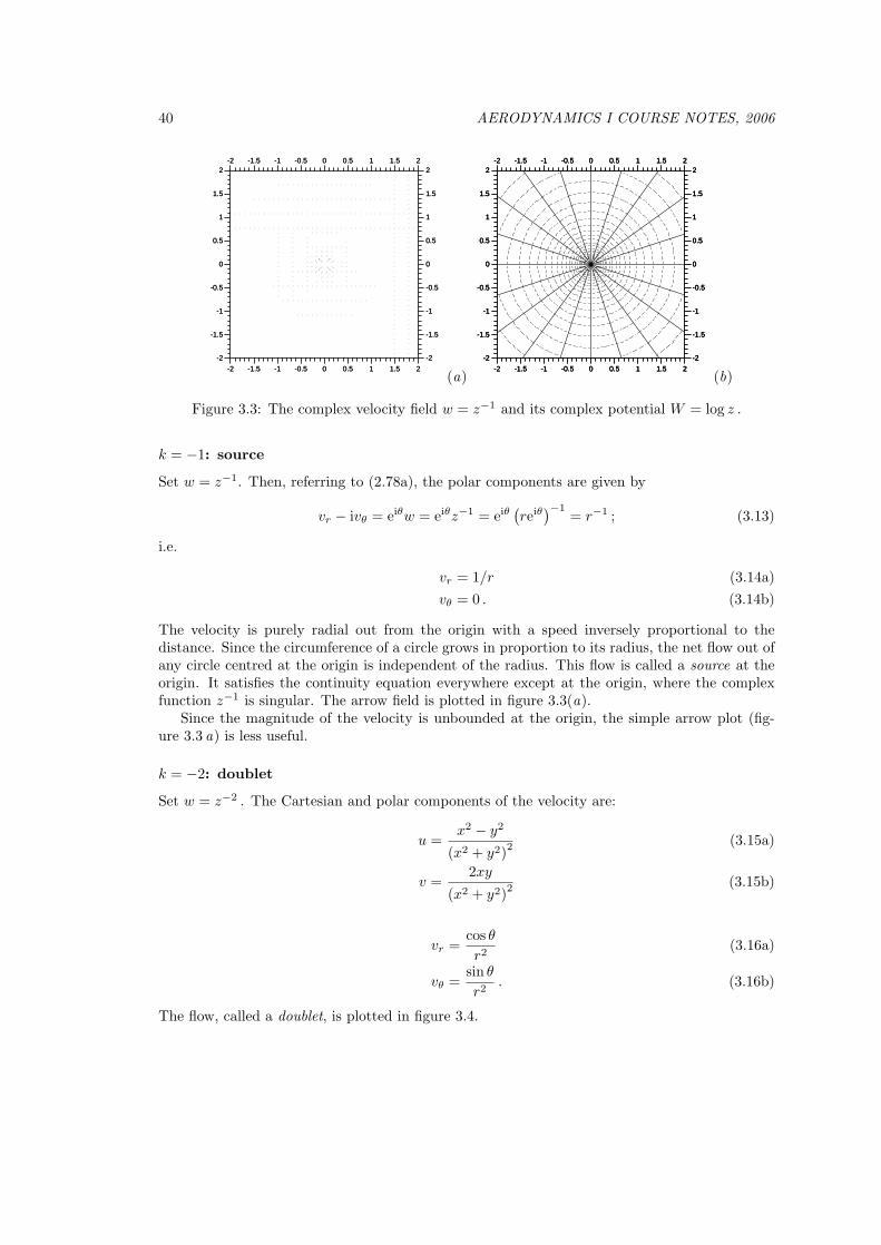
Set w = z0 = 1. Then the Cartesian components are u = 1 and v = 0; i.e. a uniform stream inthe x-direction with unit speed. The field is plotted in figure 3.2.

Circulation and lift 39

-2 -1.5 -1 -0.5 0 0.5 1 1.5 2

-2 -1.5 -1 -0.5 0 0.5 1 1.5 2

-2

-1.5

-1

-0.5

0

0.5

1

1.5

2

-2

-1.5

-1

-0.5

0

0.5

1

1.5

2

-2 -1.5 -1 -0.5 0 0.5 1 1.5 2

-2 -1.5 -1 -0.5 0 0.5 1 1.5 2

-2

-1.5

-1

-0.5

0

0.5

1

1.5

2

-2

-1.5

-1

-0.5

0

0.5

1

1.5

2

(a)-2 -1.5 -1 -0.5 0 0.5 1 1.5 2

-2 -1.5 -1 -0.5 0 0.5 1 1.5 2

-2

-1.5

-1

-0.5

0

0.5

1

1.5

2

-2

-1.5

-1

-0.5

0

0.5

1

1.5

2

-2 -1.5 -1 -0.5 0 0.5 1 1.5 2

-2 -1.5 -1 -0.5 0 0.5 1 1.5 2

-2

-1.5

-1

-0.5

0

0.5

1

1.5

2

-2

-1.5

-1

-0.5

0

0.5

1

1.5

2

-2 -1.5 -1 -0.5 0 0.5 1 1.5 2

-2 -1.5 -1 -0.5 0 0.5 1 1.5 2

-2

-1.5

-1

-0.5

0

0.5

1

1.5

2

-2

-1.5

-1

-0.5

0

0.5

1

1.5

2

(b)

Figure 3.1: The complex velocity field w = z : arrow plot (a) and level curves of the imaginary(solid) and real (dashed) parts of the complex potential W = z2/2 (b).

-2 -1.5 -1 -0.5 0 0.5 1 1.5 2

-2 -1.5 -1 -0.5 0 0.5 1 1.5 2

-2

-1.5

-1

-0.5

0

0.5

1

1.5

2

-2

-1.5

-1

-0.5

0

0.5

1

1.5

2

-2 -1.5 -1 -0.5 0 0.5 1 1.5 2

-2 -1.5 -1 -0.5 0 0.5 1 1.5 2

-2

-1.5

-1

-0.5

0

0.5

1

1.5

2

-2

-1.5

-1

-0.5

0

0.5

1

1.5

2

(a)-2 -1.5 -1 -0.5 0 0.5 1 1.5 2

-2 -1.5 -1 -0.5 0 0.5 1 1.5 2

-2

-1.5

-1

-0.5

0

0.5

1

1.5

2

-2

-1.5

-1

-0.5

0

0.5

1

1.5

2

-2 -1.5 -1 -0.5 0 0.5 1 1.5 2

-2 -1.5 -1 -0.5 0 0.5 1 1.5 2

-2

-1.5

-1

-0.5

0

0.5

1

1.5

2

-2

-1.5

-1

-0.5

0

0.5

1

1.5

2

(b)

Figure 3.2: The complex velocity field w = 1 : its arrow plot (a) and level curves of the real(dashed) and imaginary (solid) parts of its complex potential W = z (b).


-2 -1.5 -1 -0.5 0 0.5 1 1.5 2

-2 -1.5 -1 -0.5 0 0.5 1 1.5 2

-2

-1.5

-1

-0.5

0

0.5

1

1.5

2

-2

-1.5

-1

-0.5

0

0.5

1

1.5

2

-2 -1.5 -1 -0.5 0 0.5 1 1.5 2

-2 -1.5 -1 -0.5 0 0.5 1 1.5 2

-2

-1.5

-1

-0.5

0

0.5

1

1.5

2

-2

-1.5

-1

-0.5

0

0.5

1

1.5

2

(a)-2 -1.5 -1 -0.5 0 0.5 1 1.5 2

-2 -1.5 -1 -0.5 0 0.5 1 1.5 2

-2

-1.5

-1

-0.5

0

0.5

1

1.5

2

-2

-1.5

-1

-0.5

0

0.5

1

1.5

2

-2 -1.5 -1 -0.5 0 0.5 1 1.5 2

-2 -1.5 -1 -0.5 0 0.5 1 1.5 2

-2

-1.5

-1

-0.5

0

0.5

1

1.5

2

-2

-1.5

-1

-0.5

0

0.5

1

1.5

2

-2 -1.5 -1 -0.5 0 0.5 1 1.5 2

-2 -1.5 -1 -0.5 0 0.5 1 1.5 2

-2

-1.5

-1

-0.5

0

0.5

1

1.5

2

-2

-1.5

-1

-0.5

0

0.5

1

1.5

2

(b)

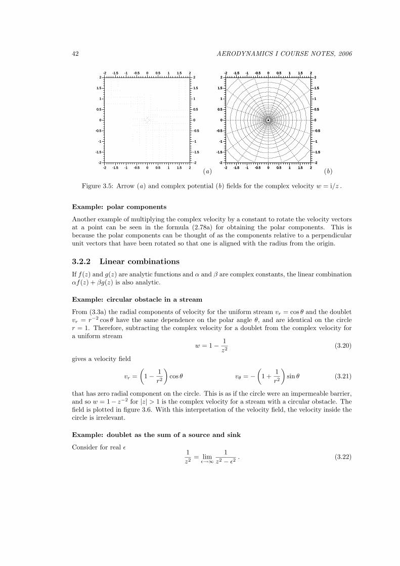
Figure 3.3: The complex velocity field w = z−1 and its complex potential W = log z .

k = −1: source

Set w = z−1. Then, referring to (2.78a), the polar components are given by

vr − ivθ = eiθw = eiθz−1 = eiθ(

reiθ)−1

= r−1 ; (3.13)

i.e.

vr = 1/r (3.14a)

vθ = 0 . (3.14b)

The velocity is purely radial out from the origin with a speed inversely proportional to thedistance. Since the circumference of a circle grows in proportion to its radius, the net flow out ofany circle centred at the origin is independent of the radius. This flow is called a source at theorigin. It satisfies the continuity equation everywhere except at the origin, where the complexfunction z−1 is singular. The arrow field is plotted in figure 3.3(a).

Since the magnitude of the velocity is unbounded at the origin, the simple arrow plot (fig-ure 3.3 a) is less useful.

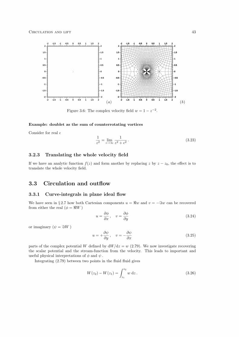
k = −2: doublet

Set w = z−2 . The Cartesian and polar components of the velocity are:

u =x2 − y2

(x2 + y2)2 (3.15a)

v =2xy

(x2 + y2)2 (3.15b)

vr =cos θ

r2(3.16a)

vθ =sin θ

r2. (3.16b)

The flow, called a doublet, is plotted in figure 3.4.


-2 -1.5 -1 -0.5 0 0.5 1 1.5 2

-2 -1.5 -1 -0.5 0 0.5 1 1.5 2

-2

-1.5

-1

-0.5

0

0.5

1

1.5

2

-2

-1.5

-1

-0.5

0

0.5

1

1.5

2

-2 -1.5 -1 -0.5 0 0.5 1 1.5 2

-2 -1.5 -1 -0.5 0 0.5 1 1.5 2

-2

-1.5

-1

-0.5

0

0.5

1

1.5

2

-2

-1.5

-1

-0.5

0

0.5

1

1.5

2

(a)-2 -1.5 -1 -0.5 0 0.5 1 1.5 2

-2 -1.5 -1 -0.5 0 0.5 1 1.5 2

-2

-1.5

-1

-0.5

0

0.5

1

1.5

2

-2

-1.5

-1

-0.5

0

0.5

1

1.5

2

-2 -1.5 -1 -0.5 0 0.5 1 1.5 2

-2 -1.5 -1 -0.5 0 0.5 1 1.5 2

-2

-1.5

-1

-0.5

0

0.5

1

1.5

2

-2

-1.5

-1

-0.5

0

0.5

1

1.5

2

-2 -1.5 -1 -0.5 0 0.5 1 1.5 2

-2 -1.5 -1 -0.5 0 0.5 1 1.5 2

-2

-1.5

-1

-0.5

0

0.5

1

1.5

2

-2

-1.5

-1

-0.5

0

0.5

1

1.5

2

(b)

Figure 3.4: The complex velocity field w = z−2 (a) and its complex potential W = −1/z (b) .

3.2 Modifying complex velocity fields

3.2.1 Multiplication by a complex constant

Say we have a complex velocity field w(z) expressed in polar form w = qe−iβ , where q is thespeed and β the angle to the positive x-axis. Multiplying an analytic function by a constantgives another analytic function. The velocity field obtained is

w′ =(

Aeiχ) (

qe−iβ)

= (Aq)e−i(β−χ) ,

so that the effect of multiplying by the complex constant Aeiχ is to change the speed to q′ = Aqand the direction to β′ = β − χ .

Thus, for example, noting that i = eiπ/2, multiplication by the imaginary unit i keeps thespeed the same but rotates the velocity vector at each point through a clockwise right-angle.

Example: uniform stream with arbitrary direction

The uniform horizontal (rightward) stream w(z) = 1 becomes, on multiplication by eiπ/2, w′ =iw = i, with components u′ = 0 and v′ = −1. This is a uniform vertical downward stream.

A uniform stream with speed q∞ and angle α is therefore obtained by multiplying the complexvelocity w = 1 by the complex constant q∞e−iα:

q∞e−iα = (q∞ cosα) − i (q∞ sinα) . (3.17)

Example: vortex

Since the velocity of a source is purely radial, multiplying its complex velocity z−1 by i rotatesthe velocity at each point through a right-angle to become purely azimuthal:

w = iz−1 = ir−1e−iθ (3.18)

vr − ivθ = eiθw = ir−1 , (3.19)

so vr = 0 and vθ = −1/r . This flow is called a vortex ; it is plotted in figure 3.5.


-2 -1.5 -1 -0.5 0 0.5 1 1.5 2

-2 -1.5 -1 -0.5 0 0.5 1 1.5 2

-2

-1.5

-1

-0.5

0

0.5

1

1.5

2

-2

-1.5

-1

-0.5

0

0.5

1

1.5

2

-2 -1.5 -1 -0.5 0 0.5 1 1.5 2

-2 -1.5 -1 -0.5 0 0.5 1 1.5 2

-2

-1.5

-1

-0.5

0

0.5

1

1.5

2

-2

-1.5

-1

-0.5

0

0.5

1

1.5

2

(a)-2 -1.5 -1 -0.5 0 0.5 1 1.5 2

-2 -1.5 -1 -0.5 0 0.5 1 1.5 2

-2

-1.5

-1

-0.5

0

0.5

1

1.5

2

-2

-1.5

-1

-0.5

0

0.5

1

1.5

2

-2 -1.5 -1 -0.5 0 0.5 1 1.5 2

-2 -1.5 -1 -0.5 0 0.5 1 1.5 2

-2

-1.5

-1

-0.5

0

0.5

1

1.5

2

-2

-1.5

-1

-0.5

0

0.5

1

1.5

2

-2 -1.5 -1 -0.5 0 0.5 1 1.5 2

-2 -1.5 -1 -0.5 0 0.5 1 1.5 2

-2

-1.5

-1

-0.5

0

0.5

1

1.5

2

-2

-1.5

-1

-0.5

0

0.5

1

1.5

2

(b)

Figure 3.5: Arrow (a) and complex potential (b) fields for the complex velocity w = i/z .

Example: polar components

Another example of multiplying the complex velocity by a constant to rotate the velocity vectorsat a point can be seen in the formula (2.78a) for obtaining the polar components. This isbecause the polar components can be thought of as the components relative to a perpendicularunit vectors that have been rotated so that one is aligned with the radius from the origin.

3.2.2 Linear combinations

If f(z) and g(z) are analytic functions and α and β are complex constants, the linear combinationαf(z) + βg(z) is also analytic.

Example: circular obstacle in a stream

From (3.3a) the radial components of velocity for the uniform stream vr = cos θ and the doubletvr = r−2 cos θ have the same dependence on the polar angle θ, and are identical on the circler = 1. Therefore, subtracting the complex velocity for a doublet from the complex velocity fora uniform stream

w = 1 −1

z2(3.20)

gives a velocity field

vr =

(

1 −1

r2

)

cos θ vθ = −

(

1 +1

r2

)

sin θ (3.21)

that has zero radial component on the circle. This is as if the circle were an impermeable barrier,and so w = 1− z−2 for |z| > 1 is the complex velocity for a stream with a circular obstacle. Thefield is plotted in figure 3.6. With this interpretation of the velocity field, the velocity inside thecircle is irrelevant.

Example: doublet as the sum of a source and sink

Consider for real ǫ1

z2= lim

ǫ→∞

1

z2 − ǫ2. (3.22)


-2 -1.5 -1 -0.5 0 0.5 1 1.5 2

-2 -1.5 -1 -0.5 0 0.5 1 1.5 2

-2

-1.5

-1

-0.5

0

0.5

1

1.5

2

-2

-1.5

-1

-0.5

0

0.5

1

1.5

2

-2 -1.5 -1 -0.5 0 0.5 1 1.5 2

-2 -1.5 -1 -0.5 0 0.5 1 1.5 2

-2

-1.5

-1

-0.5

0

0.5

1

1.5

2

-2

-1.5

-1

-0.5

0

0.5

1

1.5

2

(a)-2 -1.5 -1 -0.5 0 0.5 1 1.5 2

-2 -1.5 -1 -0.5 0 0.5 1 1.5 2

-2

-1.5

-1

-0.5

0

0.5

1

1.5

2

-2

-1.5

-1

-0.5

0

0.5

1

1.5

2

-2 -1.5 -1 -0.5 0 0.5 1 1.5 2

-2 -1.5 -1 -0.5 0 0.5 1 1.5 2

-2

-1.5

-1

-0.5

0

0.5

1

1.5

2

-2

-1.5

-1

-0.5

0

0.5

1

1.5

2

-2 -1.5 -1 -0.5 0 0.5 1 1.5 2

-2 -1.5 -1 -0.5 0 0.5 1 1.5 2

-2

-1.5

-1

-0.5

0

0.5

1

1.5

2

-2

-1.5

-1

-0.5

0

0.5

1

1.5

2

(b)

Figure 3.6: The complex velocity field w = 1 − z−2.

Example: doublet as the sum of counterrotating vortices

Consider for real ǫ1

z2= lim

ǫ→∞

1

z2 + ǫ2. (3.23)

3.2.3 Translating the whole velocity field

If we have an analytic function f(z) and form another by replacing z by z − z0, the effect is totranslate the whole velocity field.

3.3 Circulation and outflow

3.3.1 Curve-integrals in plane ideal flow

We have seen in § 2.7 how both Cartesian components u = ℜw and v = −ℑw can be recoveredfrom either the real (φ = ℜW )

u =∂φ

∂x, v =

∂φ

∂y(3.24)

or imaginary (ψ = ℑW )

u = +∂ψ

∂y, v = −

∂ψ

∂x(3.25)

parts of the complex potential W defined by dW/dz = w (2.79). We now investigate recoveringthe scalar potential and the stream-function from the velocity. This leads to important anduseful physical interpretations of φ and ψ .

Integrating (2.79) between two points in the fluid fluid gives

W (z2) −W (z1) =

∫ z2

z1

w dz . (3.26)


Expanding (3.26) into real and imaginary parts gives

φ(z2) − φ(z1) + i{ψ(z2) − ψ(z1)} =

∫ z2

z1

(u− iv) (dx+ idy)

=

∫ z2

z1

(u dx+ v dy) + i

∫ z2

z1

(u dy − v dx) . (3.27)

Now, as in the discussion of circulation in § 2.5.3,

u dx+ v dy = q · τ̂ ds ; (3.28)

i.e., the tangential component of velocity along an infinitesimal curve segment. And, as in thediscussion of conservation of mass in § 2.3,

u dy − v dx = q · n̂ ds ; (3.29)

i.e., the component of velocity at right-angles to the same segment (reckoned positive when thevelocity crosses the segment from left to right). Thus

φ(z2) − φ(z1) = ℜ

∫ z2

z1

w dz =

∫ z2

z1

q · τ̂ds (3.30a)

ψ(z2) − ψ(z1) = ℑ

∫ z2

z1

w dz =

∫ z2

z1

q · n̂ds . (3.30b)

In words, change in scalar potential along a curve through the flow field gives minus the circulationalong that curve, and the difference in the stream-function between two ends of the curve givesthe volumetric flow rate (per unit span) through the curve from left to right.

Also, formulae (3.30a)–(3.30b) can be used to determine or measure either φ or ψ , up to anarbitrary additive constant: the value at some reference point z1 .

3.3.2 Closed circuits

Now say we take the final point, z2 , of the curve to coincide with first point, z1 ; i.e. close thecurve to form a circuit C . Then

[W ]C =

∮

C

w dz (3.31)

where [W ]C means the jump in W as it moves around the circuit C . Of course, if W is asingle-valued function of z , [W ]C is necessarily zero for any circuit C ; however, we will see thatmultivalued complex potentials are also of interest in aerodynamics.

The real and imaginary parts involve the circulation ΓC around and outflow QC through thecircuit C,

[φ]C + i[ψ]C =

∮

C

(u dx+ v dy) + i

∮

C

(u dy − v dx) (3.32)

=

∮

C

q · τ̂ ds+ i

∮

C

q · n̂ ds (3.33)

≡ −ΓC + iQC . (3.34)


If the circuit C is filled with fluid, the circuit integrals can be replaced with integrals ofvorticity and divergence over the contained region R (see § 2.5.3 for the circulation and § 2.3 forthe outflow):

[φ]C = −ΓC =

∫∫

R

(

∂v

∂x−∂u

∂y

)

dx dy (3.35a)

[ψ]C = QC =

∫∫

R

(

∂u

∂x+∂v

∂y

)

dx dy . (3.35b)

If the velocity field in the region R is irrotational, the integrand in the integral for the circulationΓC vanishes, and if it’s divergence-free, the integrand in the integral for the outflow QC vanishes.

If the circuit is not filled with fluid in plane ideal flow, say, for example, because it enclosesan obstacle such as an aerofoil, then the integrals over R are meaningless, the circulation andoutflow need not vanish, and the complex potential might be multivalued. The same conclusionsapply if the circuit contains a singular point at which the velocity is undefined.

3.3.3 Example: powers of z and circles around the origin

Say we take w = Akzk = Akr

keikθ , where Ak is a complex constant, and let the circuit C be acircle of radius a , centred on the origin; i.e. on C , z = aeiθ . Then around the circuit,

dz = d(aeiθ) = aieiθ dθ (3.36)

with θ going from 0 to 2π , and the integral around the circuit is

∮

C

w dz = Ak

∫ 2π

0

akeikθiaeiθ dθ (3.37)

= iak+1Ak

∫ 2π

0

ei(k+1)θdθ . (3.38)

Now if k 6= −1, this is

∮

C

Akzk dz = iak+1Ak

[

ei(k+1)θ

i(k + 1)

]2π

0

(3.39)

= 0 , (3.40)

since eiθ = cos θ + i sin θ is periodic in θ with period 2π.

For the special case k = −1, though, we have

∮

C

A−1

zdz = ia0A−1

∫ 2π

0

ei(0)θdθ (3.41)

= iA−1

∫ 2π

0

dθ (3.42)

= 2πiA−1 . (3.43)

Notice that this result is independent of the radius of the circle used for integration. In fact,though not proven here, the circulation Γ and outflow Q are both independent of the shape ofthe circuit too, so long as the circuit encloses the same obstacles and singularities.


In summary, for w = Akzk , Γ = Q = 0 for k 6= −1 . For w = A−1/z , Γ = 2πℑA−1 and

Q = 2πℜA−1 . For this reason we usually represent a point source at the origin as

wsource =Q

2πz(3.44)

and a point vortex as

wvortex = iΓ

2πz, (3.45)

and call Q and Γ the strengths of the source and vortex. For Q < 0 , we call the source a sink.The results obtained here correspond to the fact that the complex potentials for w = Akz

k

are, as in § 3.1.2,

W =

∫

Akzk dz =

{

Ak(k + 1)−1zk+1 , (k 6= −1) ;

A−1 ln z , (k = −1) ,(3.46)

i.e. all single-valued except for when k = −1 .

3.4 More on the scalar potential and stream-function

3.4.1 The scalar potential and irrotational flow

We have seen that in an ideal flow, the difference in the scalar potential between two points isequal to minus the circulation along a path though the fluid joining them. In general, any planevelocity field derived from a scalar function φ by the operations

u =∂φ

∂x, v =

∂φ

∂y(3.47)

will be irrotational, since

ζ ≡∂v

∂x−∂u

∂y=

∂2φ

∂x∂y−

∂2φ

∂y∂x= 0 . (3.48)

On the other hand, if the scalar potential isn’t the real part of an analytic function, the derivedvelocity field needn’t be divergence-free; the condition ∇ · q = 0 (2.3) becomes

∂2φ

∂x2+∂2φ

∂y2= 0 . (3.49)

This second-order linear partial differential equation is called Laplace’s equation, and is oftenwritten concisely as

∇2φ = 0 . (3.50)

3.4.2 The stream-function and divergence-free flow

If a velocity field is derived from a scalar function ψ by

u = +∂ψ

∂y, v = −

∂ψ

∂x, (3.51)

it will automatically be divergence-free since

∂u

∂x+∂v

∂y=

∂2ψ

∂x∂y−

∂2ψ

∂y∂x= 0 . (3.52)


On the other hand, it needn’t be irrotational: the condition that it is is

ζ =∂v

∂x−∂u

∂y= −

∂2ψ

∂x2−∂2ψ

∂y2≡ −∇2ψ = 0 . (3.53)

Thus, velocity fields derived from an analytic complex velocity are automatically divergence-free and irrotational, those derived from a scalar potential are irrotational, and those from astream-function divergence-free. Scalar potentials or stream-functions can be used for ideal flow,but only if they satisfy Laplace’s equation (3.50).

For more general, nonideal, kinds of flow, there is no complex velocity, and these representa-tions can be useful. Thus, the scalar potential can be used for irrotational flow of compressiblefluids (for which generally the divergence is nonzero), and the stream-function can be used forviscous flow of incompressible fluids (for which vorticity is generated at the flow boundaries).

3.5 Lift

In this section, we derive an expression for the aerodynamic force per unit span on an impermeableobject in a plane ideal flow in terms of the complex velocity. We then show that the drag alwaysvanishes while the lift is proportional to the circulation around the object.

3.5.1 Blasius’s theorem

The Cartesian components of the aerodynamic force per unit span on an obstacle with contourC are given by (2.19)–(2.20). From them, form the complex quantity

ax − iay = −

∮

C

p (dy + i dx) = −i

∮

C

p dz∗ (3.54)

and use Bernoulli’s equation for ideal flow (2.45), dropping the constant terms which integrateto zero,

ax − iay = −i

∮

C

(

p∞ +ρq2∞2

−ρq2

2

)

dz∗ (3.55)

=iρ

2

∮

C

q2 dz∗ (3.56)

=iρ

2

∮

C

ww∗ dz∗ . (3.57)

Now

w∗ dz∗ = (w dz)∗ = dW ∗ = dφ− i dψ (3.58)

but dψ = 0 along the outline of an impermeable obstacle, so we can replace dW ∗ with its complexconjugate dφ+ i dψ = dW ≡ w dz and

ax − iay =iρ

2

∮

C

w2 dz (3.59)

which is Blasius’s Theorem.

References: Glauert (1947, p. 81), Milne-Thomson (1973, p. 89).


3.5.2 The Kutta–Joukowsky theorem

Now say, for example, the flow is composed of a uniform stream with speed q∞ and incidence αand a vortex of strength Γ ; i.e.

w = q∞e−iα + iΓ

2πz. (3.60)

Then

w2 = q2∞e−i2α + iq∞Γ

πze−iα −

Γ 2

4π2z2

, (3.61)

and using the results on the circuit integrals of powers of z from § 3.3.3∮

C

w2 dz = 2πi ×

(

iq∞Γ

π

e−iα

)

(3.62)

= −2q∞Γ e−iα . (3.63)

Blasius’s theorem (3.59) then gives

ax − iay = −iρq∞Γ e−iα . (3.64)

Since the drag is measured in the direction of the airstream (α ) and the lift is measured a right-angle anticlockwise from the drag (α+ π/2 ), we have (as in § 2.6.2 for velocity components)

ℓ− i(−d) = ℓ+ id =ei(α+π/2)(ax − iay) = ρq∞Γ ; (3.65)

i.e.

ℓ = ρq∞Γ (3.66a)

d = 0 . (3.66b)

If the vortex is clockwise Γ > 0 and the lift is positive (ρ and q∞ are always positive).These two results constitute the Kutta–Joukowsky Theorem, which actually holds for any flow

over any aerofoil and is perhaps the most important result in two-dimensional aerodynamics. Itmeans that instead of having to calculate the aerodynamic force by integrating contributionsfrom stresses around the surface, we can just calculate the circulation and use (3.66).

The Kutta–Joukowsky Theorem is easily verified for plane ideal flow over a circular cylinder.More general flows than (3.60) could be considered by adding more terms to the series. Terms

of the form zk with positive k should be excluded, however, as they imply speeds increasingwithout bound in the far field (q ∼ |z|k ). Terms of the form zk with k = −2,−3, . . . on the otherhand all only produce terms like zm with m 6 −2 in w2 , and none of these contribute to thecontour integral: all zm terms vanish except those for m = −1 .

The interpretation of the theorem is straightforward. We know that the pressure is related tothe kinetic energy of the fluid (i.e. the square of the velocity) by Bernoulli’s equation, and so itis pairwise products of velocities that will be of interest. Of all possible pairs of velocities of thetype zk , the only combination giving an average speed difference between the upper and lowersurfaces is one varying like cos θ or sin θ or e±iθ , not einθ for any n 6= ±1 . If the velocities arerestricted to have k 6 0 (by the requirement of bounded velocity in the far field) this leaves onlythe possibility 0−1 = −1 or −1+0 = −1, the uniform stream–vortex pairing. In this pairing, thevortex on one side reinforces the stream and on the other retards it, and it is this that generatesthe net difference in speeds, kinetic energies, and pressures, and therefore generates the net lift.On the other hand, there exists no such mechanism for the generation of drag by plane idealflow.

References: Glauert (1947, p. 82), Prandtl and Tietjens (1957, pp. 161–166), Abbott and vonDoenhoff (1959, ch. 3), Milne-Thomson (1973, p. 91), Kuethe and Chow (1998, p. 107), Anderson(2001, pp. 238–239), Bertin (2002, p. 90), Moran (2003, p. 88).

Circulation and Lift

Documents

Transcript of Circulation and Lift