KARL PEARSON(1857-1936)

British mathematician, ‘father’ of modern statistics and a pioneer of eugenics!

(Pearson’s)

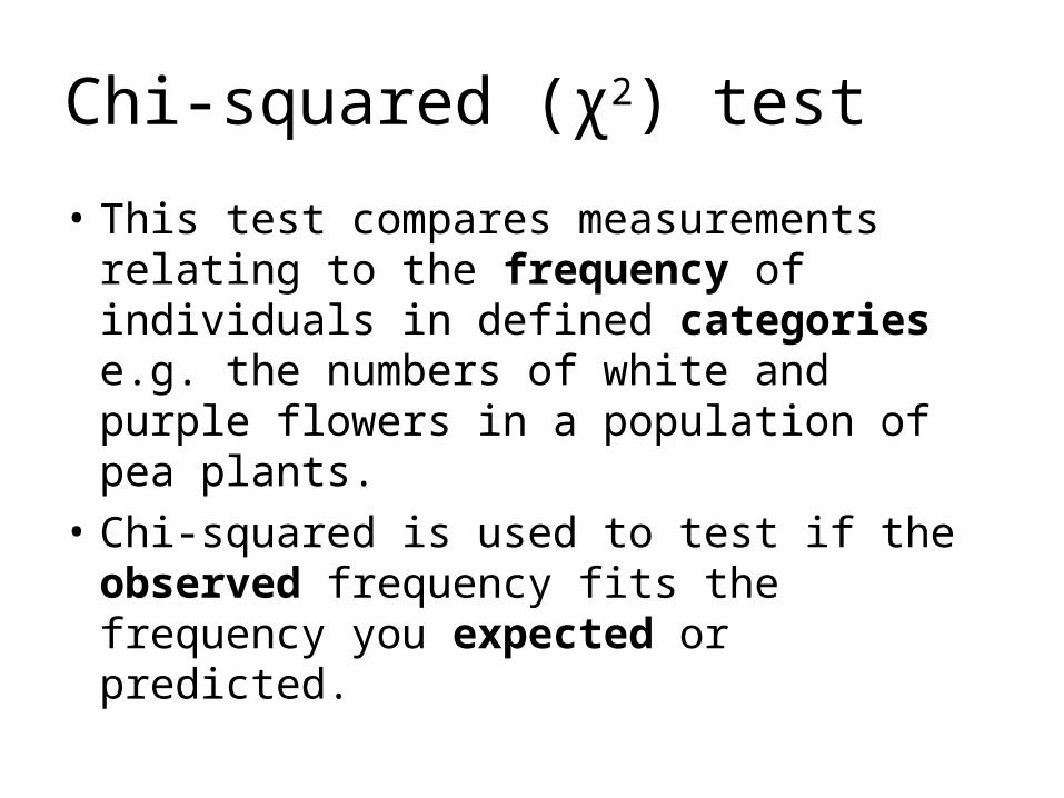
Chi-squared (χ2) test

• This test compares measurements relating to the frequency of individuals in defined categories e.g. the numbers of white and purple flowers in a population of pea plants.

• Chi-squared is used to test if the observed frequency fits the frequency you expected or predicted.

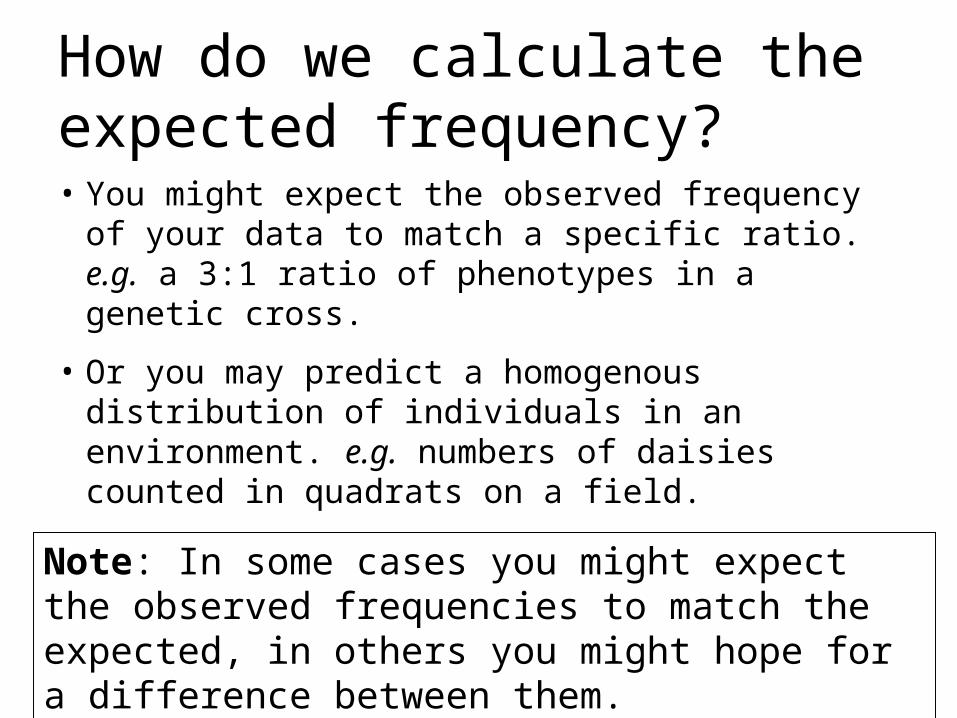
How do we calculate the expected frequency?• You might expect the observed frequency of

your data to match a specific ratio. e.g. a 3:1 ratio of phenotypes in a genetic cross.

• Or you may predict a homogenous distribution of individuals in an environment. e.g. numbers of daisies counted in quadrats on a field.

Note: In some cases you might expect the observed frequencies to match the expected, in others you might hope for a difference between them.

Example 1: GENETICS

Comparing the observed frequency of different types of maize grains with the expected ratio calculated using a Punnett square.

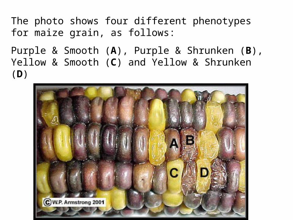
The photo shows four different phenotypes for maize grain, as follows:

Purple & Smooth (A), Purple & Shrunken (B), Yellow & Smooth (C) and Yellow & Shrunken (D)

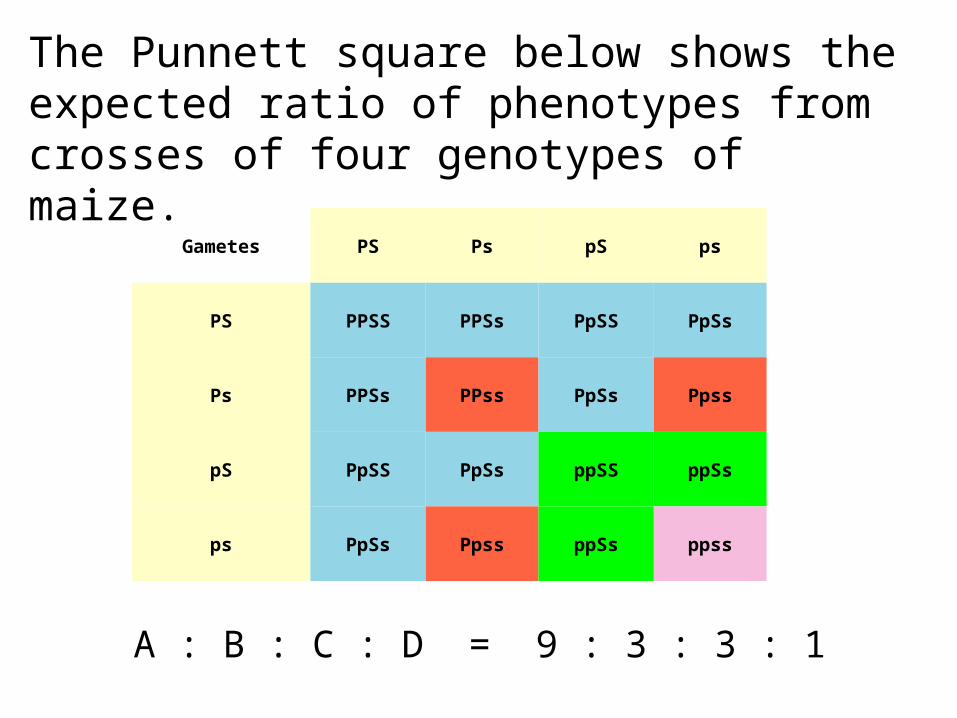
Gametes PS Ps pS ps

PS PPSS PPSs PpSS PpSs

Ps PPSs PPss PpSs Ppss

pS PpSS PpSs ppSS ppSs

ps PpSs Ppss ppSs ppss

The Punnett square below shows the expected ratio of phenotypes from crosses of four genotypes of maize.

A : B : C : D = 9 : 3 : 3 : 1

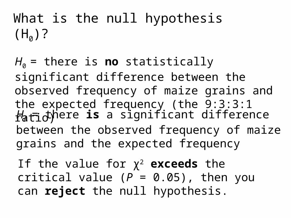
H0 = there is no statistically significant difference between the observed frequency of maize grains and the expected frequency (the 9:3:3:1 ratio)

HA = there is a significant difference between the observed frequency of maize grains and the expected frequency

If the value for χ2 exceeds the critical value (P = 0.05), then you can reject the null hypothesis.

What is the null hypothesis (H0)?

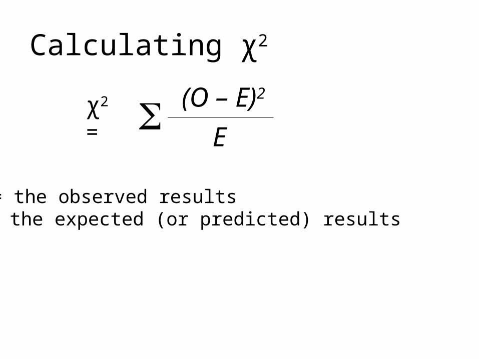
Calculating χ2

χ2 = (O – E)2

E

O = the observed resultsE = the expected (or predicted) results

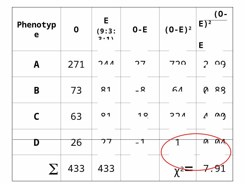
Phenotype O E(9:3:3:1)

O-E (O-E)2 (O-E)2

E

A 271 244 27 729 2.99

B 73 81 -8 64 0.88

C 63 81 -18 324 4.00

D 26 27 -1 1 0.04

433 433 χ2= 7.91

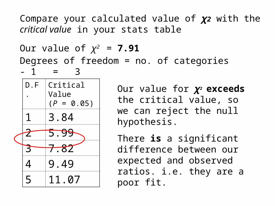
Compare your calculated value of χ2 with the critical value in your stats table

Our value of χ2 = 7.91Degrees of freedom = no. of categories - 1 = 3

D.F. Critical Value (P = 0.05)

1 3.842 5.993 7.824 9.495 11.07

Our value for χ2 exceeds the critical value, so we can reject the null hypothesis.

There is a significant difference between our expected and observed ratios. i.e. they are a poor fit.

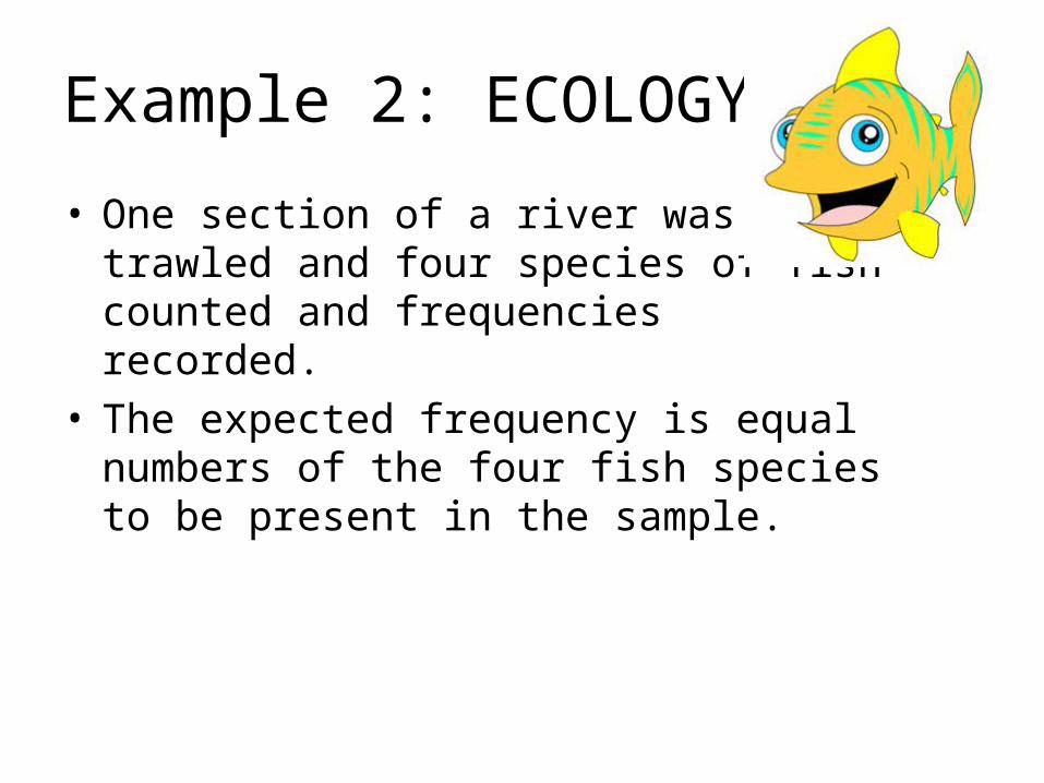
Example 2: ECOLOGY

• One section of a river was trawled and four species of fish counted and frequencies recorded.

• The expected frequency is equal numbers of the four fish species to be present in the sample.

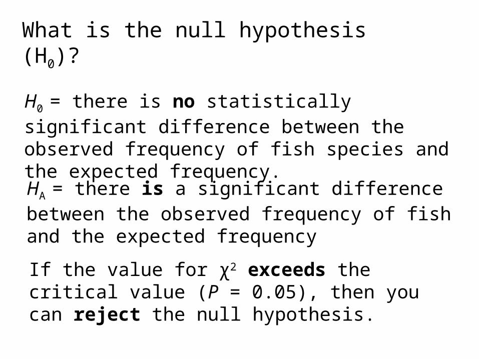
H0 = there is no statistically significant difference between the observed frequency of fish species and the expected frequency.

HA = there is a significant difference between the observed frequency of fish and the expected frequency

If the value for χ2 exceeds the critical value (P = 0.05), then you can reject the null hypothesis.

What is the null hypothesis (H0)?

Calculating χ2

χ2 = (O – E)2

E

O = the observed resultsE = the expected (or predicted) results

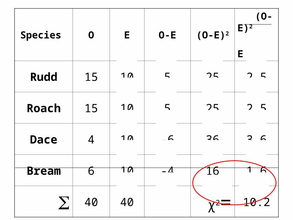
Species O E O-E (O-E)2 (O-E)2

E

Rudd 15 10 5 25 2.5

Roach 15 10 5 25 2.5

Dace 4 10 -6 36 3.6

Bream 6 10 -4 16 1.6

40 40 χ2= 10.2

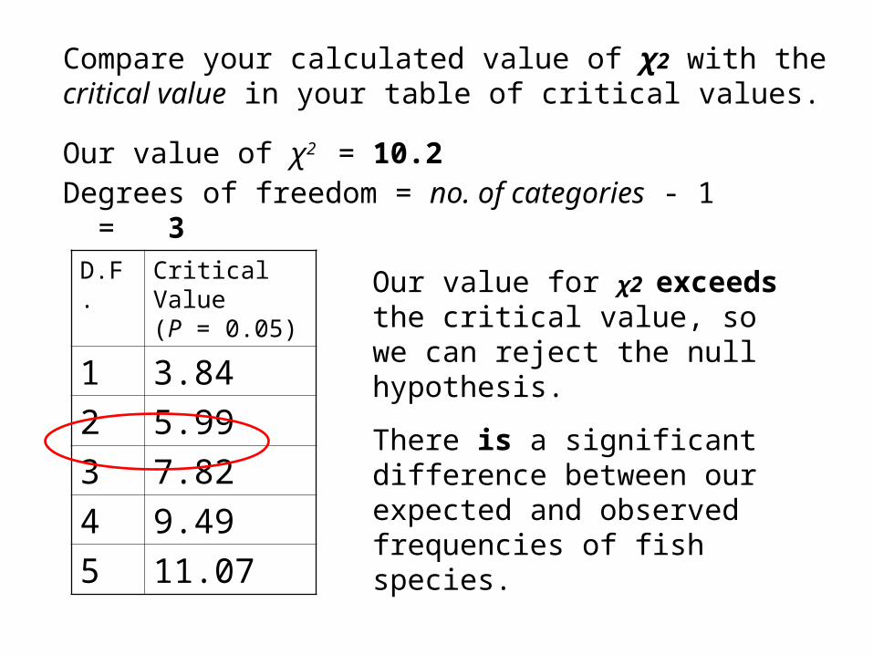
Compare your calculated value of χ2 with the critical value in your table of critical values.

Our value of χ2 = 10.2Degrees of freedom = no. of categories - 1 = 3

D.F. Critical Value (P = 0.05)

1 3.842 5.993 7.824 9.495 11.07

Our value for χ2 exceeds the critical value, so we can reject the null hypothesis.

There is a significant difference between our expected and observed frequencies of fish species.

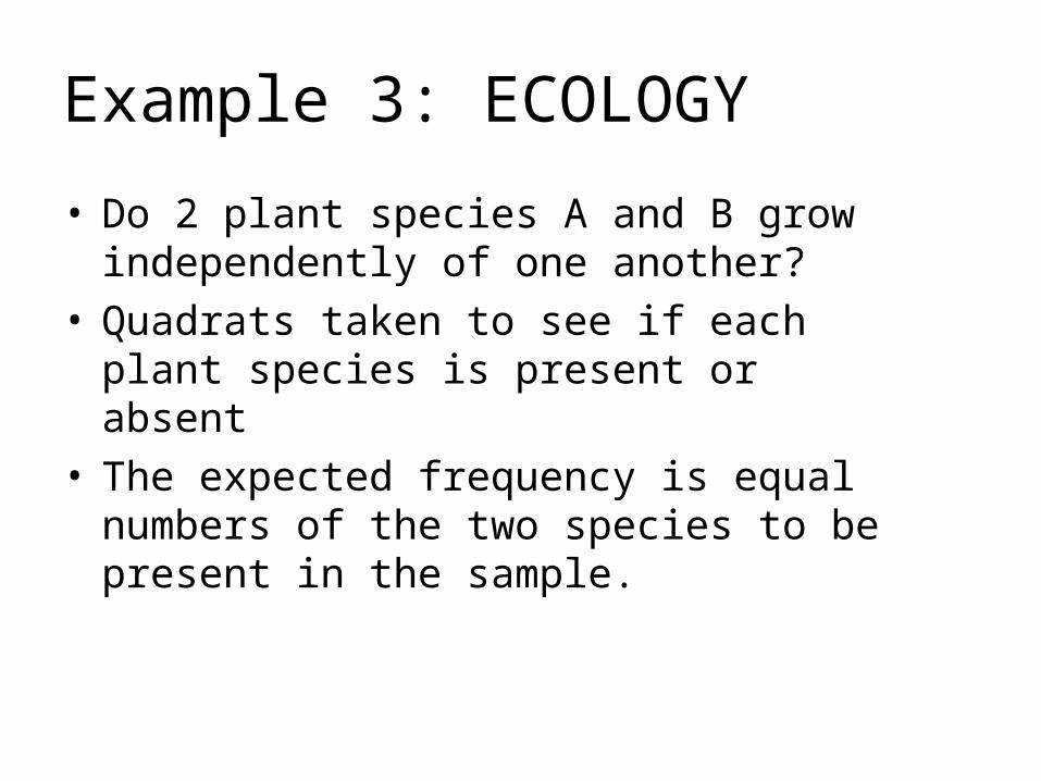
Example 3: ECOLOGY

• Do 2 plant species A and B grow independently of one another?

• Quadrats taken to see if each plant species is present or absent

• The expected frequency is equal numbers of the two species to be present in the sample.

Observed valuesSpecies A

Present Absent Totals

Specis BPresent 111 9 120

Absent 71 43 114

182 52 234

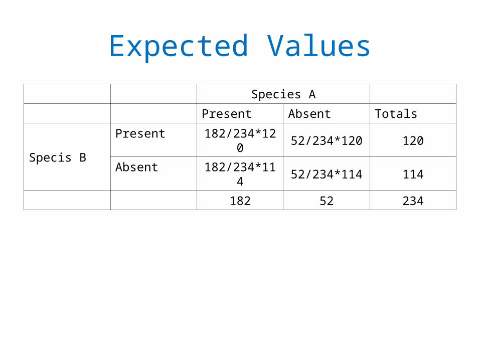
Expected ValuesSpecies A

Present Absent Totals

Specis BPresent 182/234*120 52/234*120 120

Absent 182/234*114 52/234*114 114

182 52 234

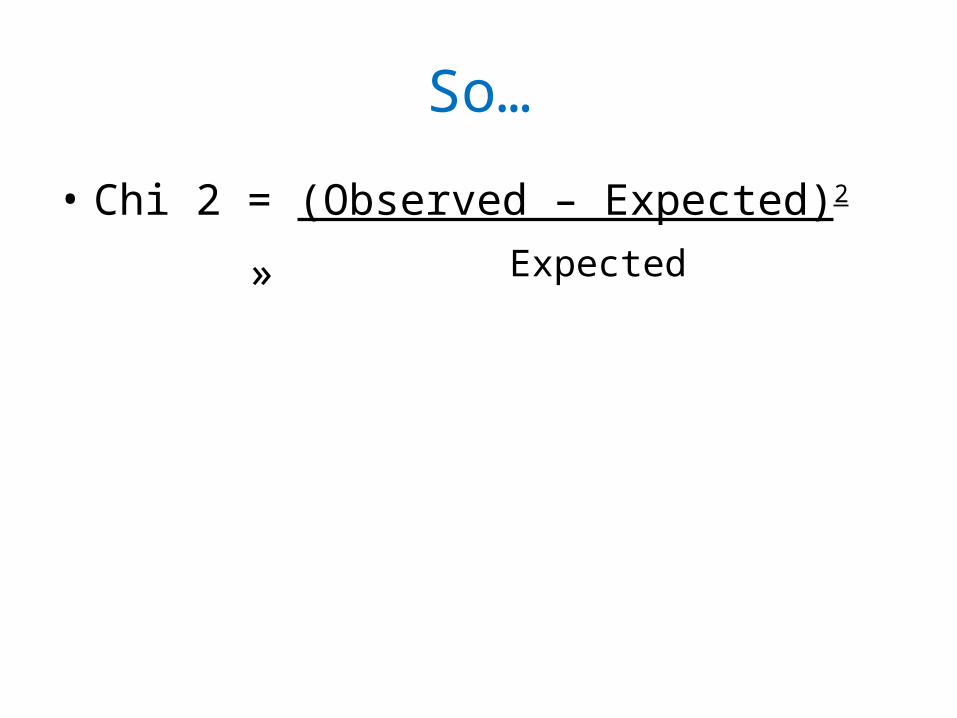
So…

• Chi 2 = (Observed – Expected)2

» Expected

• Null hypothesis:

• If the plants grow independently of each other there should be no statistically significant difference in the number of species A seen when B is present as when it is absent! And vice versa

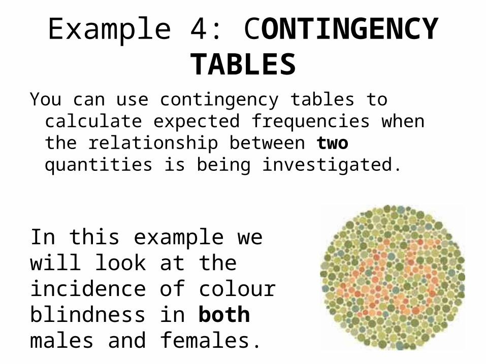
Example 4: CONTINGENCY TABLES

You can use contingency tables to calculate expected frequencies when the relationship between two quantities is being investigated.

In this example we will look at the incidence of colour blindness in both males and females.

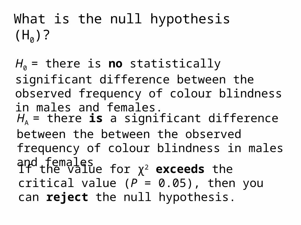
H0 = there is no statistically significant difference between the observed frequency of colour blindness in males and females.

HA = there is a significant difference between the between the observed frequency of colour blindness in males and females

If the value for χ2 exceeds the critical value (P = 0.05), then you can reject the null hypothesis.

What is the null hypothesis (H0)?

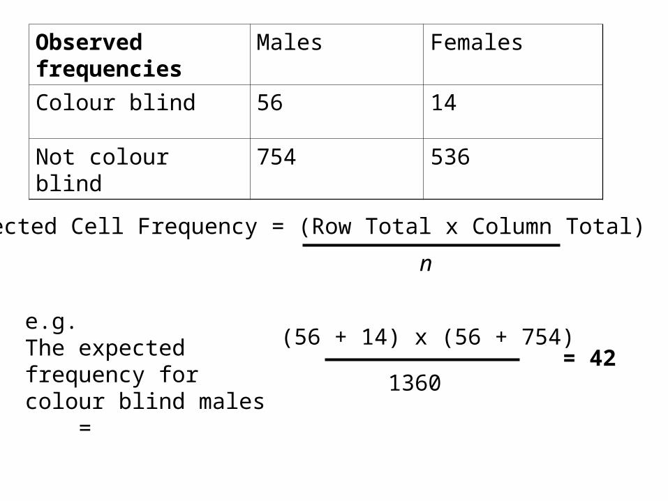
Observed frequencies Males Females

Colour blind 56 14

Not colour blind 754 536

e.g.The expected frequency for colour blind males =

(56 + 14) x (56 + 754)

1360= 42

Expected Cell Frequency = (Row Total x Column Total)

n

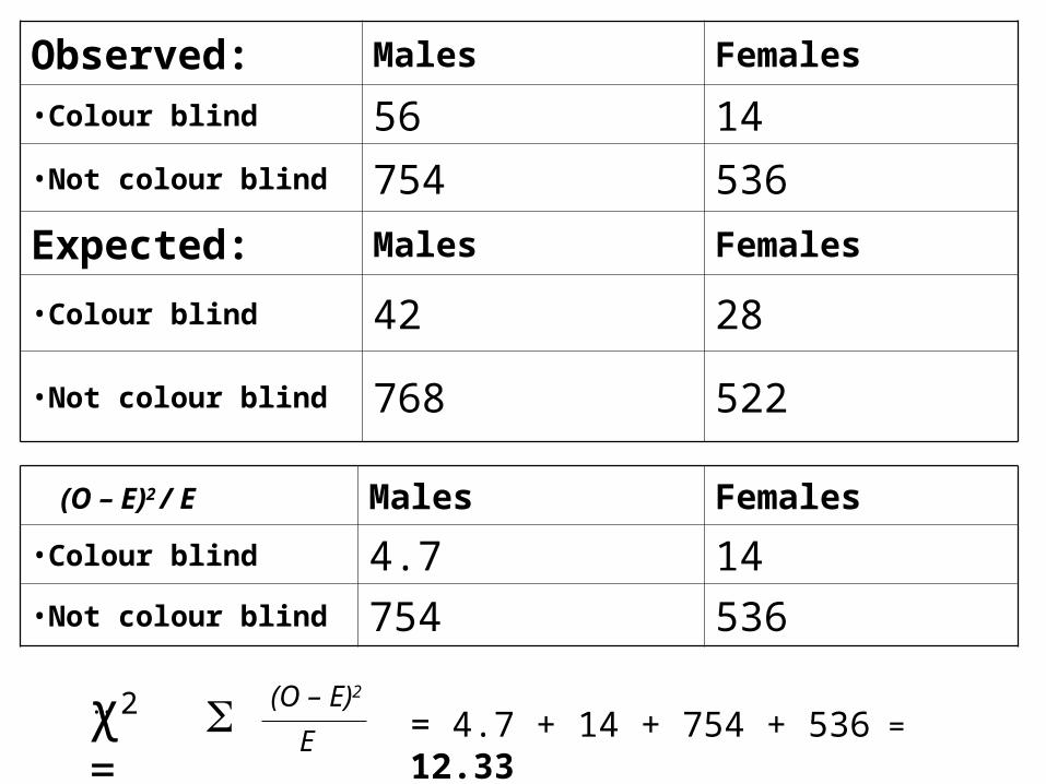
Observed: Males Females

•Colour blind 56 14•Not colour blind 754 536

Expected: Males Females

•Colour blind 42 28

•Not colour blind 768 522

Males Females

•Colour blind 4.7 14•Not colour blind 754 536

χ2 =… (O – E)2

E = 4.7 + 14 + 754 + 536 = 12.33

(O – E)2 / E

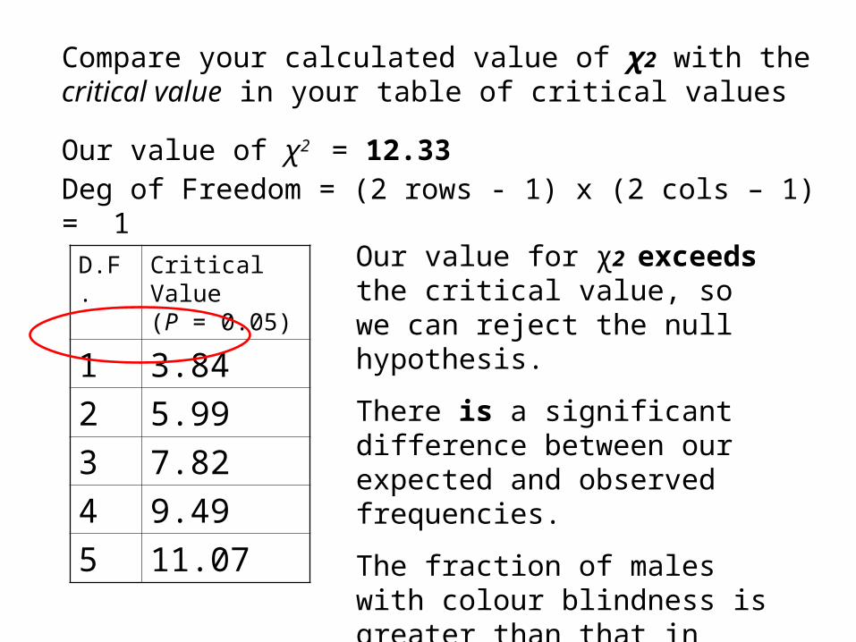
Compare your calculated value of χ2 with the critical value in your table of critical values

Our value of χ2 = 12.33Deg of Freedom = (2 rows - 1) x (2 cols – 1) = 1

D.F. Critical Value (P = 0.05)

1 3.842 5.993 7.824 9.495 11.07

Our value for χ2 exceeds the critical value, so we can reject the null hypothesis.

There is a significant difference between our expected and observed frequencies.

The fraction of males with colour blindness is greater than that in females. The difference cannot be attributed to chance alone.