χChek RC2 User Manual - University of Torontoarie/xchek/xchek_user_manual.pdf · 4.1 Loading a...

χChek RC2 User Manual

Documentation maintained byJocelyn Simmonds and Arie Gurfinkel

[email protected] of Computer Science

40 St George StreetUniversity of Toronto

Toronto, Ontario, CanadaM5S 2E4

This document is part of the distribution package of theχChek model checker.Copyright c©2002 – 2007 by University of Toronto

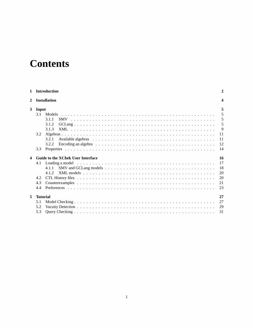
Contents

1 Introduction 2

2 Installation 4

3 Input 53.1 Models . . . . . . . . . . . . . . . . . . . . . . . . . . . . . . . . . . . . . . . . . .. . . . . . . . 5

3.1.1 SMV . . . . . . . . . . . . . . . . . . . . . . . . . . . . . . . . . . . . . . . . . . .. . . . 53.1.2 GCLang . . . . . . . . . . . . . . . . . . . . . . . . . . . . . . . . . . . . . . . .. . . . . . 53.1.3 XML . . . . . . . . . . . . . . . . . . . . . . . . . . . . . . . . . . . . . . . . . . .. . . . 9

3.2 Algebras . . . . . . . . . . . . . . . . . . . . . . . . . . . . . . . . . . . . . . . .. . . . . . . . . . 113.2.1 Available algebras . . . . . . . . . . . . . . . . . . . . . . . . . . . . .. . . . . . . . . . . 113.2.2 Encoding an algebra . . . . . . . . . . . . . . . . . . . . . . . . . . . . .. . . . . . . . . . 12

3.3 Properties . . . . . . . . . . . . . . . . . . . . . . . . . . . . . . . . . . . . . .. . . . . . . . . . . 14

4 Guide to the XChek User Interface 164.1 Loading a model . . . . . . . . . . . . . . . . . . . . . . . . . . . . . . . . . . .. . . . . . . . . . 17

4.1.1 SMV and GCLang models . . . . . . . . . . . . . . . . . . . . . . . . . . . .. . . . . . . . 184.1.2 XML models . . . . . . . . . . . . . . . . . . . . . . . . . . . . . . . . . . . . .. . . . . . 20

4.2 CTL History files . . . . . . . . . . . . . . . . . . . . . . . . . . . . . . . . . .. . . . . . . . . . . 204.3 Counterexamples . . . . . . . . . . . . . . . . . . . . . . . . . . . . . . . . .. . . . . . . . . . . . 214.4 Preferences . . . . . . . . . . . . . . . . . . . . . . . . . . . . . . . . . . . . .. . . . . . . . . . . 23

5 Tutorial 275.1 Model Checking . . . . . . . . . . . . . . . . . . . . . . . . . . . . . . . . . . .. . . . . . . . . . . 275.2 Vacuity Detection . . . . . . . . . . . . . . . . . . . . . . . . . . . . . . . .. . . . . . . . . . . . . 295.3 Query Checking . . . . . . . . . . . . . . . . . . . . . . . . . . . . . . . . . . .. . . . . . . . . . . 31

1

Chapter 1

Introduction

χChek is a multi-valued symbolic model checker [CDG02]. It isa generalization of an existing symbolic modelchecking algorithm to an algorithm for a multi-valued extension of CTL (χCTL). Given a system and aχCTL property,χChek returns thedegreeto which the system satisfies the property. By multi-valued logic we mean a logic whosevalues form afinite quasi-boolean distributive lattice. The meet and join operations of the lattice are interpretedasthe logicalandandor, respectively. The negation is given by a lattice dual-automorphism with period 2, ensuring thepreservation of involution of negation (¬¬a = a) and De Morgan laws.

Multi-valued model checking generalizes classical model checking and is useful for analyzing models where thereis uncertainty (e.g. missing information) or inconsistency (e.g. disagreement between different views). Multi-valuedlogics support the explicit modeling of uncertainty and disagreement by providing additional truth values in the logic.χChek works for any member of a large class of multi-valued logics. It’s model of computations is based on ageneralization of Kripke structures, where both atomic propositions and transitions between states may take any of thetruth values of a given multi-valued logic. Properties are expressed inχCTL, a multi-valued extension of the temporallogic CTL.

Additional information about the algorithms and the data structures used byχChek is available in [Gur02, CDEG03,CGD+06]

χChek is distributed under a FreeBSD license. For the terms ofthis license, seehttp://www.freebsd.org/copyright/freebsd-license.html .

The main features ofχChek are the following:

• Multi-valued logics: 2-valued, 3-valued, upset, 4-valueddisagreements, etc. Users can define their own logics.

• Multiple model formats: reads SMV and GCLang models. Multi-valued models are specified in XML.

• Proof-like counterexamples: proof rules are used to generate counterexamples. Counterexamples can be gener-ated statically or dynamically, and various viewers are available.

This document is structured as follows:

• Chapter 2: Installation

• Chapter 3: Input (models, algebras and properties)

• Chapter 4: Guide to theχChek User Interface (loading models, CTL history files, counterexample viewers andpreferences)

• Chapter 5: Tutorial (model checking, vacuity detection andquery checking)

Known bugs and limitations:

• χChek sometimes runs out of memory when statically computinga counterexample.

2

• χChek is a “best-effort” implementation. We recommend restarting χChek before loading a new model.

Collaborators:Marsha Chechik, Benet Devereux, Steve Easterbrook, Arie Gurfinkel, Kelvin Ku, Shiva Nejati, Viktor Petrovykh,

Jocelyn Simmonds, Rohit Talati, Anya Tafliovich, Christopher Thompson-Walsh, Kapil Shukla, and Xin (John) Ma.

3

Chapter 2

Installation

Prerequisites

• Linux-based OS (Fedora Core 4-7, and Ubuntu 7 are known to work).

• Java SE 6.

• Apache ant version≥ 1.6.5 (only for compilation)

Installation

1. DownloadχChek distribution archive.

2. Extract theχChek archive to create a directoryxchek , with the following structure:

build.xml χChek ant buildfile.

bin scripts for runningχChek.

doc documentation. Includes JavaDoc API and this doucment

jsrc the source code

lib bindings to C libraries

ext 3rd-party Java libraries

examples example models and properties

3. (Optional) Recompile by runningant

4. Runbin/xc to executeχChek.

NotesThe amount of memory given toχChek is controlled by setting environment variablesMEMORYMIN andMEMORYMAX.

For example, in bash,

# MEMORYMIN=512m MEMORYMAX=1024m ./bin/xc

will start χChek with 512MB of available RAM, and will allow the process to use up to 1024MB.

4

Chapter 3

Input

This chapter describes the syntax of model-specification languages, the syntax of algebra (multi-valued logic) specifi-cations, and the syntax of temporal logic properties.

χChek supports models specified in either a simplified versionof the SMV [CCG+02] modeling language, orthe Guarded Command Language (GCLang). Arbitrary multi-valued models are specified in XML, by explicitlydescribing the model’s Kripke structure (i.e., states and transitions). These XML files also include a reference to thealgebra used to describe the model.

χChek is distributed with some of the more commonly used multi-valued logics, like Boolean — the classical 2-valued logic, Kleene — used for vacuity checking [GC04], 4-valued disagreements logic — used for reasoning aboutmodel disagreements [EC01], upset — used for query checking[GCD03], etc.

3.1 Models

SMV and GCLang models are easier to read and maintain, since high-level instructions are used to specify the model.XML models are easier to generate in an automated fashion. Also, this is the only way to explore the full generalityof multi-valued model checking inχChek.

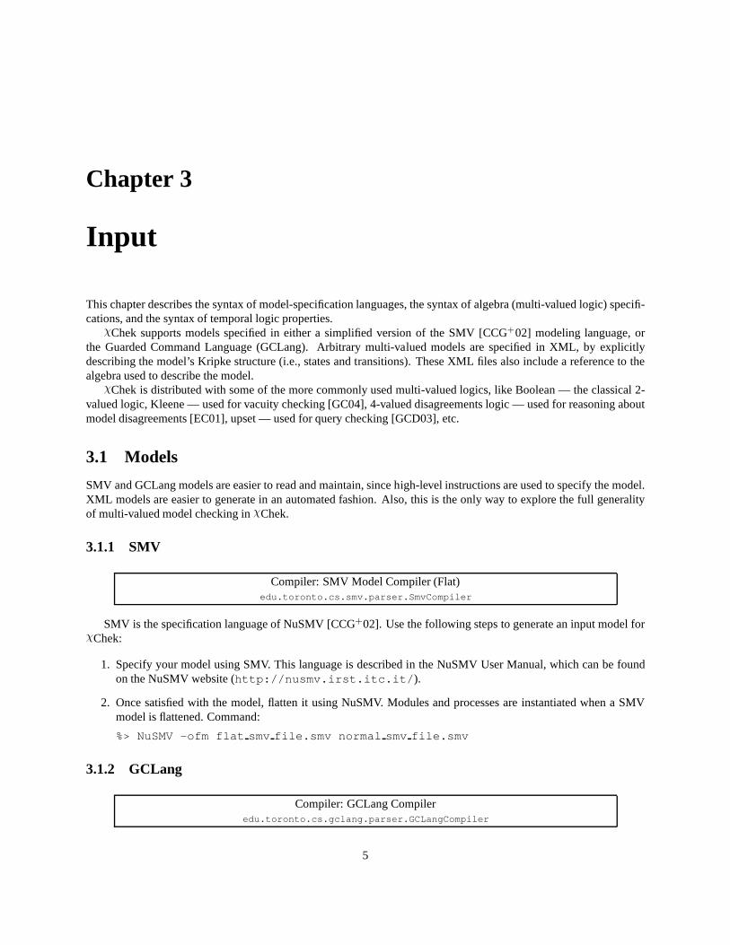
3.1.1 SMV

Compiler: SMV Model Compiler (Flat)edu.toronto.cs.smv.parser.SmvCompiler

SMV is the specification language of NuSMV [CCG+02]. Use the following steps to generate an input model forχChek:

1. Specify your model using SMV. This language is described in the NuSMV User Manual, which can be foundon the NuSMV website (http://nusmv.irst.itc.it/ ).

2. Once satisfied with the model, flatten it using NuSMV. Modules and processes are instantiated when a SMVmodel is flattened. Command:

%> NuSMV -ofm flat smv file.smv normal smv file.smv

3.1.2 GCLang

Compiler: GCLang Compileredu.toronto.cs.gclang.parser.GCLangCompiler

5

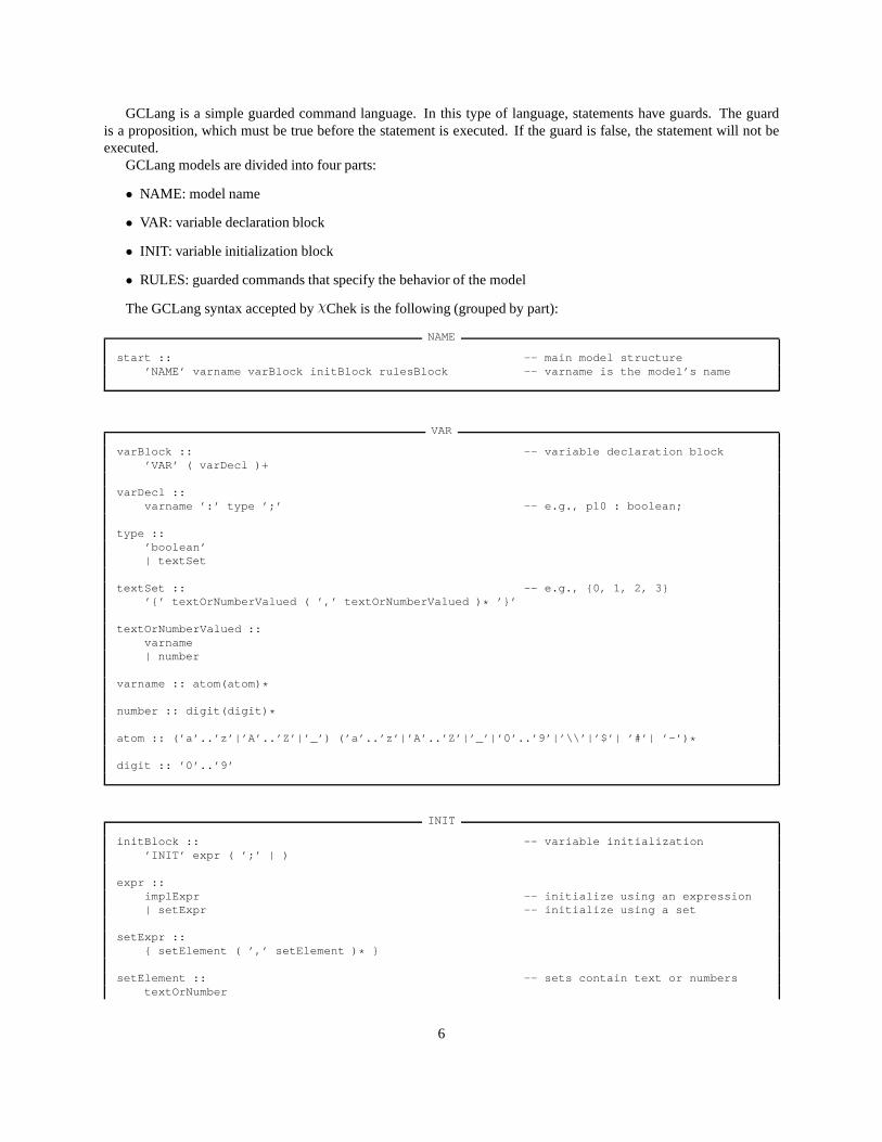
GCLang is a simple guarded command language. In this type of language, statements have guards. The guardis a proposition, which must be true before the statement is executed. If the guard is false, the statement will not beexecuted.

GCLang models are divided into four parts:

• NAME: model name

• VAR: variable declaration block

• INIT: variable initialization block

• RULES: guarded commands that specify the behavior of the model

The GCLang syntax accepted byχChek is the following (grouped by part):

NAME

start :: -- main model structure’NAME’ varname varBlock initBlock rulesBlock -- varname is the model’s name

VAR

varBlock :: -- variable declaration block’VAR’ ( varDecl )+

varDecl ::varname ’:’ type ’;’ -- e.g., p10 : boolean;

type ::’boolean’| textSet

textSet :: -- e.g., {0, 1, 2, 3}’{’ textOrNumberValued ( ’,’ textOrNumberValued ) * ’}’

textOrNumberValued ::varname| number

varname :: atom(atom) *

number :: digit(digit) *

atom :: (’a’..’z’|’A’..’Z’|’_’) (’a’..’z’|’A’..’Z’|’_’ |’0’..’9’|’\\’|’$’| ’#’| ’-’) *

digit :: ’0’..’9’

INIT

initBlock :: -- variable initialization’INIT’ expr ( ’;’ | )

expr ::implExpr -- initialize using an expression| setExpr -- initialize using a set

setExpr ::{ setElement ( ’,’ setElement ) * }

setElement :: -- sets contain text or numberstextOrNumber

6

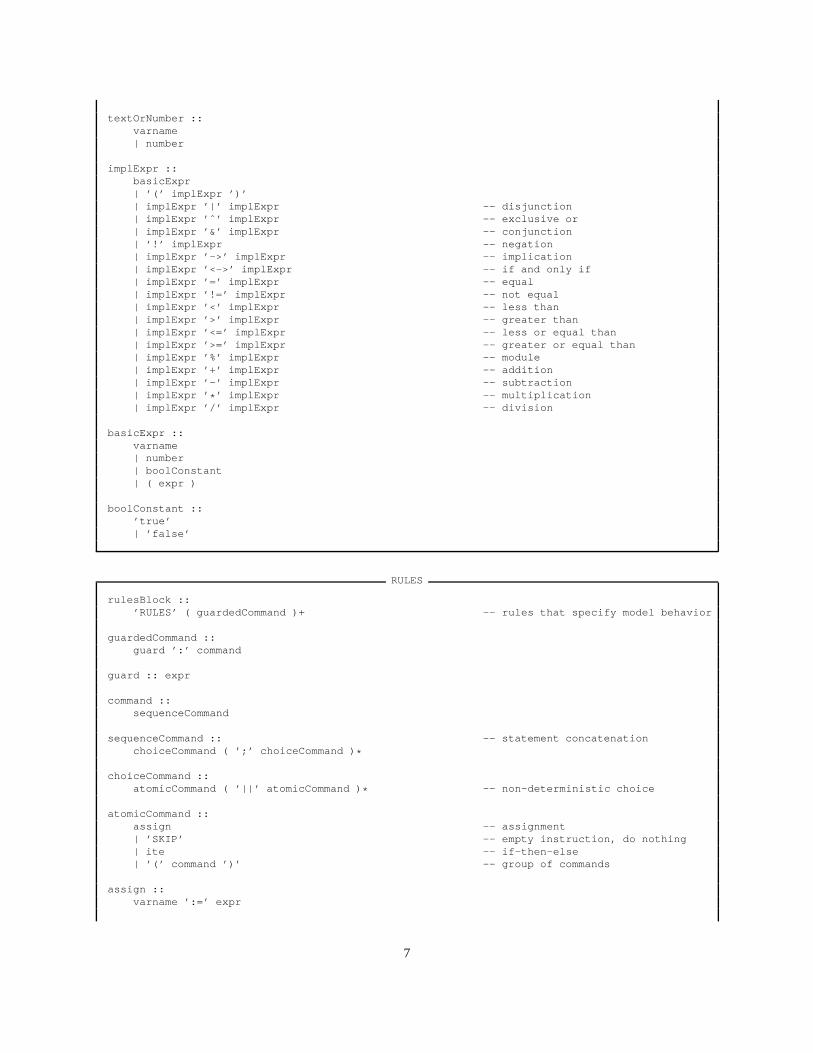
textOrNumber ::varname| number

implExpr ::basicExpr| ’(’ implExpr ’)’| implExpr ’|’ implExpr -- disjunction| implExpr ’ˆ’ implExpr -- exclusive or| implExpr ’&’ implExpr -- conjunction| ’!’ implExpr -- negation| implExpr ’->’ implExpr -- implication| implExpr ’<->’ implExpr -- if and only if| implExpr ’=’ implExpr -- equal| implExpr ’!=’ implExpr -- not equal| implExpr ’<’ implExpr -- less than| implExpr ’>’ implExpr -- greater than| implExpr ’<=’ implExpr -- less or equal than| implExpr ’>=’ implExpr -- greater or equal than| implExpr ’%’ implExpr -- module| implExpr ’+’ implExpr -- addition| implExpr ’-’ implExpr -- subtraction| implExpr ’ * ’ implExpr -- multiplication| implExpr ’/’ implExpr -- division

basicExpr ::varname| number| boolConstant| ( expr )

boolConstant ::’true’| ’false’

RULES

rulesBlock ::’RULES’ ( guardedCommand )+ -- rules that specify model behavior

guardedCommand ::guard ’:’ command

guard :: expr

command ::sequenceCommand

sequenceCommand :: -- statement concatenationchoiceCommand ( ’;’ choiceCommand ) *

choiceCommand ::atomicCommand ( ’||’ atomicCommand ) * -- non-deterministic choice

atomicCommand ::assign -- assignment| ’SKIP’ -- empty instruction, do nothing| ite -- if-then-else| ’(’ command ’)’ -- group of commands

assign ::varname ’:=’ expr

7

ite ::’if (’ expr ’)’ ( ’then’ | ) iteBody -- ’then’ is optional

iteBody ::command ’else’ command ’fi’

Note: Usual precedence rules apply and comments start with “-- ”.

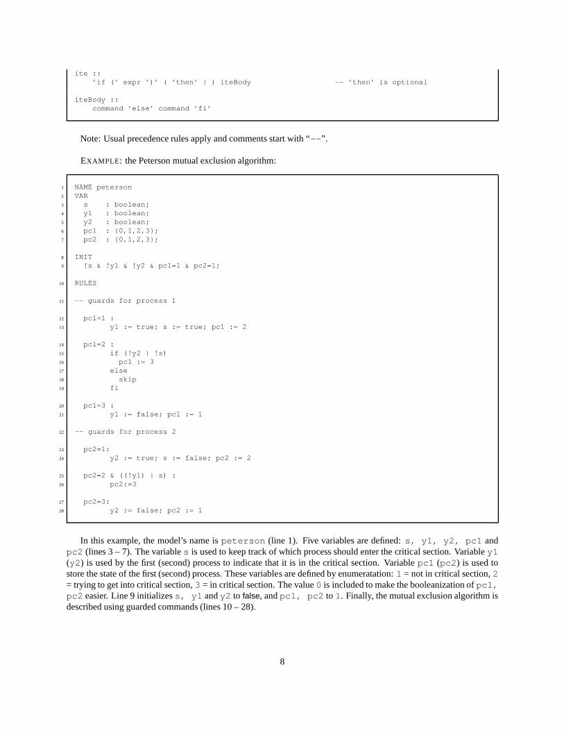
EXAMPLE : the Peterson mutual exclusion algorithm:

1 NAME peterson2 VAR3 s : boolean;4 y1 : boolean;5 y2 : boolean;6 pc1 : {0,1,2,3};7 pc2 : {0,1,2,3};

8 INIT9 !s & !y1 & !y2 & pc1=1 & pc2=1;

10 RULES

11 -- guards for process 1

12 pc1=1 :13 y1 := true; s := true; pc1 := 2

14 pc1=2 :15 if (!y2 | !s)16 pc1 := 317 else18 skip19 fi

20 pc1=3 :21 y1 := false; pc1 := 1

22 -- guards for process 2

23 pc2=1:24 y2 := true; s := false; pc2 := 2

25 pc2=2 & ((!y1) | s) :26 pc2:=3

27 pc2=3:28 y2 := false; pc2 := 1

In this example, the model’s name ispeterson (line 1). Five variables are defined:s, y1, y2, pc1 andpc2 (lines 3 – 7). The variables is used to keep track of which process should enter the critical section. Variabley1(y2 ) is used by the first (second) process to indicate that it is inthe critical section. Variablepc1 (pc2 ) is used tostore the state of the first (second) process. These variables are defined by enumeratation:1 = not in critical section,2= trying to get into critical section,3 = in critical section. The value0 is included to make the booleanization ofpc1,pc2 easier. Line 9 initializess, y1 andy2 to false, andpc1, pc2 to 1. Finally, the mutual exclusion algorithm isdescribed using guarded commands (lines 10 – 28).

8

3.1.3 XML

Compiler: XMLXKripkeModelCompileredu.toronto.cs.xkripke.XMLXKripkeModelCompiler

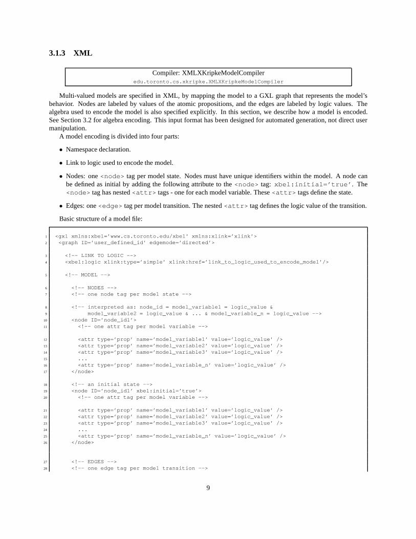
Multi-valued models are specified in XML, by mapping the model to a GXL graph that represents the model’sbehavior. Nodes are labeled by values of the atomic propositions, and the edges are labeled by logic values. Thealgebra used to encode the model is also specified explicitly. In this section, we describe how a model is encoded.See Section 3.2 for algebra encoding. This input format has been designed for automated generation, not direct usermanipulation.

A model encoding is divided into four parts:

• Namespace declaration.

• Link to logic used to encode the model.

• Nodes: one<node> tag per model state. Nodes must have unique identifiers within the model. A node canbe defined as initial by adding the following attribute to the<node> tag: xbel:initial=’true’ . The<node> tag has nested<attr> tags - one for each model variable. These<attr> tags define the state.

• Edges: one<edge> tag per model transition. The nested<attr> tag defines the logic value of the transition.

Basic structure of a model file:

1 <gxl xmlns:xbel=’www.cs.toronto.edu/xbel’ xmlns:xlink =’xlink’>2 <graph ID=’user_defined_id’ edgemode=’directed’>

3 4 <xbel:logic xlink:type=’simple’ xlink:href=’link_to_l ogic_used_to_encode_model’/>

5 

6 7 

8 

10 <node ID=’node_id1’>11 

12 <attr type=’prop’ name=’model_variable1’ value=’logic_ value’ />13 <attr type=’prop’ name=’model_variable2’ value=’logic_ value’ />14 <attr type=’prop’ name=’model_variable3’ value=’logic_ value’ />15 ...16 <attr type=’prop’ name=’model_variable_n’ value=’logic _value’ />17 </node>

18 19 <node ID=’node_id1’ xbel:initial=’true’>20 

21 <attr type=’prop’ name=’model_variable1’ value=’logic_ value’ />22 <attr type=’prop’ name=’model_variable2’ value=’logic_ value’ />23 <attr type=’prop’ name=’model_variable3’ value=’logic_ value’ />24 ...25 <attr type=’prop’ name=’model_variable_n’ value=’logic _value’ />26 </node>

27 28 

9

29 30 <edge from=’node_id1’ to=’node_id2’>31 32 <attr name=’weight’ value=’logic_value’/>33 </edge>

34 </graph>35 </gxl>

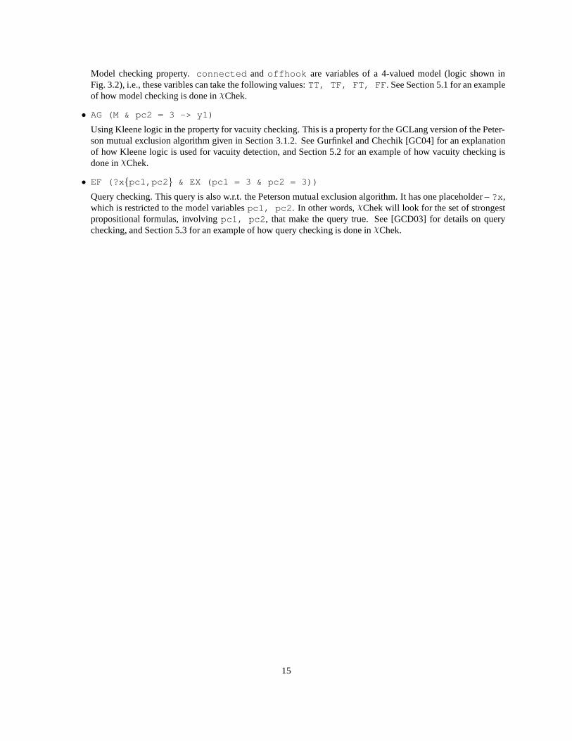
EXAMPLE :

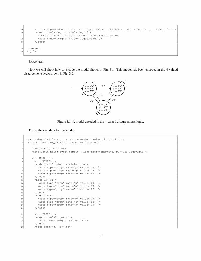
Now we will show how to encode the model shown in Fig. 3.1. Thismodel has been encoded in the 4-valueddisagreements logic shown in Fig. 3.2.

p = TT

q = TF

r = FF

p = FT

q = TT

r = FF

p = TF

q = FT

r = TF

TT

TF

TF

TT

TT

s0s1

s2

Figure 3.1: A model encoded in the 4-valued disagreements logic.

This is the encoding for this model:

1 <gxl xmlns:xbel=’www.cs.toronto.edu/xbel’ xmlns:xlink =’xlink’>2 <graph ID=’model_example’ edgemode=’directed’>

3 4 <xbel:logic xlink:type=’simple’ xlink:href=’examples/ xml/4val-logic.xml’/>

5 6 7 <node ID=’s0’ xbel:initial=’true’>8 <attr type=’prop’ name=’p’ value=’TT’ />9 <attr type=’prop’ name=’q’ value=’TF’ />

10 <attr type=’prop’ name=’r’ value=’FF’ />11 </node>12 <node ID=’s1’>13 <attr type=’prop’ name=’p’ value=’FT’ />14 <attr type=’prop’ name=’q’ value=’TT’ />15 <attr type=’prop’ name=’r’ value=’FF’ />16 </node>17 <node ID=’s2’>18 <attr type=’prop’ name=’p’ value=’TF’ />19 <attr type=’prop’ name=’q’ value=’FT’ />20 <attr type=’prop’ name=’r’ value=’TF’ />21 </node>

22 23 <edge from=’s0’ to=’s1’>24 <attr name=’weight’ value=’TT’/>25 </edge>26 <edge from=’s0’ to=’s2’>

10

27 <attr name=’weight’ value=’TF’/>28 </edge>29 <edge from=’s1’ to=’s1’>30 <attr name=’weight’ value=’TT’/>31 </edge>32 <edge from=’s2’ to=’s0’>33 <attr name=’weight’ value=’TT’/>34 </edge>35 <edge from=’s2’ to=’s1’>36 <attr name=’weight’ value=’TF’/>37 </edge>


An explanation of the various items in the model encoding file:

1-2: GXL namespace declaration, the graph is directed and its id is “modelexample”.

4: location of the logic used to encode the model.

6–21: state definitions. For example, lines 7–11 define states0 . Note that this is an initial state.

22–37: transition definitions. For example, in Fig. 3.1, we see thatthere is aTT transition between statess0 ands1 ,which is encoded in lines 23–25.

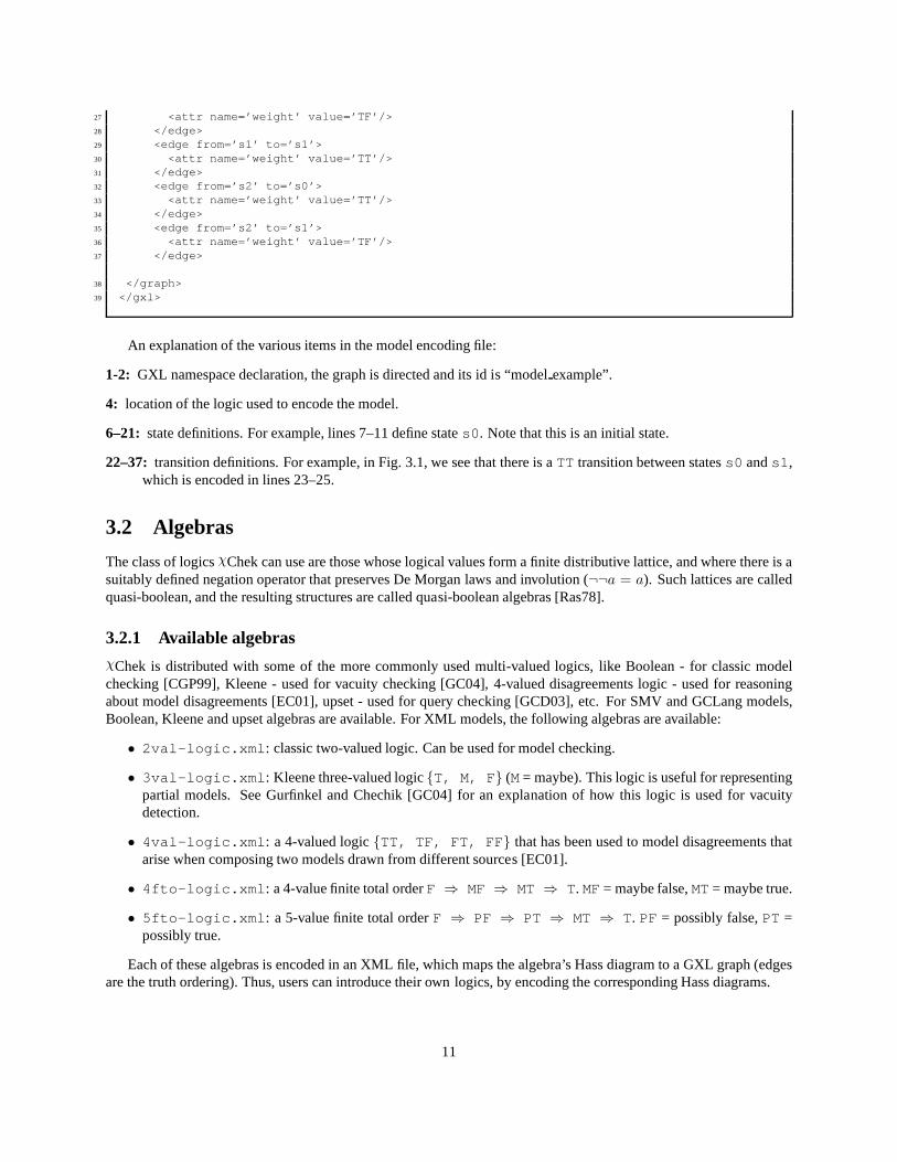
3.2 Algebras

The class of logicsχChek can use are those whose logical values form a finite distributive lattice, and where there is asuitably defined negation operator that preserves De Morganlaws and involution (¬¬a = a). Such lattices are calledquasi-boolean, and the resulting structures are called quasi-boolean algebras [Ras78].

3.2.1 Available algebrasχChek is distributed with some of the more commonly used multi-valued logics, like Boolean - for classic modelchecking [CGP99], Kleene - used for vacuity checking [GC04], 4-valued disagreements logic - used for reasoningabout model disagreements [EC01], upset - used for query checking [GCD03], etc. For SMV and GCLang models,Boolean, Kleene and upset algebras are available. For XML models, the following algebras are available:

• 2val-logic.xml : classic two-valued logic. Can be used for model checking.

• 3val-logic.xml : Kleene three-valued logic{T, M, F } (M= maybe). This logic is useful for representingpartial models. See Gurfinkel and Chechik [GC04] for an explanation of how this logic is used for vacuitydetection.

• 4val-logic.xml : a 4-valued logic{TT, TF, FT, FF } that has been used to model disagreements thatarise when composing two models drawn from different sources [EC01].

• 4fto-logic.xml : a 4-value finite total orderF ⇒ MF ⇒ MT ⇒ T. MF= maybe false,MT= maybe true.

• 5fto-logic.xml : a 5-value finite total orderF ⇒ PF ⇒ PT ⇒ MT ⇒ T. PF = possibly false,PT =possibly true.

Each of these algebras is encoded in an XML file, which maps thealgebra’s Hass diagram to a GXL graph (edgesare the truth ordering). Thus, users can introduce their ownlogics, by encoding the corresponding Hass diagrams.

11

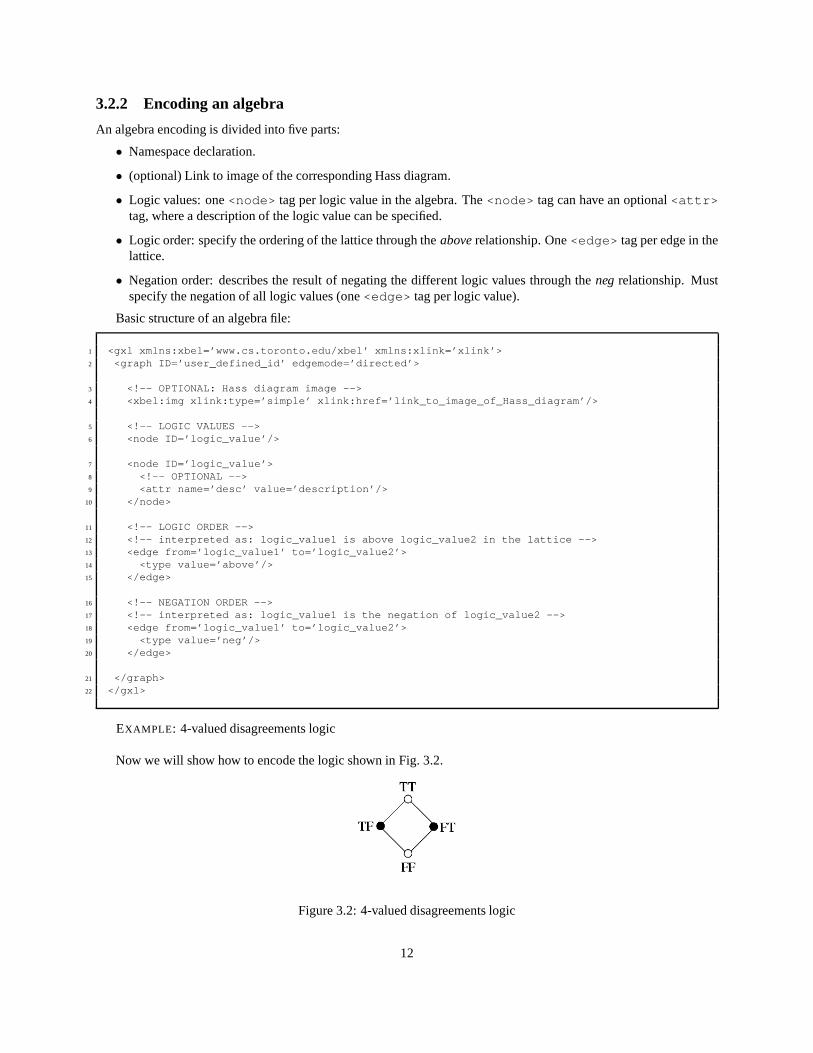
3.2.2 Encoding an algebra

An algebra encoding is divided into five parts:

• Namespace declaration.

• (optional) Link to image of the corresponding Hass diagram.

• Logic values: one<node> tag per logic value in the algebra. The<node> tag can have an optional<attr>tag, where a description of the logic value can be specified.

• Logic order: specify the ordering of the lattice through theaboverelationship. One<edge> tag per edge in thelattice.

• Negation order: describes the result of negating the different logic values through thenegrelationship. Mustspecify the negation of all logic values (one<edge> tag per logic value).

Basic structure of an algebra file:

1 <gxl xmlns:xbel=’www.cs.toronto.edu/xbel’ xmlns:xlink =’xlink’>2 <graph ID=’user_defined_id’ edgemode=’directed’>

3 4 <xbel:img xlink:type=’simple’ xlink:href=’link_to_ima ge_of_Hass_diagram’/>

5 6 <node ID=’logic_value’/>

7 <node ID=’logic_value’>8 9 <attr name=’desc’ value=’description’/>

10 </node>

11 12 13 <edge from=’logic_value1’ to=’logic_value2’>14 <type value=’above’/>15 </edge>

16 17 18 <edge from=’logic_value1’ to=’logic_value2’>19 <type value=’neg’/>20 </edge>


EXAMPLE : 4-valued disagreements logic

Now we will show how to encode the logic shown in Fig. 3.2.

Figure 3.2: 4-valued disagreements logic

12

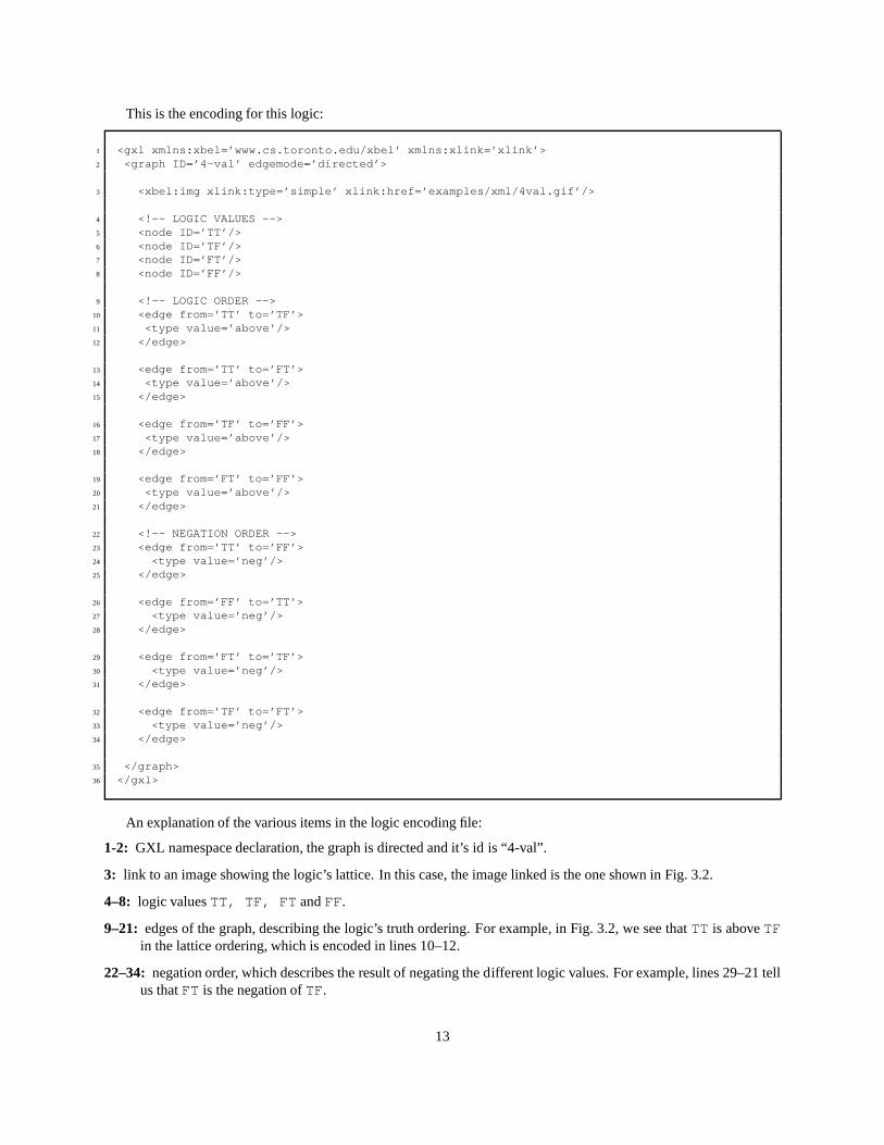
This is the encoding for this logic:

1 <gxl xmlns:xbel=’www.cs.toronto.edu/xbel’ xmlns:xlink =’xlink’>2 <graph ID=’4-val’ edgemode=’directed’>

3 <xbel:img xlink:type=’simple’ xlink:href=’examples/xm l/4val.gif’/>

4 5 <node ID=’TT’/>6 <node ID=’TF’/>7 <node ID=’FT’/>8 <node ID=’FF’/>

9 10 <edge from=’TT’ to=’TF’>11 <type value=’above’/>12 </edge>

13 <edge from=’TT’ to=’FT’>14 <type value=’above’/>15 </edge>

16 <edge from=’TF’ to=’FF’>17 <type value=’above’/>18 </edge>

19 <edge from=’FT’ to=’FF’>20 <type value=’above’/>21 </edge>

22 23 <edge from=’TT’ to=’FF’>24 <type value=’neg’/>25 </edge>

26 <edge from=’FF’ to=’TT’>27 <type value=’neg’/>28 </edge>

29 <edge from=’FT’ to=’TF’>30 <type value=’neg’/>31 </edge>

32 <edge from=’TF’ to=’FT’>33 <type value=’neg’/>34 </edge>


An explanation of the various items in the logic encoding file:

1-2: GXL namespace declaration, the graph is directed and it’s idis “4-val”.

3: link to an image showing the logic’s lattice. In this case, the image linked is the one shown in Fig. 3.2.

4–8: logic valuesTT, TF, FT andFF.

9–21: edges of the graph, describing the logic’s truth ordering. For example, in Fig. 3.2, we see thatTT is aboveTFin the lattice ordering, which is encoded in lines 10–12.

22–34: negation order, which describes the result of negating the different logic values. For example, lines 29–21 tellus thatFT is the negation ofTF.

13

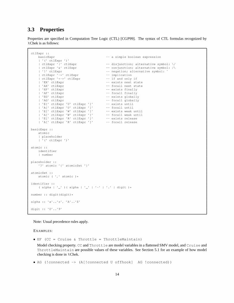
3.3 Properties

Properties are specified in Computation Tree Logic (CTL) [CGP99]. The syntax of CTL formulas recognized byχChek is as follows:

ctlExpr ::basicExpr -- a simple boolean expression| ’(’ ctlExpr ’)’| ctlExpr ’|’ ctlExpr -- disjunction; alternative symbol: \ /| ctlExpr ’&’ ctlExpr -- conjunction; alternative symbol: / \| ’!’ ctlExpr -- negation; alternative symbol: ˜| ctlExpr ’->’ ctlExpr -- implication| ctlExpr ’<->’ ctlExpr -- if and only if| ’EX’ ctlExpr -- exists next state| ’AX’ ctlExpr -- forall next state| ’EF’ ctlExpr -- exists finally| ’AF’ ctlExpr -- forall finally| ’EG’ ctlExpr -- exists globally| ’AG’ ctlExpr -- forall globally| ’E[’ ctlExpr ’U’ ctlExpr ’]’ -- exists until| ’A[’ ctlExpr ’U’ ctlExpr ’]’ -- forall until| ’E[’ ctlExpr ’W’ ctlExpr ’]’ -- exists weak until| ’A[’ ctlExpr ’W’ ctlExpr ’]’ -- forall weak until| ’E[’ ctlExpr ’R’ ctlExpr ’]’ -- exists release| ’A[’ ctlExpr ’R’ ctlExpr ’]’ -- forall release

basicExpr ::atomic| placeholder| ’(’ ctlExpr ’)’

atomic ::identifier| number

placeholder ::’?’ atomic ’{’ atomicSet ’}’

atomicSet ::atomic ( ’,’ atomic ) *

identifier ::( alpha | ’_’ )( alpha | ’_’ | ’-’ | ’.’ | digit ) *

number :: digit(digit) *

alpha :: ’a’..’z’, ’A’..’Z’

digit :: ’0’..’9’

Note: Usual precedence rules apply.

EXAMPLES:

• EF (CC = Cruise & Throttle = ThrottleMaintain)

Model checking property.CCandThrottle are model variables in a flattened SMV model, andCruise andThrottleMaintain are possible values of these variables. See Section 5.1 for an example of how modelchecking is done inχChek.

• AG (!connected -> (A[!connected U offhook] AG !connected))

14

Model checking property.connected and offhook are variables of a 4-valued model (logic shown inFig. 3.2), i.e., these varibles can take the following values: TT, TF, FT, FF . See Section 5.1 for an exampleof how model checking is done inχChek.

• AG (M & pc2 = 3 -> y1)

Using Kleene logic in the property for vacuity checking. This is a property for the GCLang version of the Peter-son mutual exclusion algorithm given in Section 3.1.2. See Gurfinkel and Chechik [GC04] for an explanationof how Kleene logic is used for vacuity detection, and Section 5.2 for an example of how vacuity checking isdone inχChek.

• EF (?x {pc1,pc2 } & EX (pc1 = 3 & pc2 = 3))

Query checking. This query is also w.r.t. the Peterson mutual exclusion algorithm. It has one placeholder –?x ,which is restricted to the model variablespc1, pc2 . In other words,χChek will look for the set of strongestpropositional formulas, involvingpc1, pc2 , that make the querytrue. See [GCD03] for details on querychecking, and Section 5.3 for an example of how query checking is done inχChek.

15

Chapter 4

Guide to the XChek User Interface

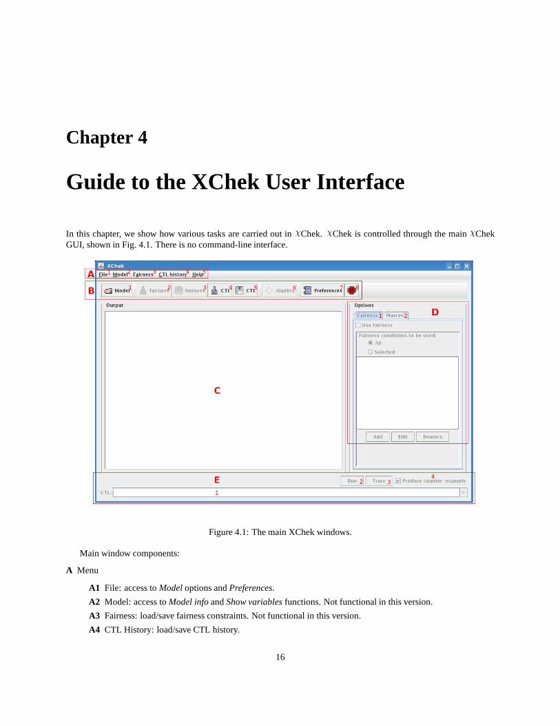
In this chapter, we show how various tasks are carried out inχChek. χChek is controlled through the mainχChekGUI, shown in Fig. 4.1. There is no command-line interface.

Figure 4.1: The main XChek windows.

Main window components:

A Menu

A1 File: access toModeloptions andPreferences.

A2 Model: access toModel infoandShow variablesfunctions. Not functional in this version.

A3 Fairness: load/save fairness constraints. Not functionalin this version.

A4 CTL History: load/save CTL history.

16

A5 Help: access toHelpandAbout.

B Quick access buttons

B1 Model: quick access to theModeloptions.

B2 (load) Fairness: load fairness constraints. Not functional in this version.

B3 (save) Fairness: save fairness constraints. Not functional in this version.

B4 (load) CTL: load CTL history. A CTL history file is just a simple list of properties (one per line).χChekcreates a drop-down menu with these properties, which is accessible from the CTL input box.

B5 (save) CTL: save CTL history.

B6 Algebra: change model algebra. Not functional in this version.

B7 Preferences: quick access toPreferences.

B8 Quit: exitsχChek. If there are properties in the CTL input box,χChek will prompt the user, asking if theseproperties should be saved.

C Main output area: various system messages appear in this area, e.g., success on model loading, results of modelchecking, etc.

D Options: these options are not functional in this version.

D1 Fairness: will allow the specification of fairness constraints, to be applied to the currently loaded model.

D2 Macros: will allow the specification of macros, which can be used to simplify CTL properties and fairnessconstraints.

E CTL area

E1 Input box: properties can be typed directly into this box. Can also be used to access the drop-down menucreated when loading a CTL history file.

E2 Run: runsχChek, checking the property selected in the input box w.r.t.the last model loaded. Results willbe displayed in the main output area (C).

E3 Trace: for simulation purposes. Not functional in this version.

E4 Produce counter-example: when this box is ticked,Runwill also produce a counterexample for the propertybeing checked. The manner in which this counterexample is shown depends on the user’s preferences.

4.1 Loading a model

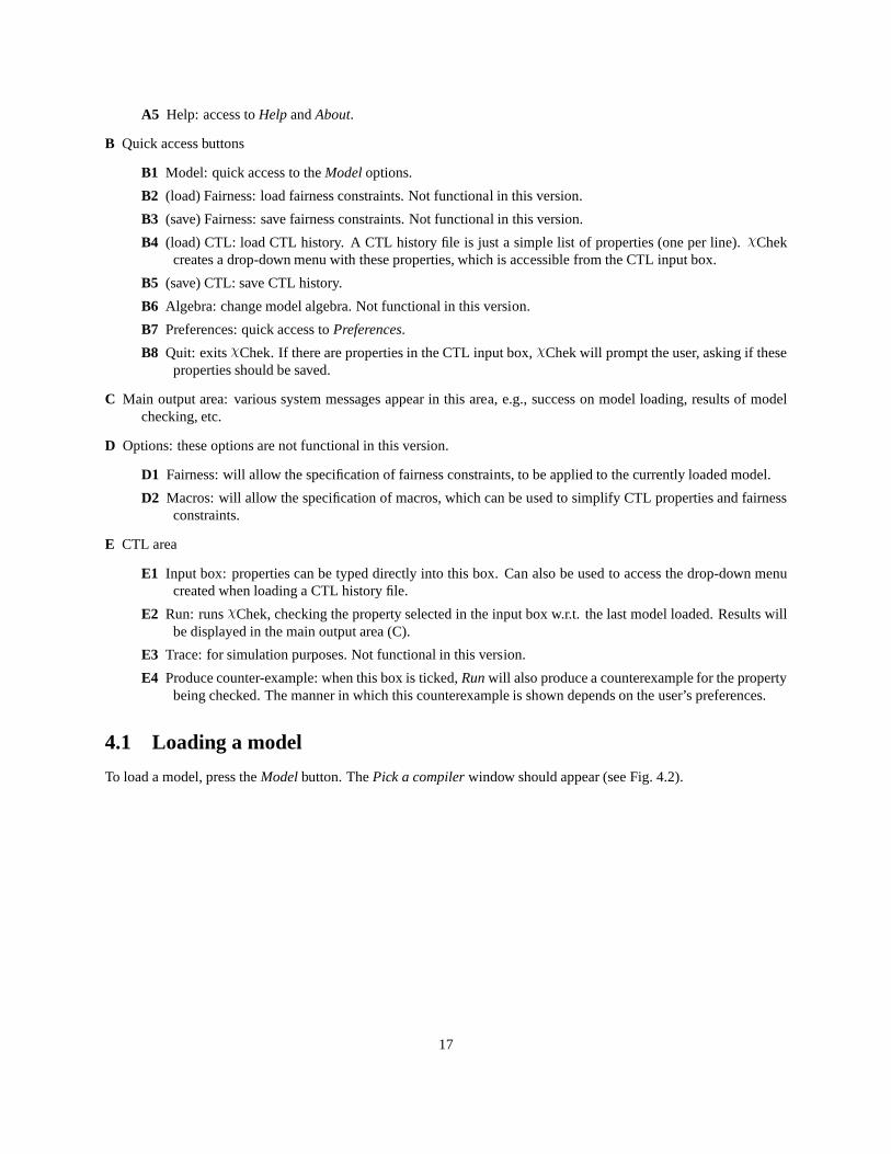
To load a model, press theModelbutton. ThePick a compilerwindow should appear (see Fig. 4.2).

17

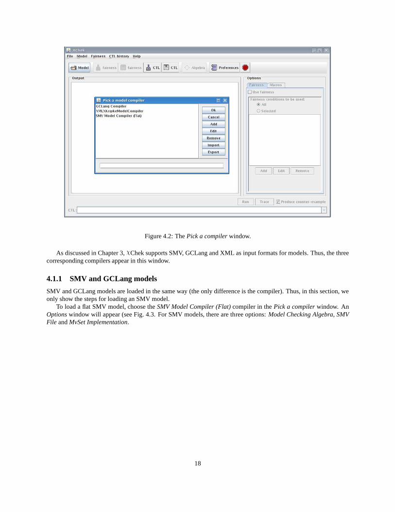
Figure 4.2: ThePick a compilerwindow.

As discussed in Chapter 3,χChek supports SMV, GCLang and XML as input formats for models. Thus, the threecorresponding compilers appear in this window.

4.1.1 SMV and GCLang models

SMV and GCLang models are loaded in the same way (the only difference is the compiler). Thus, in this section, weonly show the steps for loading an SMV model.

To load a flat SMV model, choose theSMV Model Compiler (Flat)compiler in thePick a compilerwindow. AnOptionswindow will appear (see Fig. 4.3. For SMV models, there are three options:Model Checking Algebra, SMVFile andMvSet Implementation.

18

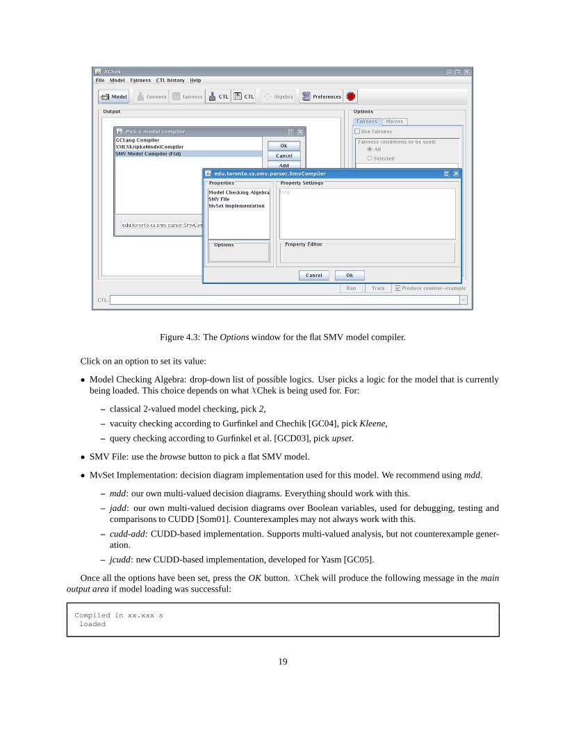
Figure 4.3: TheOptionswindow for the flat SMV model compiler.

Click on an option to set its value:

• Model Checking Algebra: drop-down list of possible logics.User picks a logic for the model that is currentlybeing loaded. This choice depends on whatχChek is being used for. For:

– classical 2-valued model checking, pick2,

– vacuity checking according to Gurfinkel and Chechik [GC04],pick Kleene,

– query checking according to Gurfinkel et al. [GCD03], pickupset.

• SMV File: use thebrowsebutton to pick a flat SMV model.

• MvSet Implementation: decision diagram implementation used for this model. We recommend usingmdd.

– mdd: our own multi-valued decision diagrams. Everything should work with this.

– jadd: our own multi-valued decision diagrams over Boolean variables, used for debugging, testing andcomparisons to CUDD [Som01]. Counterexamples may not always work with this.

– cudd-add: CUDD-based implementation. Supports multi-valued analysis, but not counterexample gener-ation.

– jcudd: new CUDD-based implementation, developed for Yasm [GC05].

Once all the options have been set, press theOK button.χChek will produce the following message in themainoutput areaif model loading was successful:

Compiled in xx.xxx sloaded

19

4.1.2 XML models

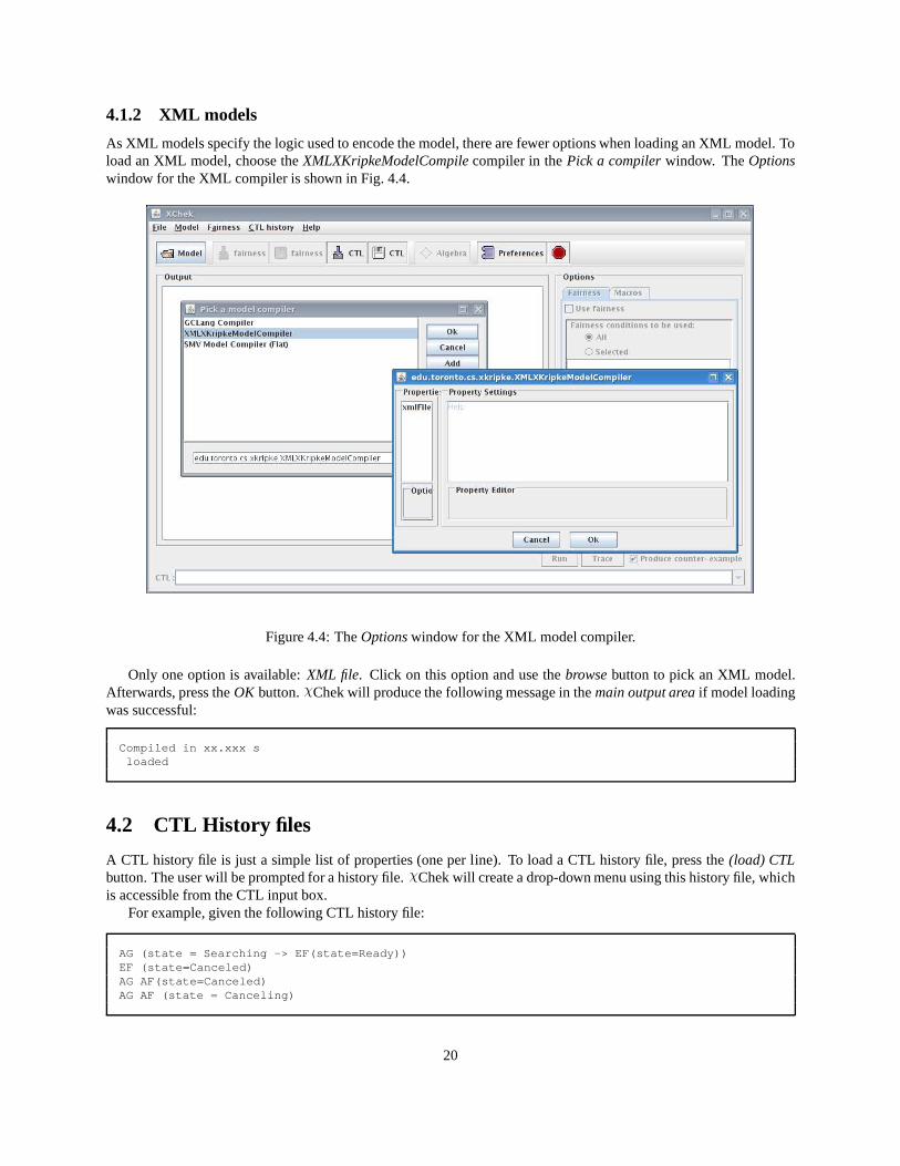
As XML models specify the logic used to encode the model, there are fewer options when loading an XML model. Toload an XML model, choose theXMLXKripkeModelCompilecompiler in thePick a compilerwindow. TheOptionswindow for the XML compiler is shown in Fig. 4.4.

Figure 4.4: TheOptionswindow for the XML model compiler.

Only one option is available:XML file. Click on this option and use thebrowsebutton to pick an XML model.Afterwards, press theOK button.χChek will produce the following message in themain output areaif model loadingwas successful:

Compiled in xx.xxx sloaded

4.2 CTL History files

A CTL history file is just a simple list of properties (one per line). To load a CTL history file, press the(load) CTLbutton. The user will be prompted for a history file.χChek will create a drop-down menu using this history file, whichis accessible from the CTL input box.

For example, given the following CTL history file:

AG (state = Searching -> EF(state=Ready))EF (state=Canceled)AG AF(state=Canceled)AG AF (state = Canceling)

20

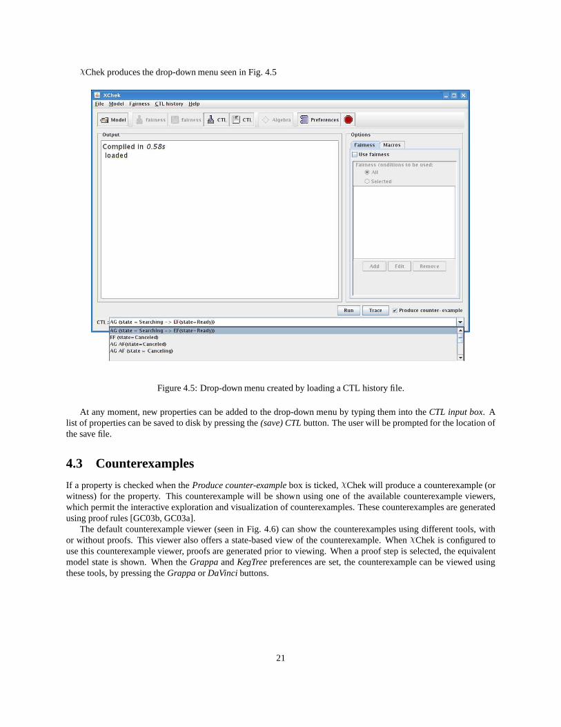
χChek produces the drop-down menu seen in Fig. 4.5

Figure 4.5: Drop-down menu created by loading a CTL history file.

At any moment, new properties can be added to the drop-down menu by typing them into theCTL input box. Alist of properties can be saved to disk by pressing the(save) CTLbutton. The user will be prompted for the location ofthe save file.

4.3 Counterexamples

If a property is checked when theProduce counter-examplebox is ticked,χChek will produce a counterexample (orwitness) for the property. This counterexample will be shown using one of the available counterexample viewers,which permit the interactive exploration and visualization of counterexamples. These counterexamples are generatedusing proof rules [GC03b, GC03a].

The default counterexample viewer (seen in Fig. 4.6) can show the counterexamples using different tools, withor without proofs. This viewer also offers a state-based view of the counterexample. WhenχChek is configured touse this counterexample viewer, proofs are generated priorto viewing. When a proof step is selected, the equivalentmodel state is shown. When theGrappaandKegTreepreferences are set, the counterexample can be viewed usingthese tools, by pressing theGrappaor DaVincibuttons.

21

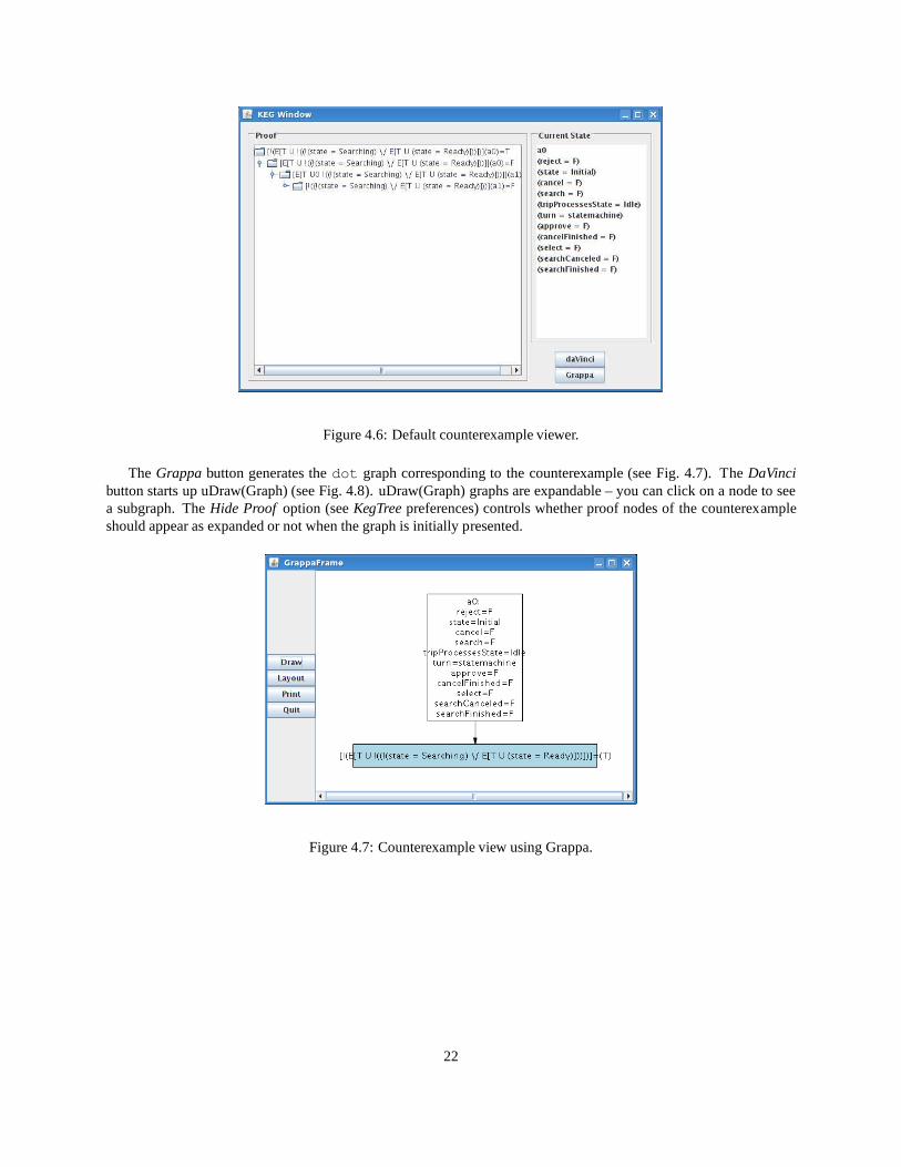
Figure 4.6: Default counterexample viewer.

The Grappabutton generates thedot graph corresponding to the counterexample (see Fig. 4.7). The DaVincibutton starts up uDraw(Graph) (see Fig. 4.8). uDraw(Graph)graphs are expandable – you can click on a node to seea subgraph. TheHide Proof option (seeKegTreepreferences) controls whether proof nodes of the counterexampleshould appear as expanded or not when the graph is initially presented.

Figure 4.7: Counterexample view using Grappa.

22

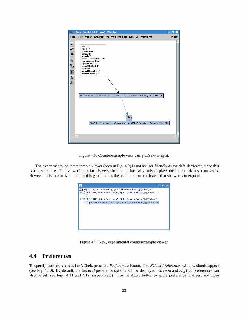
Figure 4.8: Counterexample view using uDraw(Graph).

The experimental counterexample viewer (seen in Fig. 4.9) is not as user-friendly as the default viewer, since thisis a new feature. This viewer’s interface is very simple and basically only displays the internal data strcture as is.However, it is interactive – the proof is generated as the user clicks on the leaves that she wants to expand.

Figure 4.9: New, experimental counterexample viewer.

4.4 Preferences

To specify user preferences forχChek, press thePreferencesbutton. TheXChek Preferenceswindow should appear(see Fig. 4.10). By default, theGeneralpreference options will be displayed.GrappaandKegTreepreferences canalso be set (see Figs. 4.11 and 4.12, respectively). Use theApply button to apply preference changes, and close

23

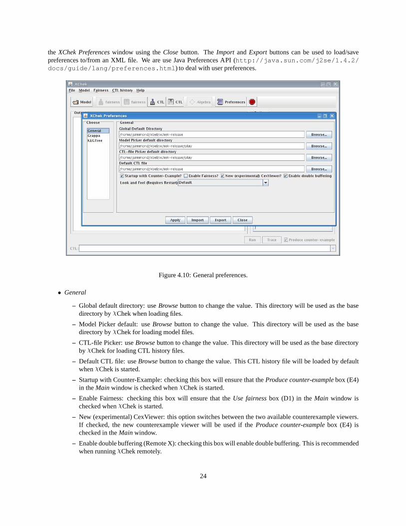
the XChek Preferenceswindow using theClosebutton. TheImport and Export buttons can be used to load/savepreferences to/from an XML file. We are use Java Preferences API (http://java.sun.com/j2se/1.4.2/docs/guide/lang/preferences.html ) to deal with user preferences.

Figure 4.10: General preferences.

• General

– Global default directory: useBrowsebutton to change the value. This directory will be used as thebasedirectory byχChek when loading files.

– Model Picker default: useBrowsebutton to change the value. This directory will be used as thebasedirectory byχChek for loading model files.

– CTL-file Picker: useBrowsebutton to change the value. This directory will be used as thebase directoryby χChek for loading CTL history files.

– Default CTL file: useBrowsebutton to change the value. This CTL history file will be loaded by defaultwhenχChek is started.

– Startup with Counter-Example: checking this box will ensure that theProduce counter-examplebox (E4)in theMain window is checked whenχChek is started.

– Enable Fairness: checking this box will ensure that theUse fairnessbox (D1) in theMain window ischecked whenχChek is started.

– New (experimental) CexViewer: this option switches between the two available counterexample viewers.If checked, the new counterexample viewer will be used if theProduce counter-examplebox (E4) ischecked in theMain window.

– Enable double buffering (Remote X): checking this box will enable double buffering. This is recommendedwhen runningχChek remotely.

24

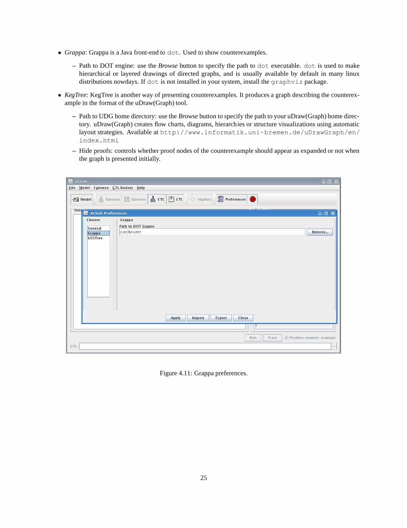
• Grappa: Grappa is a Java front-end todot . Used to show counterexamples.

– Path to DOT engine: use theBrowsebutton to specify the path todot executable.dot is used to makehierarchical or layered drawings of directed graphs, and isusually available by default in many linuxdistributions nowdays. Ifdot is not installed in your system, install thegraphviz package.

• KegTree: KegTree is another way of presenting counterexamples. It produces a graph describing the counterex-ample in the format of the uDraw(Graph) tool.

– Path to UDG home directory: use theBrowsebutton to specify the path to your uDraw(Graph) home direc-tory. uDraw(Graph) creates flow charts, diagrams, hierarchies or structure visualizations using automaticlayout strategies. Available athttp://www.informatik.uni-bremen.de/uDrawGraph/en/index.html

– Hide proofs: controls whether proof nodes of the counterexample should appear as expanded or not whenthe graph is presented initially.

Figure 4.11: Grappa preferences.

25

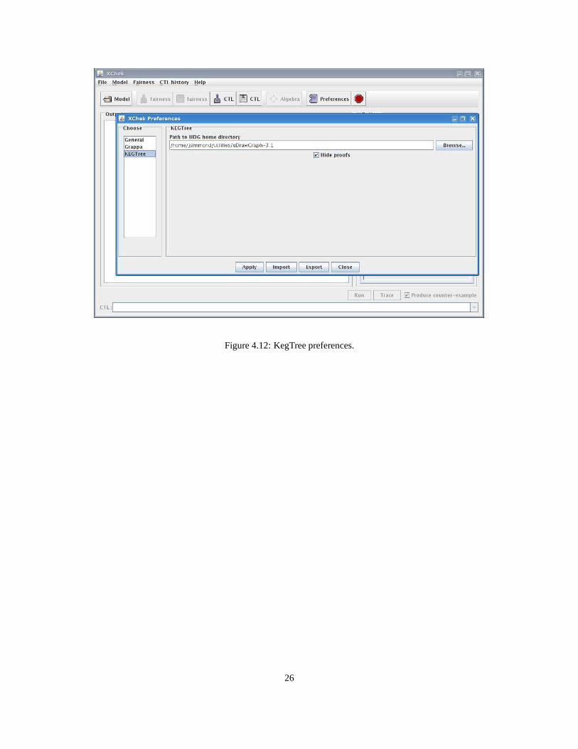
Figure 4.12: KegTree preferences.

26

Chapter 5

Tutorial

In this chapter, we show howχChek can be used for various purposes.

5.1 Model Checking

In the following example, we show howχChek can be used for classical 2-valued model checking.Model: /examples/gclang/trip/trip planning5.gc

1. Main window: press theModelbutton.

2. Pick a compilerwindow: choose theGCLang Compiler.

3. Optionswindow:

• Model Checking Algebra:2

• GCLang file:/examples/gclang/trip/trip planning5.gc

• MvSet Implementation:mdd

4. Optionswindow: pressOK when options have been set. TheMain window should look like the one in Fig. 5.1if the steps uptil now have been followed correctly.

5. CTL input box: type in the following propertyAG (state = Searching -> EF(state=Ready))

6. (Optional) Check theProduce counter-examplebox to produce a counterexample for this property.

7. PressRun. TheMain window should now look like the one in Fig. 5.2. If theProduce counter-examplebox ischecked, the result is shown in a separate window, as described in Section 4.3.

27

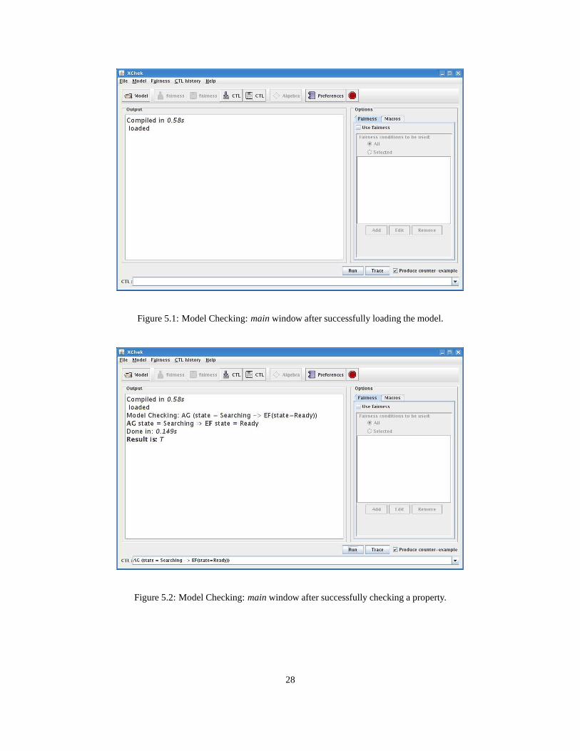
Figure 5.1: Model Checking:mainwindow after successfully loading the model.

Figure 5.2: Model Checking:mainwindow after successfully checking a property.

28

5.2 Vacuity Detection

In the following example, we show howχChek can be used for vacuity detection, according to See Gurfinkel andChechik [GC04]. The 3-valued Kleene logic{F ⇒ M ⇒ T } is used for this purpose. They show that is it possibleto detect the vacuity of a propositional formulaϕ with respect to a formulaψ that is pure inϕ, by (a) replacing alloccurrences ofψ byM , and (b) interpreting the result in the 3-valued Kleene logic. If the new property evaluates toT , thenϕ is vacuouslytrue. If it evaluates toF , thenϕ is vacuouslyfalse. Finally, if ϕ evaluates toM , no decisioncan be made w.r.t. the vacuity of the formula.

Model: /examples/gclang/peterson.gc



3. Optionswindow:

• Model Checking Algebra:Kleene

• GCLang file:/examples/gclang/peterson.gc


4. Optionswindow: pressOK when options have been set.

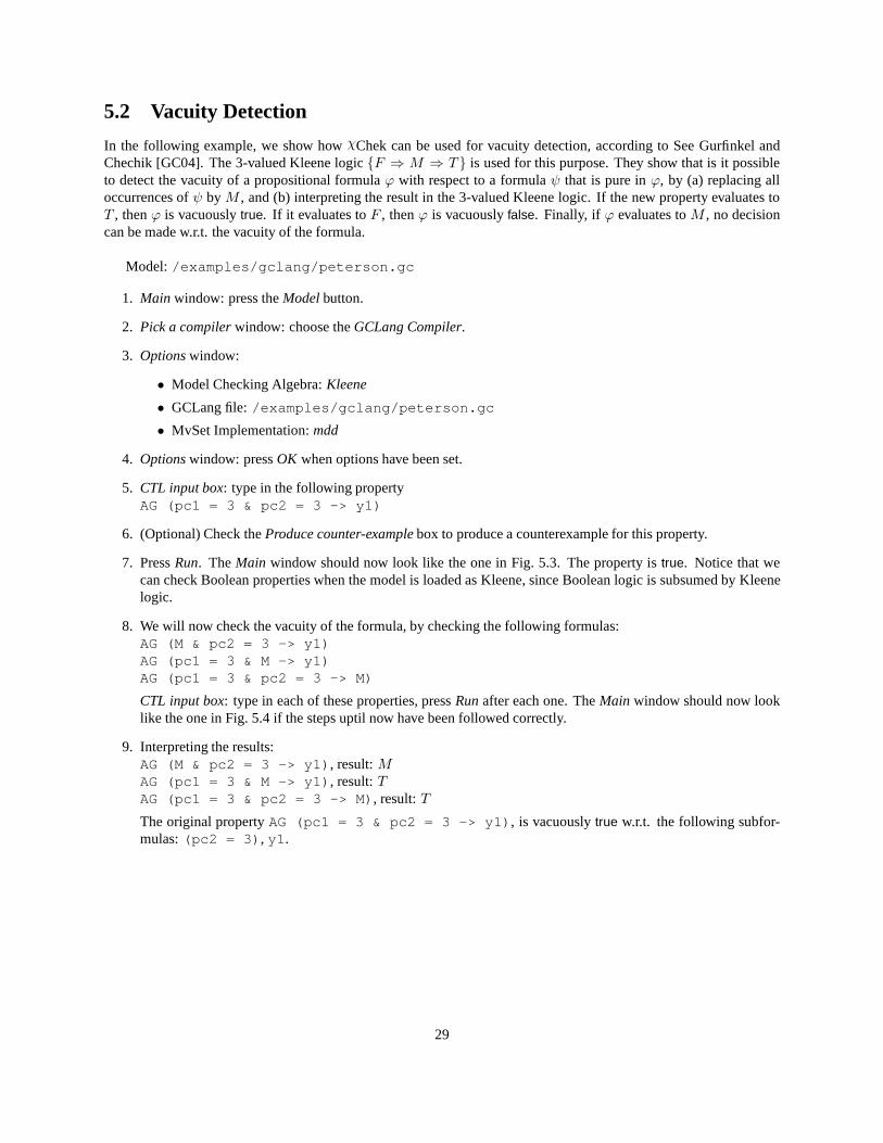
5. CTL input box: type in the following propertyAG (pc1 = 3 & pc2 = 3 -> y1)


7. PressRun. TheMain window should now look like the one in Fig. 5.3. The property is true. Notice that wecan check Boolean properties when the model is loaded as Kleene, since Boolean logic is subsumed by Kleenelogic.

8. We will now check the vacuity of the formula, by checking the following formulas:AG (M & pc2 = 3 -> y1)AG (pc1 = 3 & M -> y1)AG (pc1 = 3 & pc2 = 3 -> M)

CTL input box: type in each of these properties, pressRunafter each one. TheMain window should now looklike the one in Fig. 5.4 if the steps uptil now have been followed correctly.

9. Interpreting the results:AG (M & pc2 = 3 -> y1) , result:MAG (pc1 = 3 & M -> y1) , result:TAG (pc1 = 3 & pc2 = 3 -> M) , result:T

The original propertyAG (pc1 = 3 & pc2 = 3 -> y1) , is vacuouslytrue w.r.t. the following subfor-mulas:(pc2 = 3) , y1 .

29

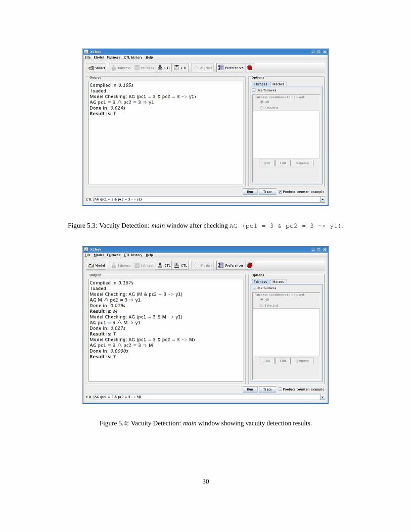
Figure 5.3: Vacuity Detection:mainwindow after checkingAG (pc1 = 3 & pc2 = 3 -> y1) .

Figure 5.4: Vacuity Detection:mainwindow showing vacuity detection results.

30

5.3 Query Checking

In the following example, we show howχChek can be used for query checking (see [GCD03]). Queries are expressedas CTL formulas with missing propositional subformulas, designated by placeholders (“?”). Query Checking finds theformulas that make the querytrue.

Model: /examples/gclang/trip/trip planning5.gc



3. Optionswindow:

• Model Checking Algebra:upset

• GCLang file:/examples/gclang/trip/trip planning5.gc


4. Optionswindow: pressOK when options have been set.

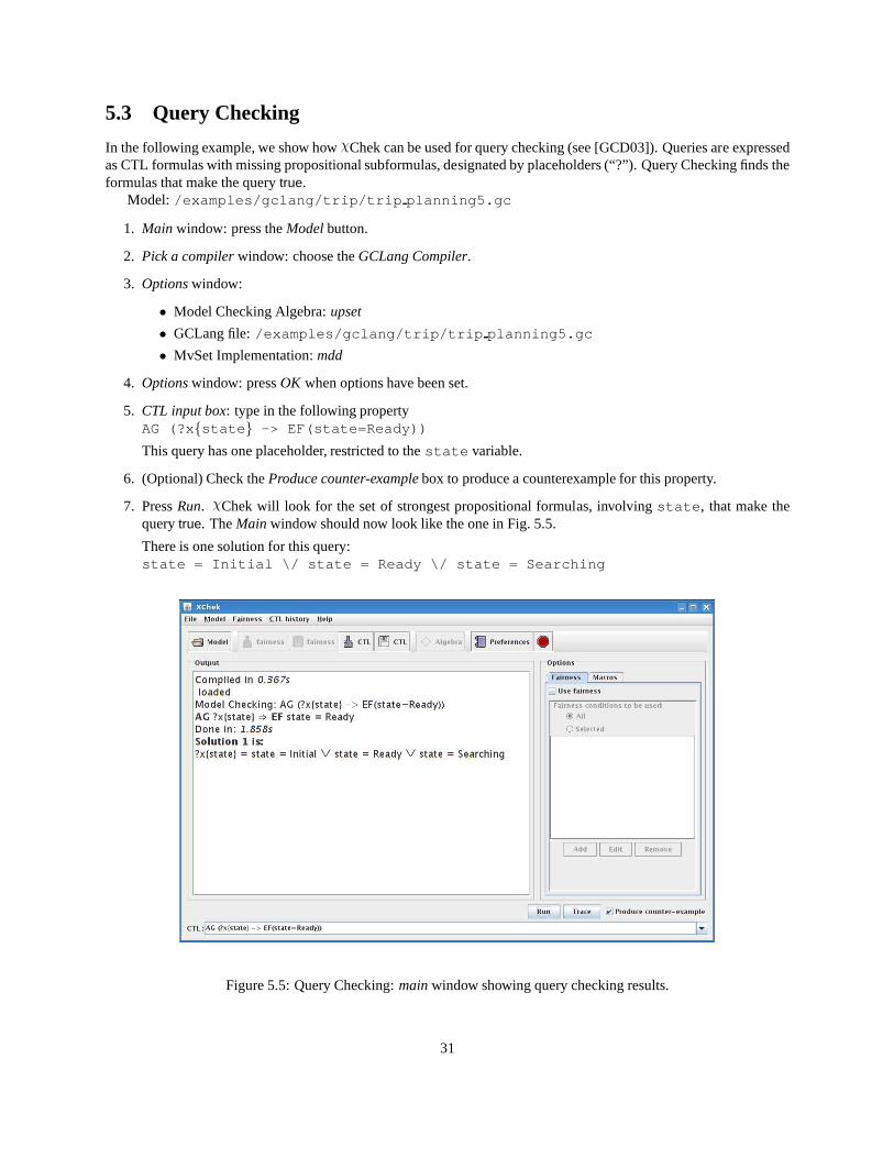
5. CTL input box: type in the following propertyAG (?x {state } -> EF(state=Ready))

This query has one placeholder, restricted to thestate variable.


7. PressRun. χChek will look for the set of strongest propositional formulas, involvingstate , that make thequerytrue. TheMain window should now look like the one in Fig. 5.5.

There is one solution for this query:state = Initial \/ state = Ready \/ state = Searching

Figure 5.5: Query Checking:mainwindow showing query checking results.

31

Bibliography

[CCG+02] A. Cimatti, E. M. Clarke, E. Giunchiglia, F. Giunchiglia, M. Pistore, M. Roveri, R. Sebastiani, and A. Tac-chella. NUSMV 2: An OpenSource Tool for Symbolic Model Checking. InProceedings of CAV’02,volume 2404 ofLNCS, pages 359–364, 2002.

[CDEG03] M. Chechik, B. Devereux, S. Easterbrook, and A. Gurfinkel. Multi-Valued Symbolic Model-Checking.ACM Transactions on Software Engineering and Methodology, 12(4):1–38, October 2003.

[CDG02] M. Chechik, B. Devereux, and A. Gurfinkel.χChek: A Multi-Valued Model-Checker. InProceedings of14th International Conference on Computer-Aided Verification (CAV’02), volume 2404 ofLNCS, pages505–509, Copenhagen, Denmark, July 2002. Springer.

[CGD+06] M. Chechik, A. Gurfinkel, B. Devereux, A. Lai, and S. Easterbrook. “Symbolic Data Structures forMulti-Valued Model-Checking”.Formal Methods in System Design, 29(3), 2006.

[CGP99] E. Clarke, O. Grumberg, and D. Peled.Model Checking. MIT Press, 1999.

[EC01] S. Easterbrook and M. Chechik. “A Framework for Multi-Valued Reasoning over Inconsistent View-points”. InProceedings of International Conference on Software Engineering (ICSE’01), pages 411–420,Toronto, Canada, May 2001. IEEE Computer Society Press.

[GC03a] A. Gurfinkel and M. Chechik. Generating Counterexamples for Multi-Valued Model-Checking. InProceedings of Formal Methods Europe (FME’03), volume 2805 ofLNCS, pages 503–521, Pisa, Italy,September 2003. Springer.

[GC03b] A. Gurfinkel and M. Chechik. Proof-like Counterexamples. InProceedings of 9th International Confer-ence on Tools and Algorithms for the Construction and Analysis of Systems (TACAS’03), volume 2619 ofLNCS, pages 160–175, Warsaw, Poland, April 2003. Springer.

[GC04] A. Gurfinkel and M. Chechik. How Vacuous Is Vacuous? InProceedings of TACAS’04, volume 2988 ofLNCS, pages 451–466, March 2004.

[GC05] A. Gurfinkel and M. Chechik. YASM: Model-Checking Software with Belnap Logic. Technical Report533, University of Toronto, April 2005.

[GCD03] A. Gurfinkel, M. Chechik, and B. Devereux. Temporal Logic Query Checking: A Tool for Model Explo-ration. IEEE Transactions on Software Engineering, 29(10):898–914, October 2003.

[Gur02] A. Gurfinkel. Multi-Valued Symbolic Model-Checking: Fairness, Counter-Examples, Running Time.Master’s thesis, University of Toronto, Department of Computer Science, October 2002.

[Ras78] H. Rasiowa.An Algebraic Approach to Non-Classical Logics. Studies in Logic and the Foundations ofMathematics. Amsterdam: North-Holland, 1978.

[Som01] F. Somenzi. “CUDD: CU Decision Diagram Package Release”, 2001.

32

χChek RC2 User Manual - University of Torontoarie/xchek/xchek_user_manual.pdf · 4.1 Loading a...

Documents

Transcript of χChek RC2 User Manual - University of Torontoarie/xchek/xchek_user_manual.pdf · 4.1 Loading a...