Checking univariate normality Normal probability plots Histograms Bivariate normal density with =0, =0, σ = 1, σ =1 ρ=0.9 1µ 2µ 1 2

(in Maple) > plot3d(exp(-(x^2-2*0.9*x*y+y^2)/(2*(1-0.9^2)))/(2*Pi*sqrt(1-0.9^2)),x=-4..4,y=-4..4);

>

1

Bivariate normal density with =0, =0, σ = 1, σ =2 ρ=0.9 1µ 2µ 1 2

(in Maple) > plot3d(exp(-(x1^2-2*0.9*x1*(x2/2)+(x2/2)^2)/(2*(1-0.9^2)))/(2*2*Pi*sqrt(1-0.9^2)),x1=-4..4,x2=-4..4);

>

2

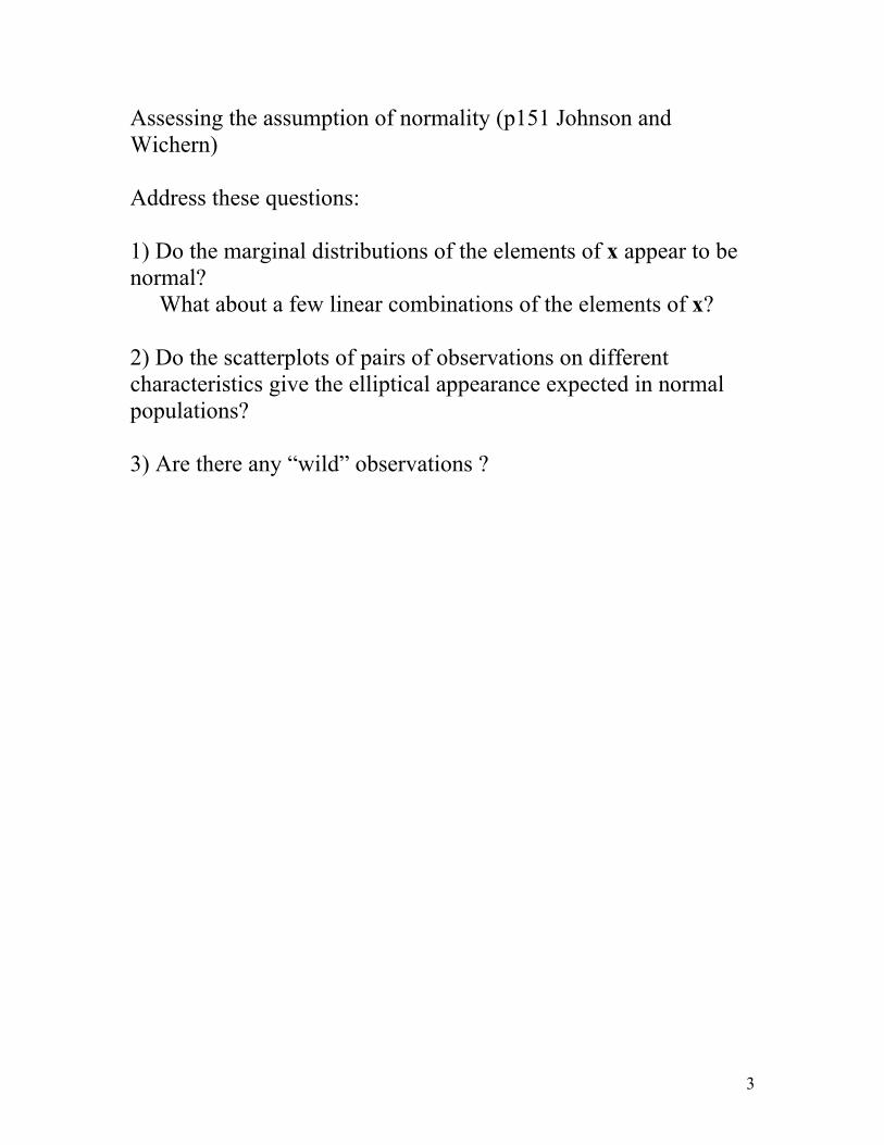
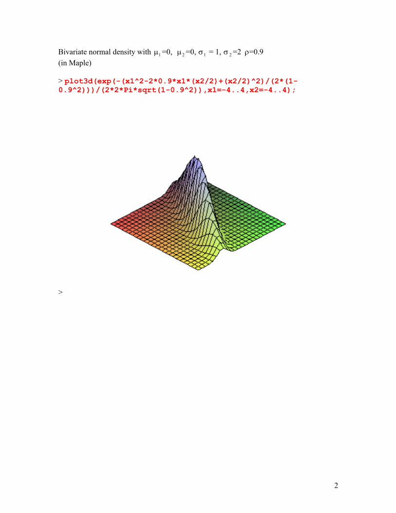
Assessing the assumption of normality (p151 Johnson and Wichern) Address these questions: 1) Do the marginal distributions of the elements of x appear to be normal? What about a few linear combinations of the elements of x? 2) Do the scatterplots of pairs of observations on different characteristics give the elliptical appearance expected in normal populations? 3) Are there any “wild” observations ?

3

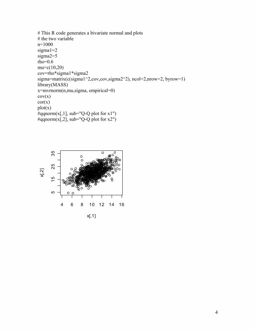
# This R code generates a bivariate normal and plots # the two variable n=1000 sigma1=2 sigma2=5 rho=0.6 mu=c(10,20) cov=rho*sigma1*sigma2 sigma=matrix(c(sigma1^2,cov,cov,sigma2^2), ncol=2,nrow=2, byrow=1) library(MASS) x=mvrnorm(n,mu,sigma, empirical=0) cov(x) cor(x) plot(x) #qqnorm(x[,1], sub="Q-Q plot for x1") #qqnorm(x[,2], sub="Q-Q plot for x2")

4 6 8 10 12 14 16

515

2535

x[,1]

x[,2

]

4

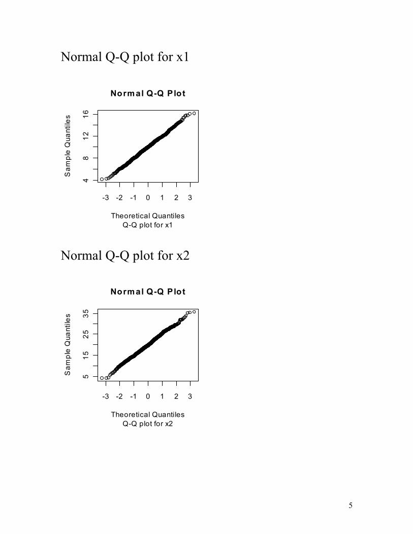
Normal Q-Q plot for x1

-3 -2 -1 0 1 2 3

48

1216

Normal Q-Q Plot

Q-Q plot for x1Theoretical Quantiles

Sam

ple

Qua

ntile

s

Normal Q-Q plot for x2

-3 -2 -1 0 1 2 3

515

2535

Normal Q-Q Plot

Q-Q plot for x2Theoretical Quantiles

Sam

ple

Qua

ntile

s

5

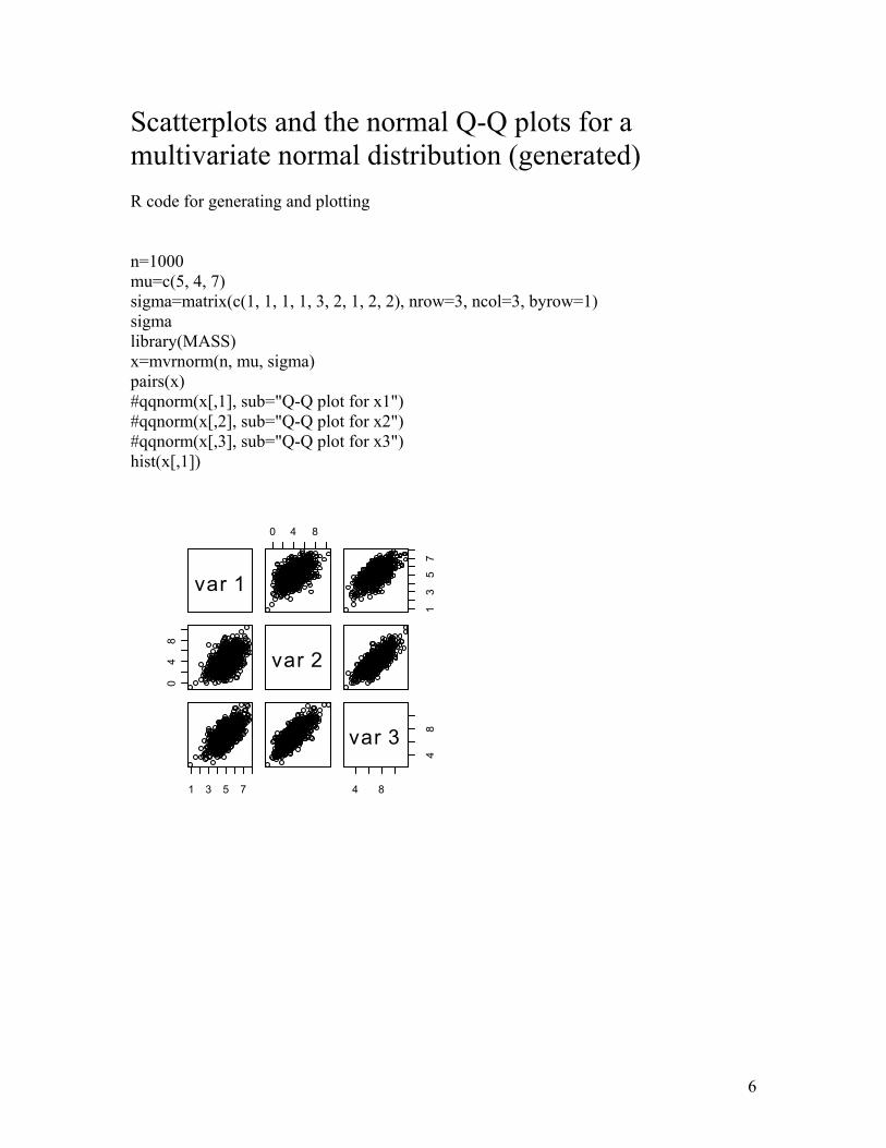
Scatterplots and the normal Q-Q plots for a multivariate normal distribution (generated) R code for generating and plotting n=1000 mu=c(5, 4, 7) sigma=matrix(c(1, 1, 1, 1, 3, 2, 1, 2, 2), nrow=3, ncol=3, byrow=1) sigma library(MASS) x=mvrnorm(n, mu, sigma) pairs(x) #qqnorm(x[,1], sub="Q-Q plot for x1") #qqnorm(x[,2], sub="Q-Q plot for x2") #qqnorm(x[,3], sub="Q-Q plot for x3") hist(x[,1])

var 1

0 4 8

13

57

04

8

var 2

1 3 5 7 4 8

48var 3

6

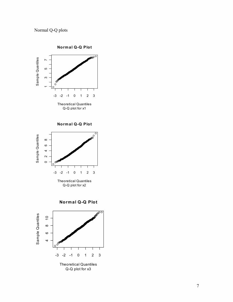
Normal Q-Q plots

-3 -2 -1 0 1 2 3

13

57

Normal Q-Q Plot

Q-Q plot for x1Theoretical Quantiles

Sam

ple

Qua

ntile

s

-3 -2 -1 0 1 2 3

02

46

8

Normal Q-Q Plot

Q-Q plot for x2Theoretical Quantiles

Sam

ple

Qua

ntile

s

-3 -2 -1 0 1 2 3

46

810

Normal Q-Q Plot

Q-Q plot for x3Theoretical Quantiles

Sam

ple

Qua

ntile

s

7

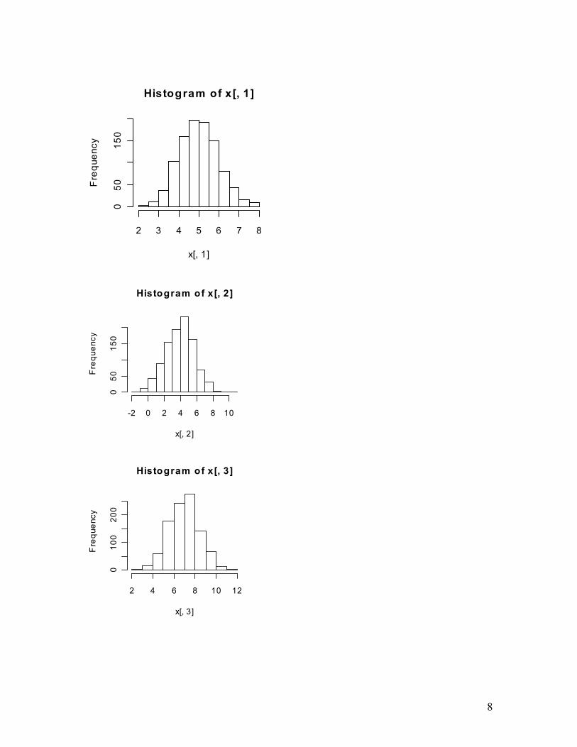
Histogram of x[, 1]

x[, 1]

Fre

quen

cy

2 3 4 5 6 7 8

050

150

Histogram of x[, 2]

x[, 2]

Fre

quen

cy

-2 0 2 4 6 8 10

050

150

Histogram of x[, 3]

x[, 3]

Fre

quen

cy

2 4 6 8 10 12

010

020

0

8

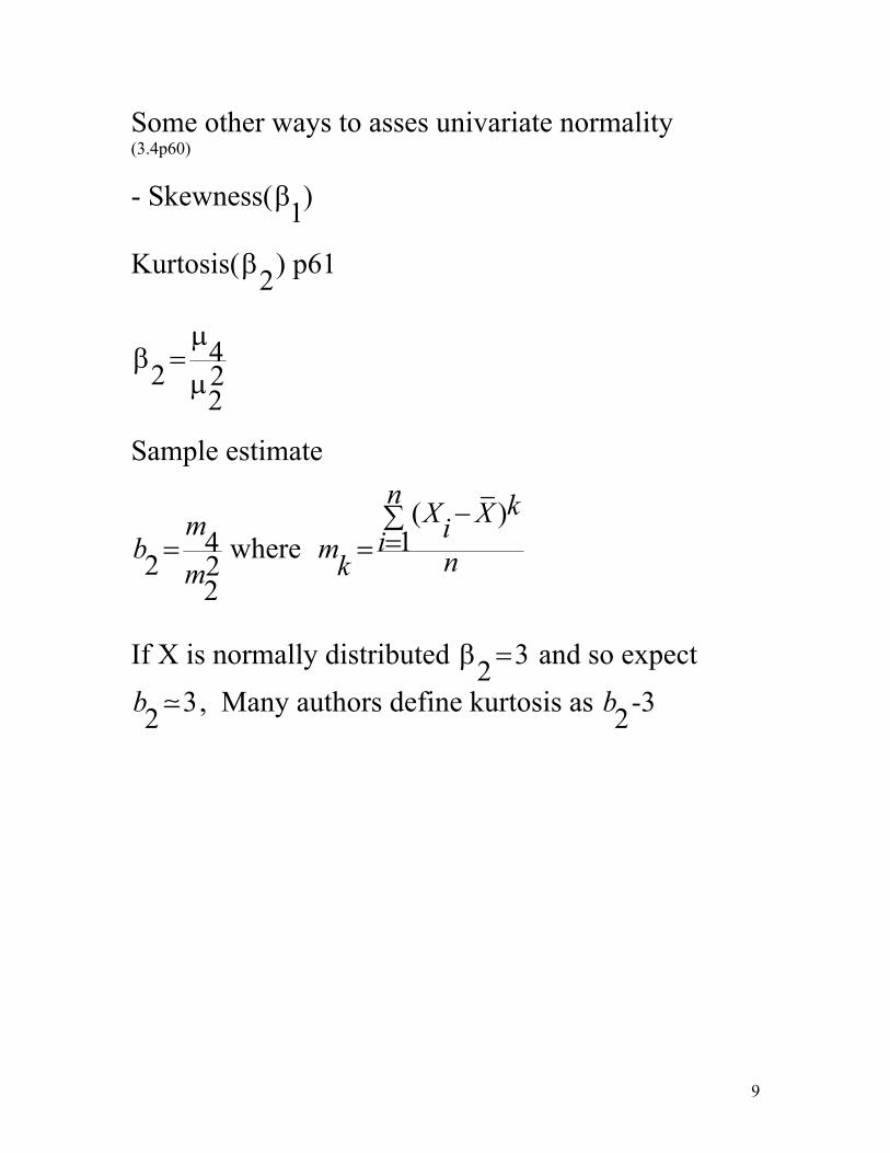
Some other ways to asses univariate normality (3.4p60)

- Skewness( ) 1β

Kurtosis( ) p61 2β

42 2

2

µβ

µ=

Sample estimate

42 2m

bm

=2

where ( )

1

n kX Xiim nk

−∑==

If X is normally distributed and so expect

, Many authors define kurtosis as b -3 32β =

32b 2

9

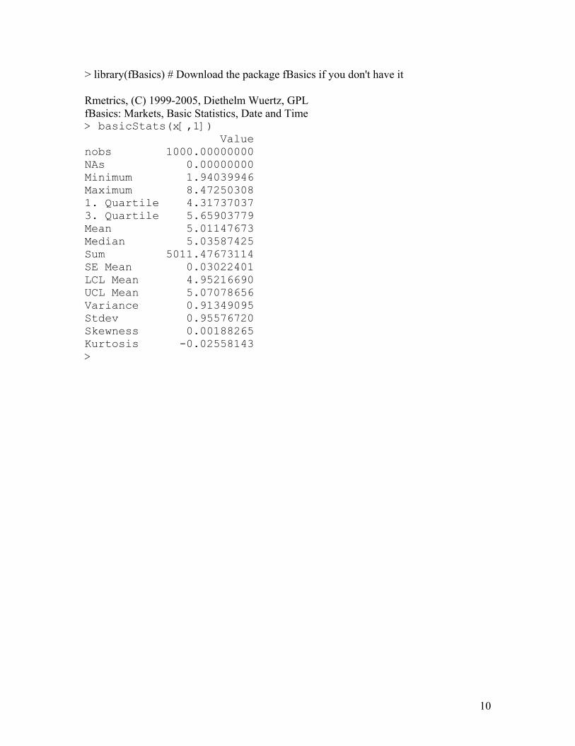
> library(fBasics) # Download the package fBasics if you don't have it Rmetrics, (C) 1999-2005, Diethelm Wuertz, GPL fBasics: Markets, Basic Statistics, Date and Time > basicStats(x[,1]) Value nobs 1000.00000000 NAs 0.00000000 Minimum 1.94039946 Maximum 8.47250308 1. Quartile 4.31737037 3. Quartile 5.65903779 Mean 5.01147673 Median 5.03587425 Sum 5011.47673114 SE Mean 0.03022401 LCL Mean 4.95216690 UCL Mean 5.07078656 Variance 0.91349095 Stdev 0.95576720 Skewness 0.00188265 Kurtosis -0.02558143 >

10

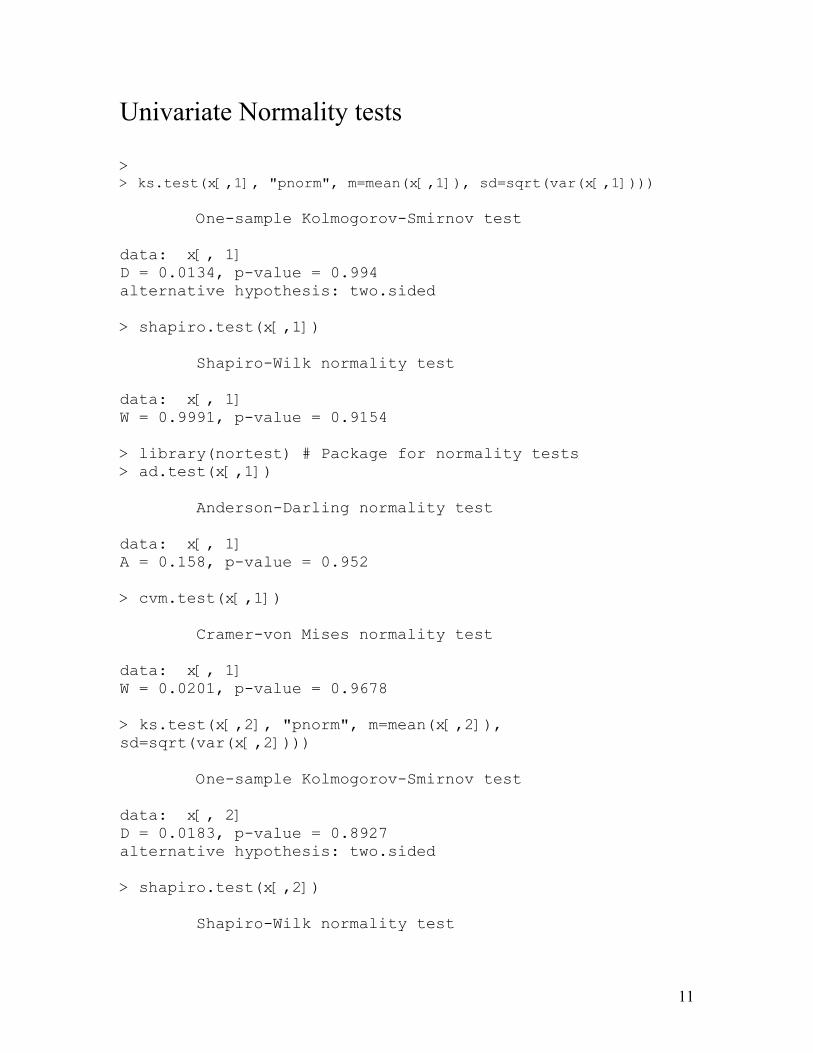
Univariate Normality tests > > ks.test(x[,1], "pnorm", m=mean(x[,1]), sd=sqrt(var(x[,1]))) One-sample Kolmogorov-Smirnov test data: x[, 1] D = 0.0134, p-value = 0.994 alternative hypothesis: two.sided > shapiro.test(x[,1]) Shapiro-Wilk normality test data: x[, 1] W = 0.9991, p-value = 0.9154 > library(nortest) # Package for normality tests > ad.test(x[,1]) Anderson-Darling normality test data: x[, 1] A = 0.158, p-value = 0.952 > cvm.test(x[,1]) Cramer-von Mises normality test data: x[, 1] W = 0.0201, p-value = 0.9678 > ks.test(x[,2], "pnorm", m=mean(x[,2]), sd=sqrt(var(x[,2]))) One-sample Kolmogorov-Smirnov test data: x[, 2] D = 0.0183, p-value = 0.8927 alternative hypothesis: two.sided > shapiro.test(x[,2]) Shapiro-Wilk normality test

11

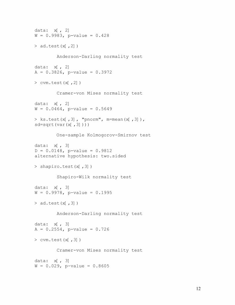
data: x[, 2] W = 0.9983, p-value = 0.428 > ad.test(x[,2]) Anderson-Darling normality test data: x[, 2] A = 0.3826, p-value = 0.3972 > cvm.test(x[,2]) Cramer-von Mises normality test data: x[, 2] W = 0.0464, p-value = 0.5649 > ks.test(x[,3], "pnorm", m=mean(x[,3]), sd=sqrt(var(x[,3]))) One-sample Kolmogorov-Smirnov test data: x[, 3] D = 0.0148, p-value = 0.9812 alternative hypothesis: two.sided > shapiro.test(x[,3]) Shapiro-Wilk normality test data: x[, 3] W = 0.9978, p-value = 0.1995 > ad.test(x[,3]) Anderson-Darling normality test data: x[, 3] A = 0.2554, p-value = 0.726 > cvm.test(x[,3]) Cramer-von Mises normality test data: x[, 3] W = 0.029, p-value = 0.8605

12

13

>