CHE3162 Lecture 9

PID Controllers - Calculating &

Eliminating Offset

Chapter 7&8: Marlin Chapter 6: Smith & Corripio

Learning objectives

• Understand P control and calculate offset for setpoint and disturbance changes

• Understand how PI control eliminates offset • Understand how tuning control loop parameters

K, TI and τd affect response of control loops • Be able to prove the magnitude or absence of

offset using TF and final value theorem

PID response matches “common sense”

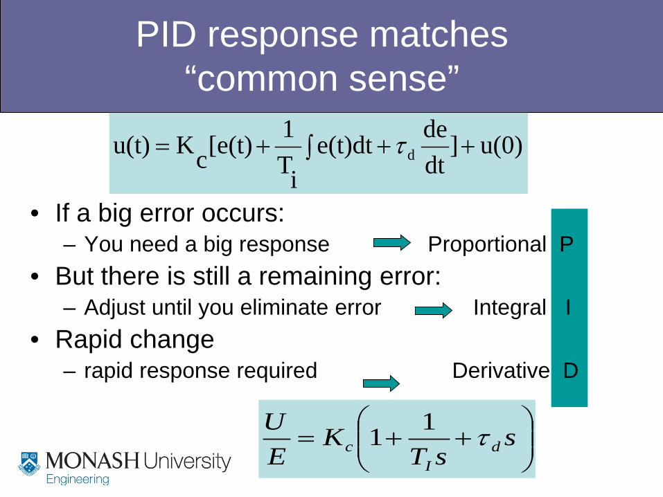
• If a big error occurs: – You need a big response Proportional P

• But there is still a remaining error: – Adjust until you eliminate error Integral I

• Rapid change – rapid response required Derivative D

∫ +++= u(0)]dtdee(t)dt

iT1[e(t)cKu(t) dτ

++= s

sTK

EU

dI

c τ11

General Block Diagram

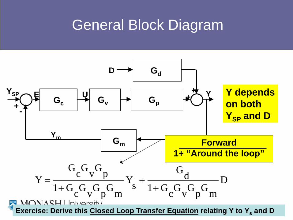
Y Gc

U

Gm Ym

Gd D

+ + YSP E

+ - Gv Gp

DmGpGvGcG1

dGsY

mGpGvGcG1pGvGcG

Y+

++

=

Y depends on both YSP and D

Exercise: Derive this Closed Loop Transfer Equation relating Y to Ys and D

Forward 1+ “Around the loop”

P control

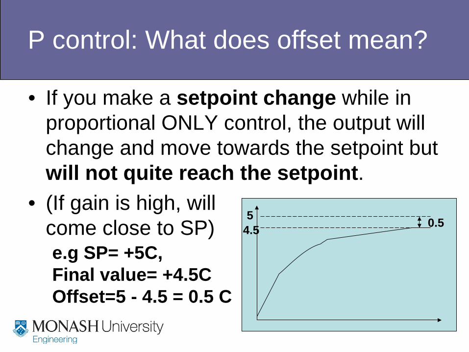
P control: What does offset mean?

• If you make a setpoint change while in proportional ONLY control, the output will change and move towards the setpoint but will not quite reach the setpoint.

• (If gain is high, will come close to SP)

5 0.5 4.5

e.g SP= +5C, Final value= +4.5C Offset=5 - 4.5 = 0.5 C

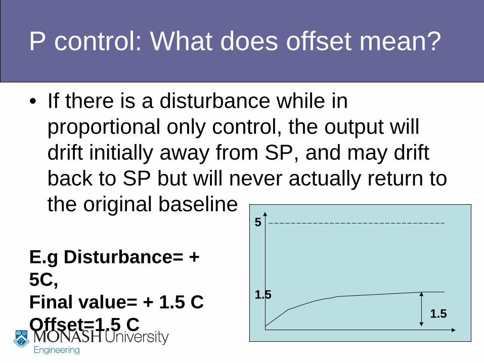
P control: What does offset mean?

• If there is a disturbance while in proportional only control, the output will drift initially away from SP, and may drift back to SP but will never actually return to the original baseline

5

1.5 1.5

E.g Disturbance= + 5C, Final value= + 1.5 C Offset=1.5 C

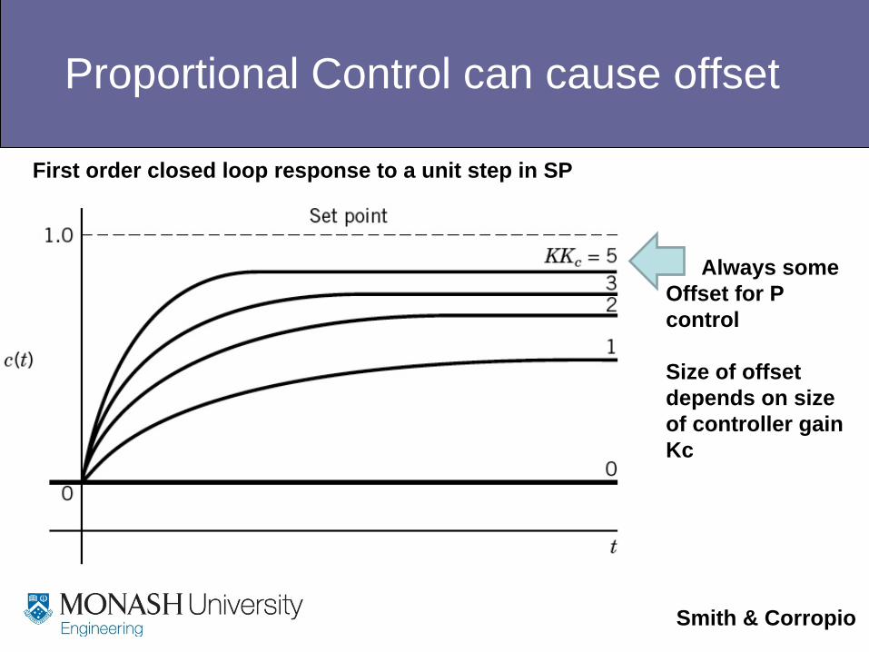
Proportional Control can cause offset

Smith & Corropio

Always some Offset for P control Size of offset depends on size of controller gain Kc

First order closed loop response to a unit step in SP

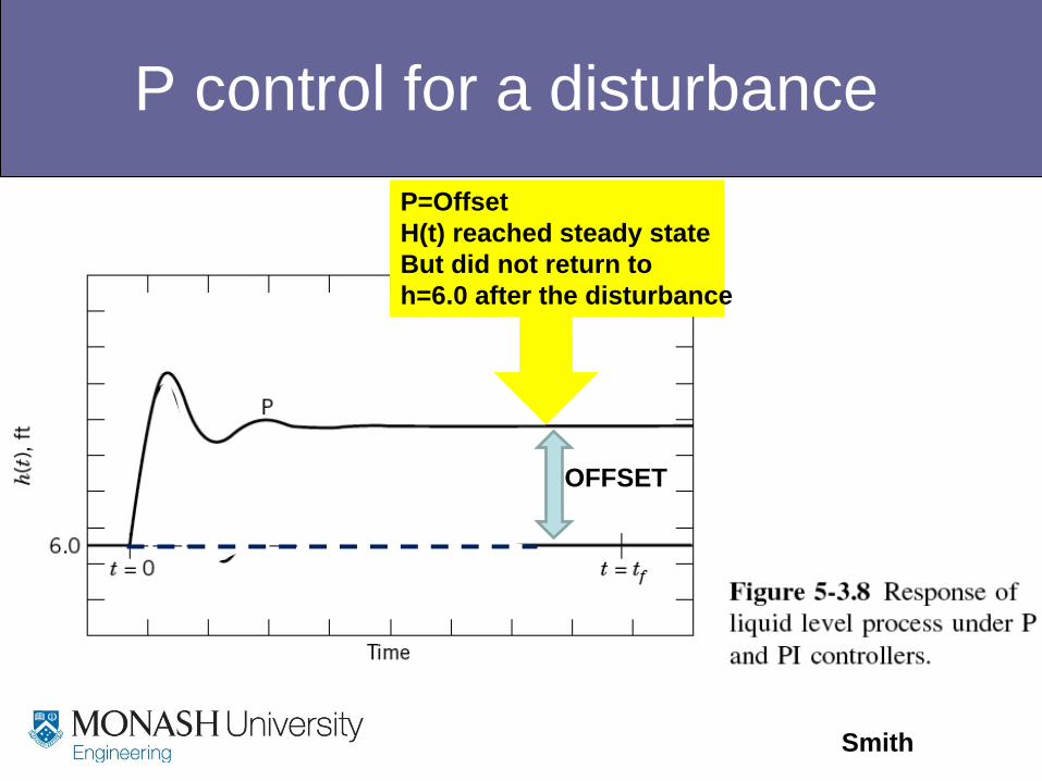
P control for a disturbance

Smith

P=Offset H(t) reached steady state But did not return to h=6.0 after the disturbance

OFFSET

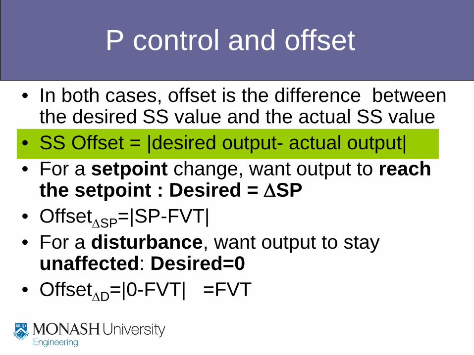
P control and offset

• In both cases, offset is the difference between the desired SS value and the actual SS value

• SS Offset = |desired output- actual output| • For a setpoint change, want output to reach

the setpoint : Desired = ∆SP • Offset∆SP=|SP-FVT| • For a disturbance, want output to stay

unaffected: Desired=0 • Offset∆D=|0-FVT| =FVT

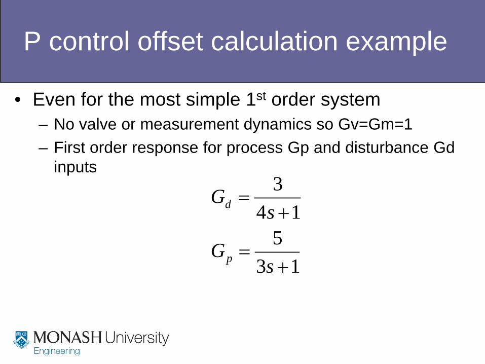
P control offset calculation example

• Even for the most simple 1st order system – No valve or measurement dynamics so Gv=Gm=1 – First order response for process Gp and disturbance Gd

inputs

135

143

+=

+=

sG

sG

p

d

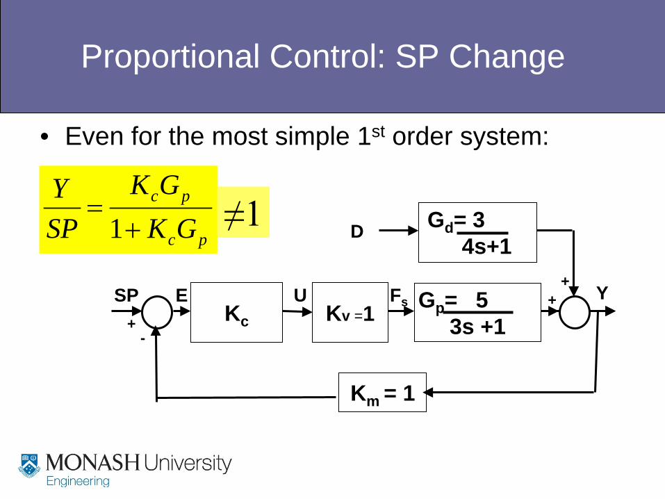
Proportional Control: SP Change

• Even for the most simple 1st order system:

pc

pc

GKGK

SPY

+=

1

Gp= 5 3s +1

Y Fs Kv =1 U

Km = 1

+ Kc

SP E +

-

Gd= 3 4s+1

D

+

≠1

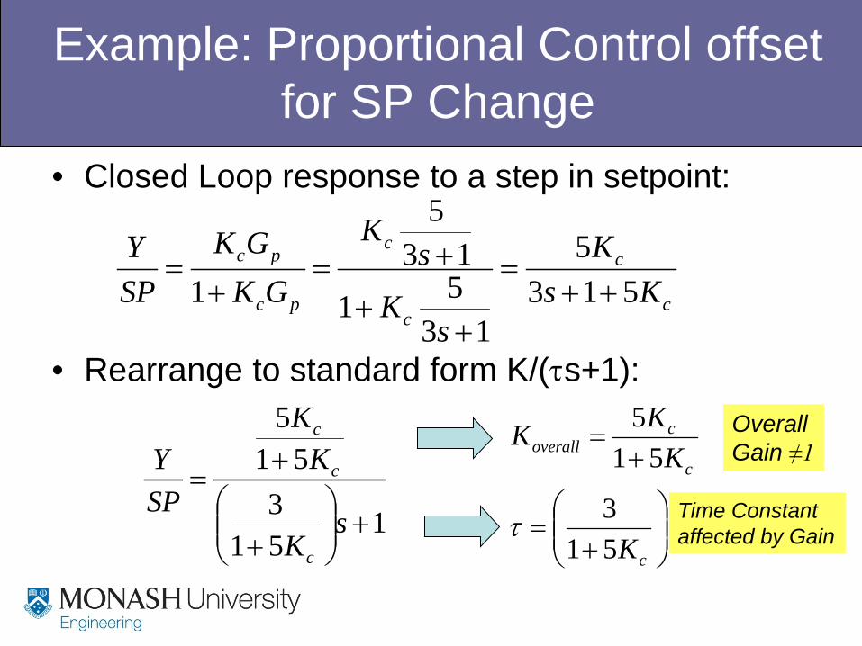
Example: Proportional Control offset for SP Change

• Closed Loop response to a step in setpoint:

• Rearrange to standard form K/(τs+1):

1513

515

+

+

+=

sK

KK

SPY

c

c

c

c

c

c

c

pc

pc

KsK

sK

sK

GKGK

SPY

5135

1351

135

1 ++=

++

+=+

=

+

=

+=

c

c

coverall

K

KKK

513

515

τ Time Constant affected by Gain

Overall Gain ≠1

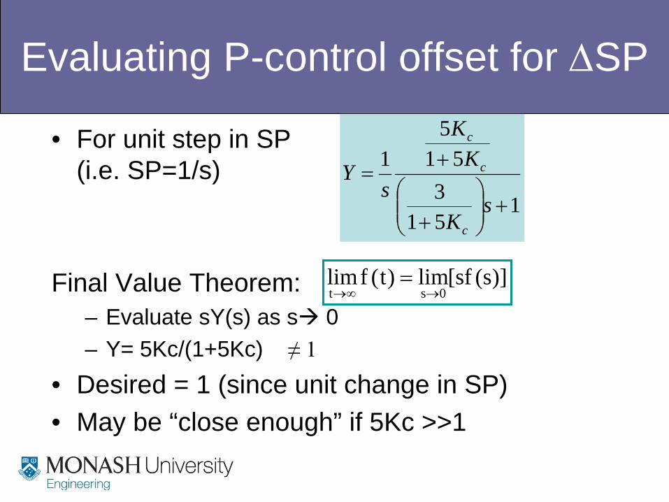
Evaluating P-control offset for ∆SP

• For unit step in SP (i.e. SP=1/s)

Final Value Theorem: – Evaluate sY(s) as s 0 – Y= 5Kc/(1+5Kc) ≠ 1

• Desired = 1 (since unit change in SP) • May be “close enough” if 5Kc >>1

1513

515

1

+

+

+=

sK

KK

sY

c

c

c

)]s(sf[lim)t(flim0st →∞→

=

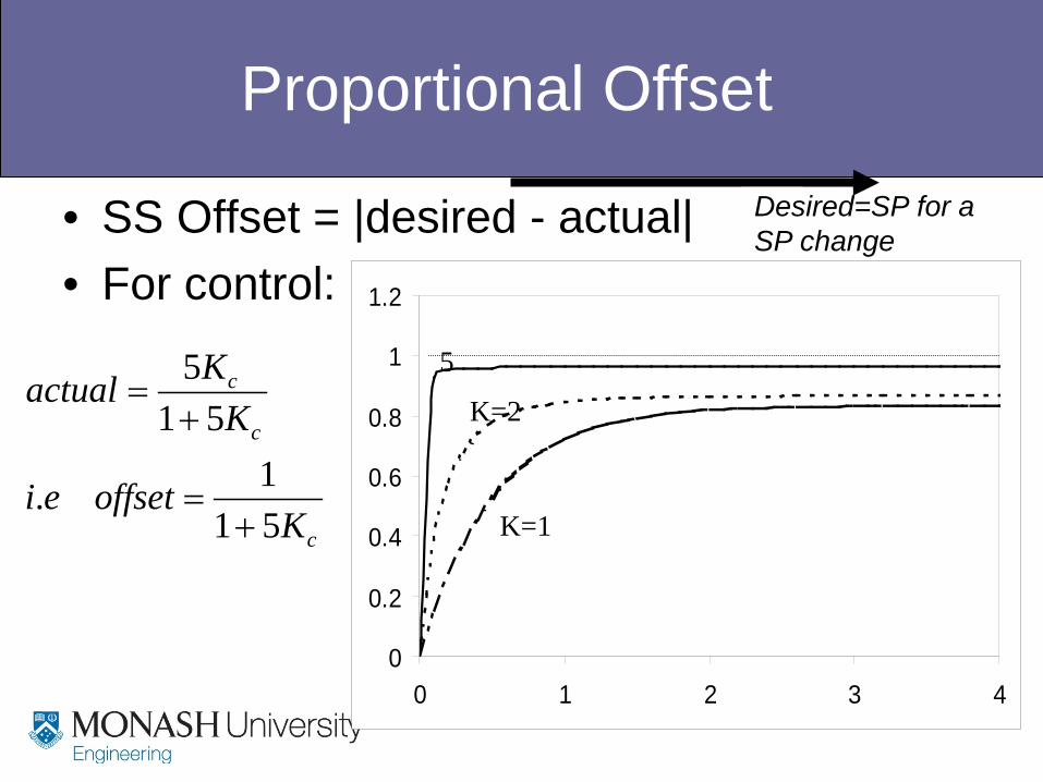
Proportional Offset

• SS Offset = |desired - actual| • For control:

c

c

c

Koffsetei

KKactual

511.

515

+=

+=

0

0.2

0.4

0.6

0.8

1

1.2

0 1 2 3 4

K=1

K=2

5

Desired=SP for a SP change

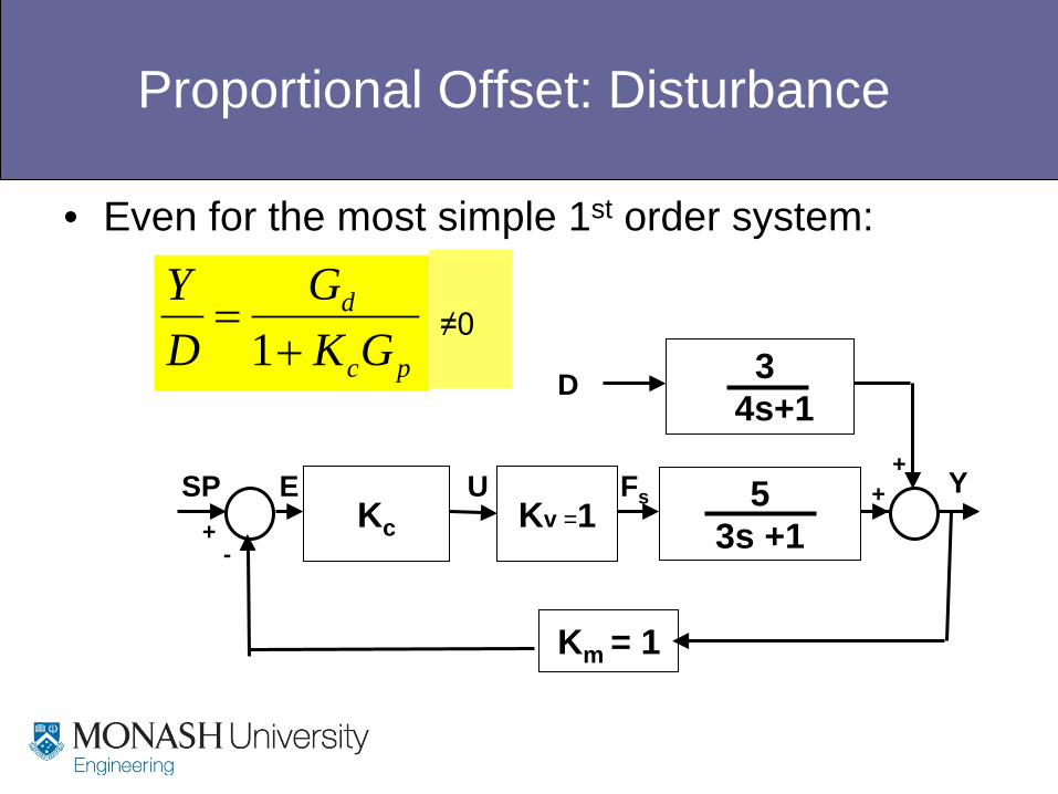
Proportional Offset: Disturbance

• Even for the most simple 1st order system:

5

3s +1 Y Fs Kv =1

U

Km = 1

+ Kc

SP E +

-

3

4s+1 D

+

pc

d

GKG

DY

+=

1 ≠0

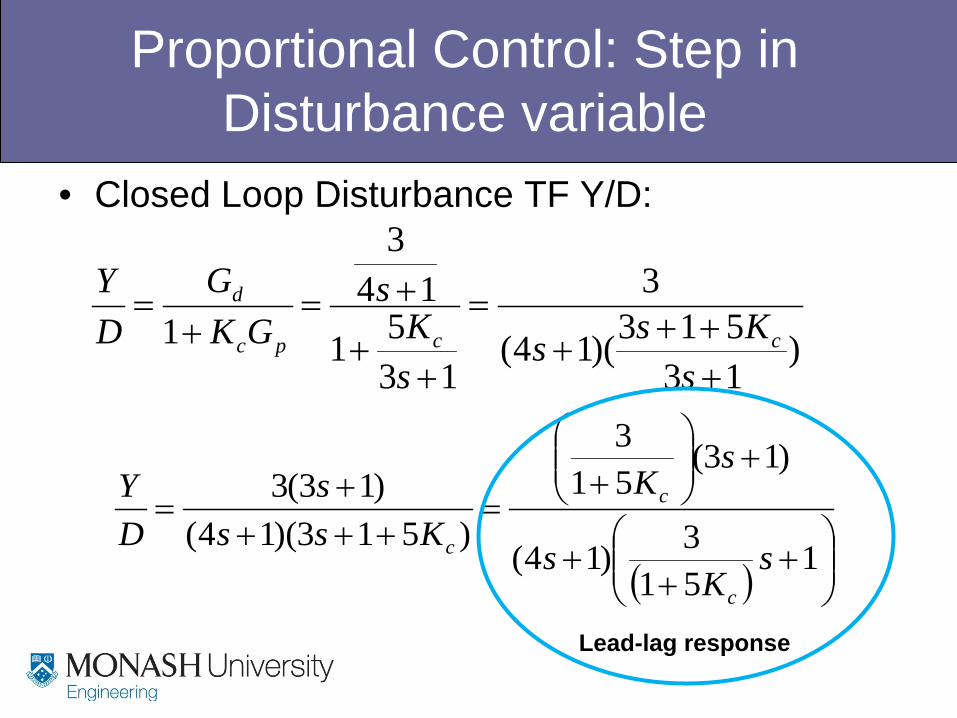
Proportional Control: Step in Disturbance variable

• Closed Loop Disturbance TF Y/D:

( )

+

++

+

+

=+++

+=

1513)14(

)13(513

)513)(14()13(3

sK

s

sK

Ksss

DY

c

c

c

)13513)(14(

3

1351

143

1+++

+=

++

+=+

=

sKss

sK

sGK

GDY

ccpc

d

Lead-lag response

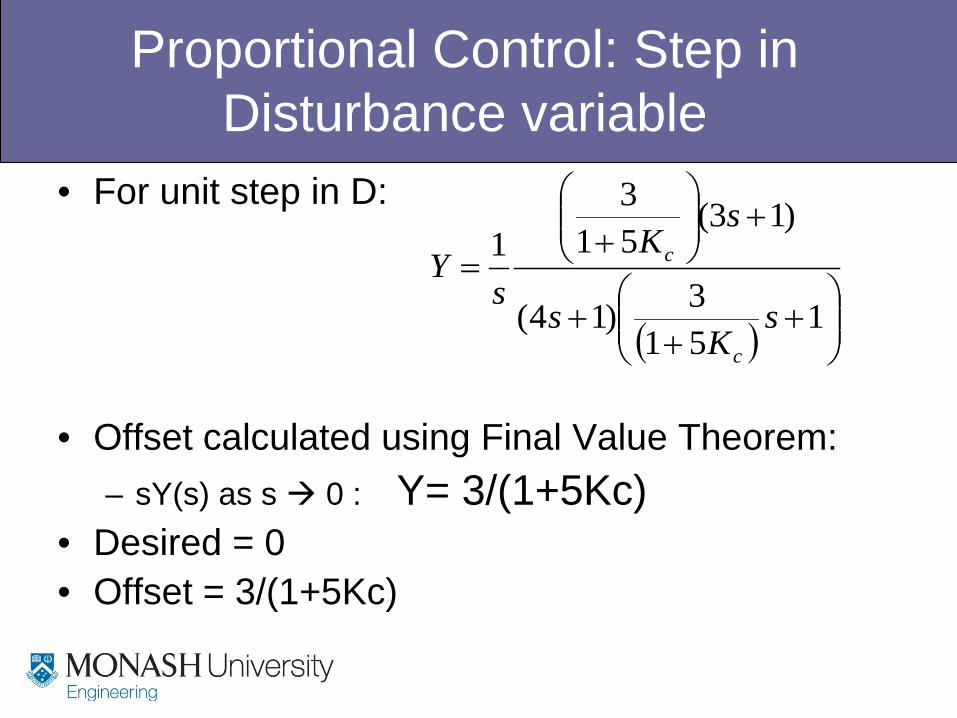
Proportional Control: Step in Disturbance variable

• For unit step in D:

• Offset calculated using Final Value Theorem: – sY(s) as s 0 : Y= 3/(1+5Kc)

• Desired = 0 • Offset = 3/(1+5Kc)

( )

+

++

+

+

=1

513)14(

)13(513

1

sK

s

sK

sY

c

c

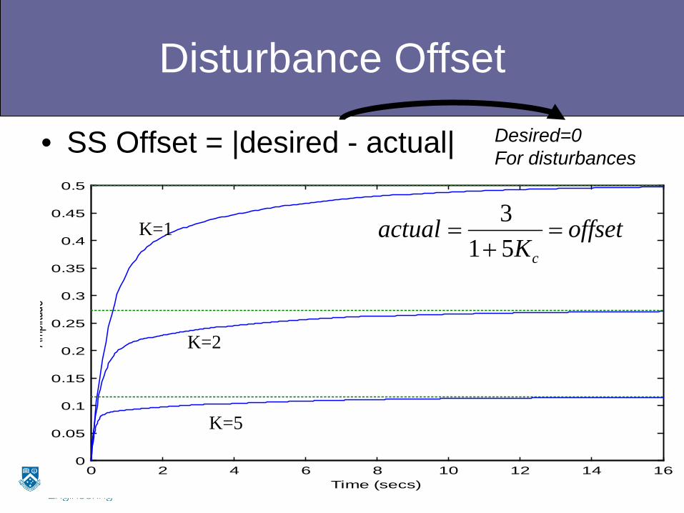
Disturbance Offset

• SS Offset = |desired - actual|

0 2 4 6 8 10 12 14 160

0.05

0.1

0.15

0.2

0.25

0.3

0.35

0.4

0.45

0.5

Time (secs)

Amplit

ude

K=1

K=2

K=5

offsetK

actualc

=+

=513

Desired=0 For disturbances

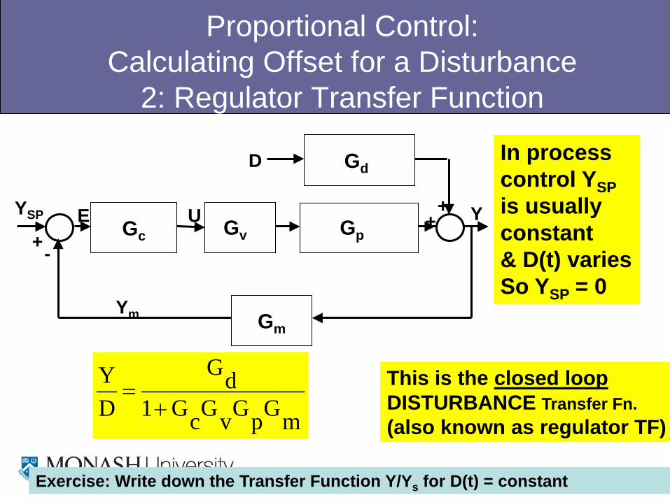
Proportional Control: Calculating Offset for a Disturbance

2: Regulator Transfer Function

Y Gc

U

Gm Ym

Gd D

+ + YSP E

+ - Gv Gp

In process control YSP is usually constant & D(t) varies So YSP = 0

mGpGvGcG1dG

DY

+= This is the closed loop

DISTURBANCE Transfer Fn. (also known as regulator TF)

Exercise: Write down the Transfer Function Y/Ys for D(t) = constant

Proportional control of 1st order

• Closed loop means offset is unavoidable • Offset may not be important in practice

– Or, the offset could be critical – This depends on the values of gains in the process

and the process application! • Offset occurs for both setpoint changes and

process disturbances • Controller Gain directly affects overall process

gain AND time constant

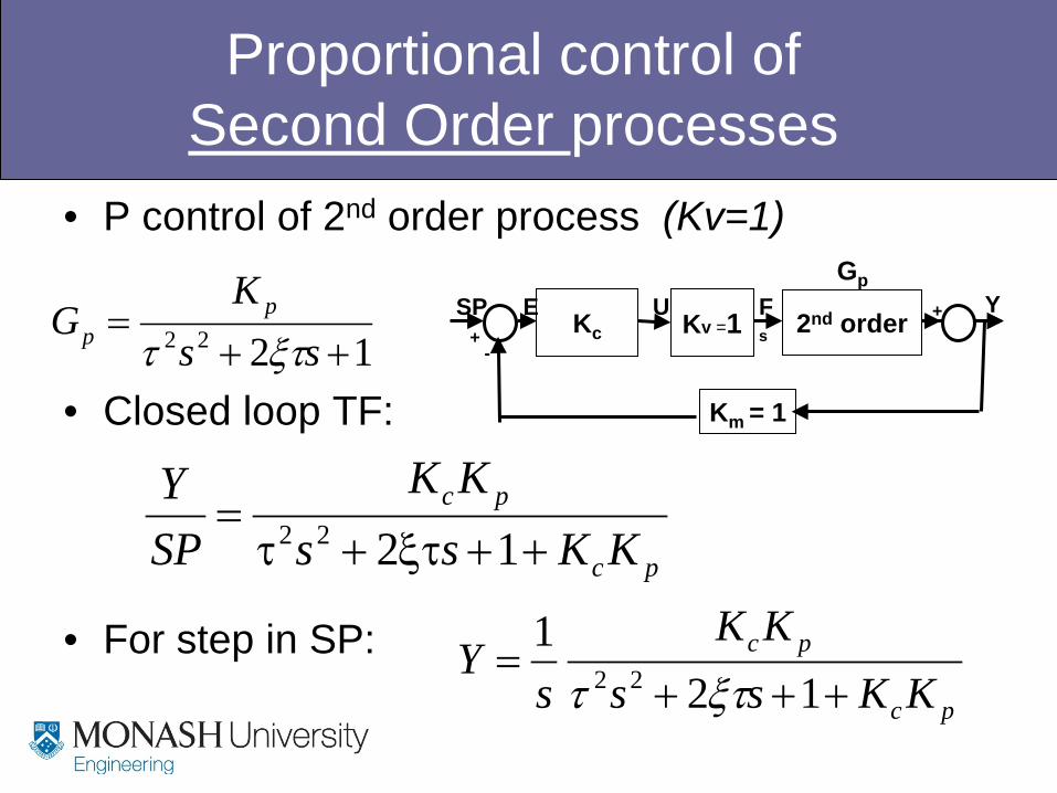
Proportional control of Second Order processes

• P control of 2nd order process (Kv=1)

• Closed loop TF:

• For step in SP:

1222 ++=

ssK

G pp ξττ

pc

pc

KKssKK

SPY

++ξτ+τ=

1222

2nd order Y F

s Kv =1 U

Km = 1

+ Kc SP E

+ -

Gp

pc

pc

KKssKK

sY

+++=

121

22 ξττ

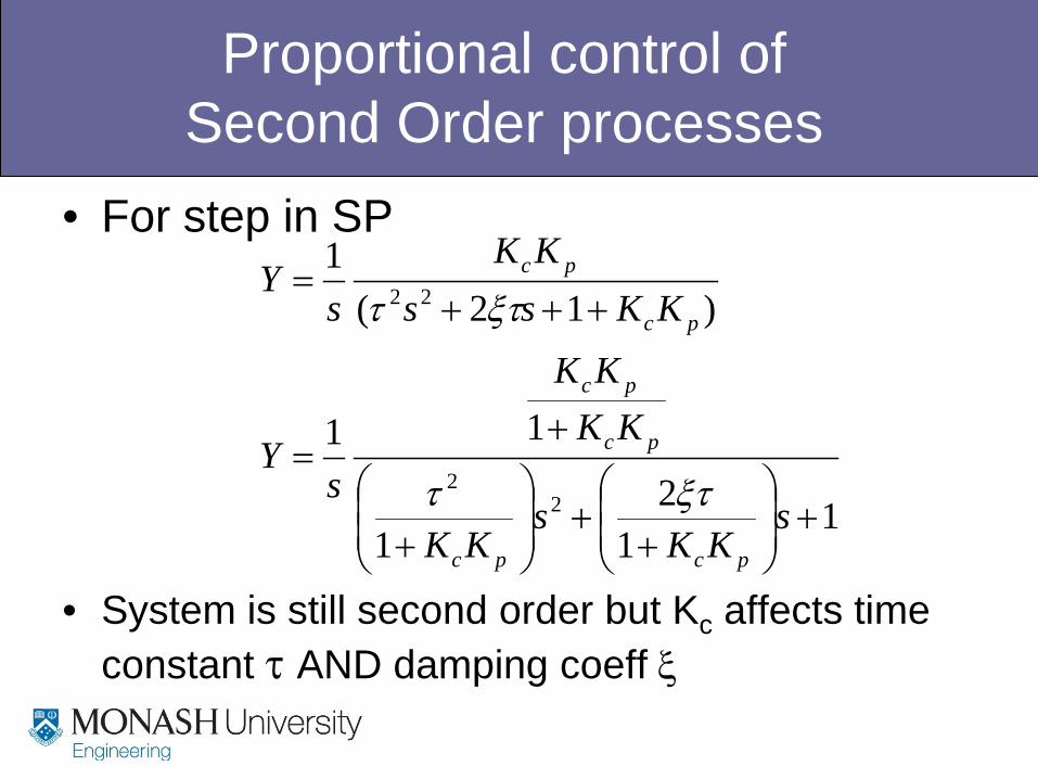
Proportional control of Second Order processes

• For step in SP

• System is still second order but Kc affects time constant τ AND damping coeff ξ

11

21

11

)12(1

22

22

+

++

+

+=

+++=

sKK

sKK

KKKK

sY

KKssKK

sY

pcpc

pc

pc

pc

pc

ξττ

ξττ

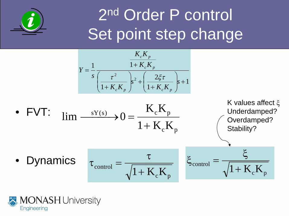
2nd Order P control Set point step change

• FVT:

• Dynamics

pc

pc)s(sY

KK1KK

0lim+

= →

pccontrol KK1+

τ=τ

pccontrol KK1+

ξ=ξ

11

21

11

22

+

++

+

+=

sKK

sKK

KKKK

sY

pcpc

pc

pc

ξττ

K values affect ξ Underdamped? Overdamped? Stability?

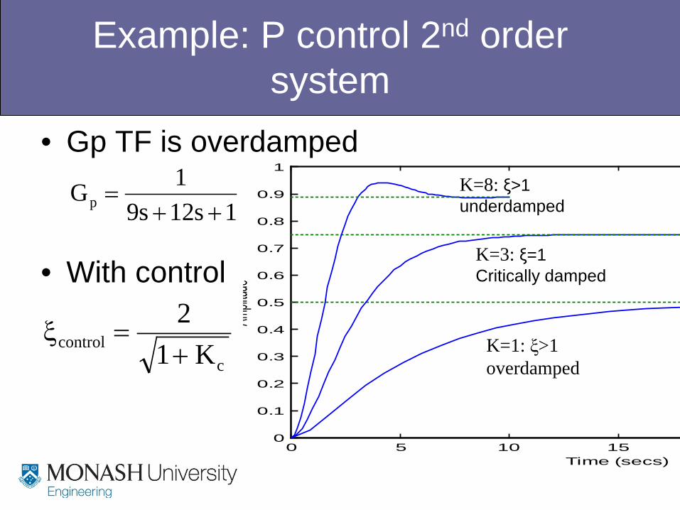
Example: P control 2nd order system

1s12s91Gp ++

=

ccontrol K1

2+

=ξ

0 5 10 150

0.1

0.2

0.3

0.4

0.5

0.6

0.7

0.8

0.9

1

Time (secs)

Amplitu

de

K=1: ξ>1 overdamped

K=3: ξ=1 Critically damped

K=8: ξ>1 underdamped

• Gp TF is overdamped

• With control

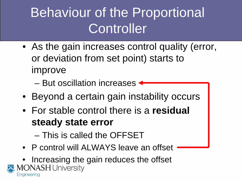
Behaviour of the Proportional Controller

• As the gain increases control quality (error, or deviation from set point) starts to improve – But oscillation increases

• Beyond a certain gain instability occurs • For stable control there is a residual

steady state error – This is called the OFFSET

• P control will ALWAYS leave an offset • Increasing the gain reduces the offset

P vs PI control

• Discussed P control – 1st and 2nd order processes – SP and D changes

• Always have offset for P control • Possible to change stability of loop by

choice of Kc • What about PI control??

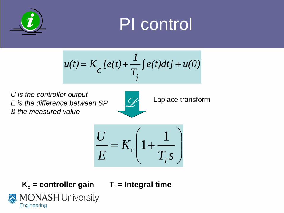
PI control

+=

sTK

EU

Ic

11

Laplace transform

∫ ++= u(0)e(t)dt]iT

1[e(t)cKu(t)

U is the controller output E is the difference between SP & the measured value

Kc = controller gain TI = Integral time

L

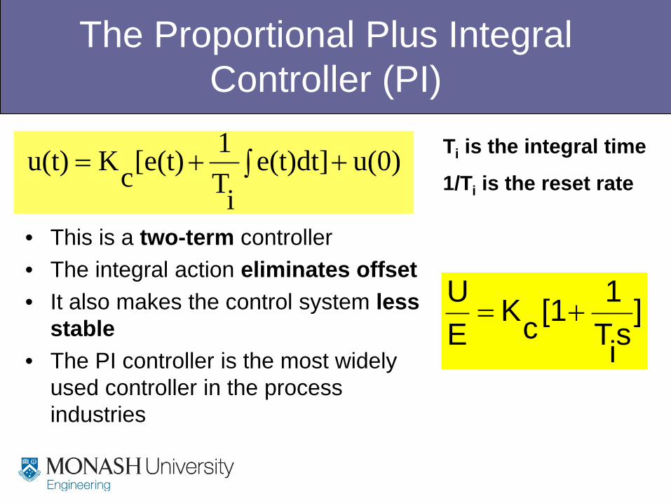
The Proportional Plus Integral Controller (PI)

• This is a two-term controller • The integral action eliminates offset • It also makes the control system less

stable • The PI controller is the most widely

used controller in the process industries

∫ ++= u(0)e(t)dt]iT

1[e(t)cKu(t)

]siT

1[1cKEU

+=

Ti is the integral time

1/Ti is the reset rate

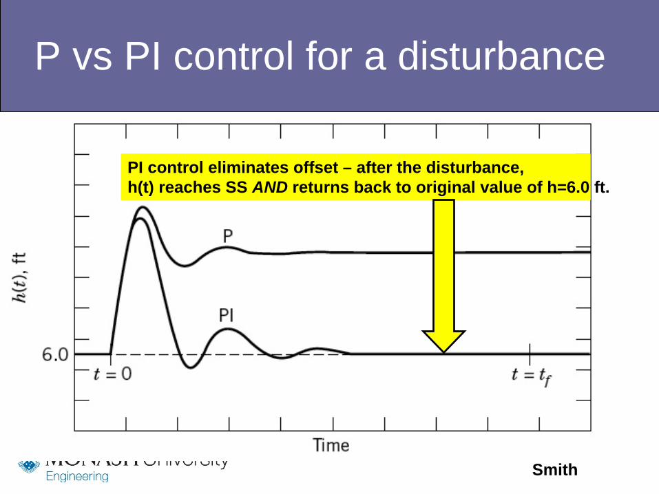
P vs PI control for a disturbance

Smith

PI control eliminates offset – after the disturbance, h(t) reaches SS AND returns back to original value of h=6.0 ft.

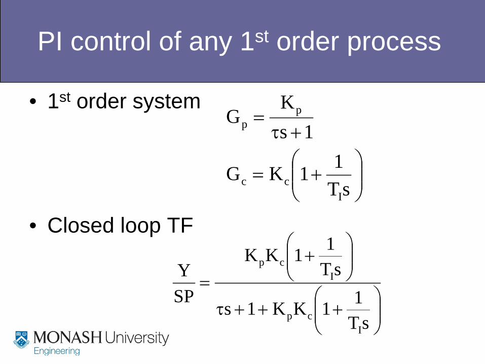
PI control of any 1st order process

• 1st order system

• Closed loop TF

+=

+τ=

sT11KG

1sK

G

Icc

pp

+++τ

+

=

sT11KK1s

sT11KK

SPY

Icp

Icp

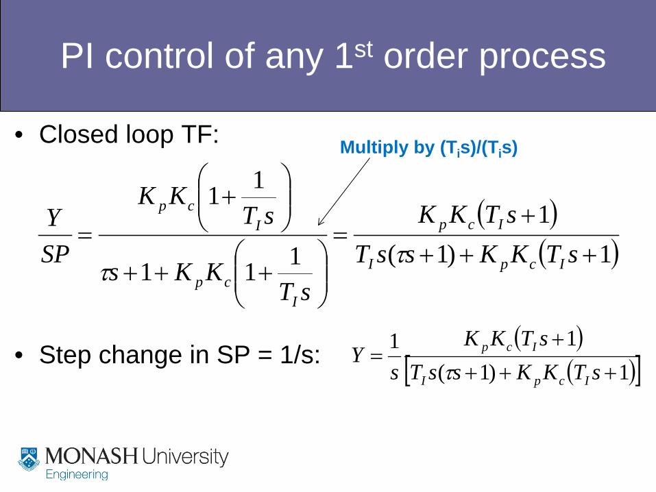
PI control of any 1st order process

• Closed loop TF:

• Step change in SP = 1/s:

( )( )1)1(1

111

11

+++

+=

+++

+

=sTKKssT

sTKK

sTKKs

sTKK

SPY

IcpI

Icp

Icp

Icp

ττ

( )( )[ ]1)1(11

+++

+=

sTKKssTsTKK

sY

IcpI

Icp

τ

Multiply by (Tis)/(Tis)

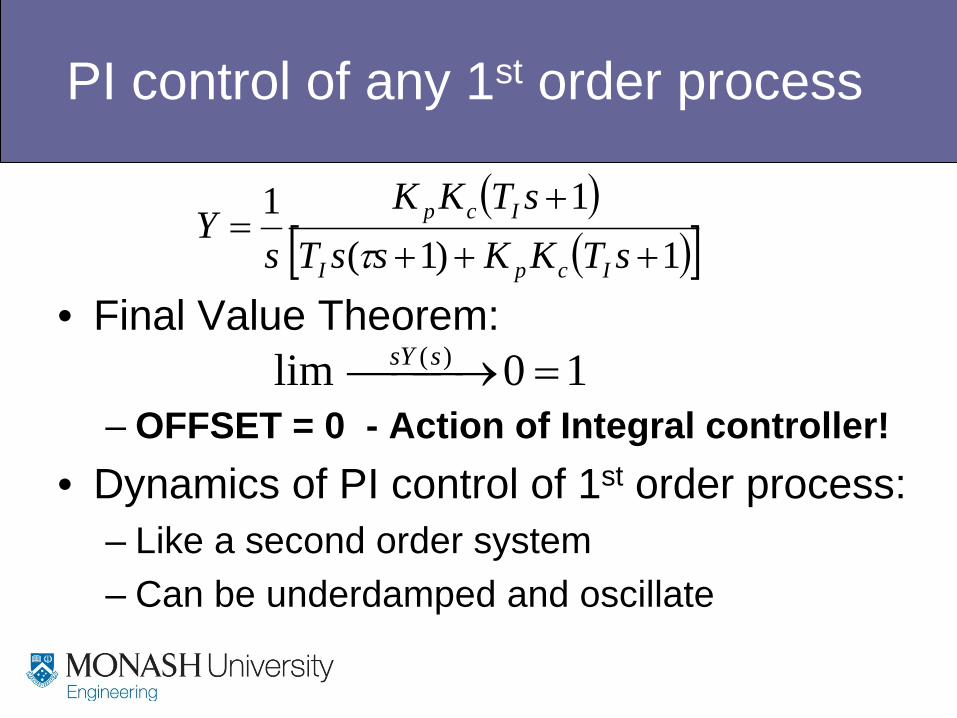
PI control of any 1st order process

• Final Value Theorem:

– OFFSET = 0 - Action of Integral controller! • Dynamics of PI control of 1st order process:

– Like a second order system – Can be underdamped and oscillate

10lim )( = → ssY

( )( )[ ]1)1(11

+++

+=

sTKKssTsTKK

sY

IcpI

Icp

τ

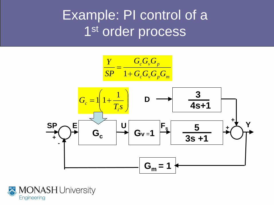
Example: PI control of a 1st order process

5

3s +1 Y Fs Gv =1

U

Gm = 1

+ Gc

SP E +

-

3

4s+1 D

+

mpvc

pvc

GGGGGGG

SPY

+=

1

+=

sTG

ic

111

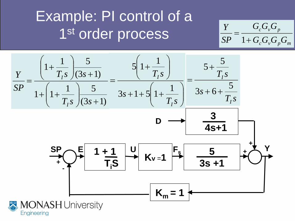
Example: PI control of a 1st order process

5

3s +1 Y Fs Kv =1

U

Km = 1

+ 1 + 1 TiS

SP E +

-

3

4s+1 D

+

mpvc

pvc

GGGGGGG

SPY

+=

1

)13(5111

)13(511

+

++

+

+

=

ssT

ssTSPY

I

I

+++

+

=

sTs

sT

I

I

11513

115

sTs

sT

I

I

563

55

++

+=

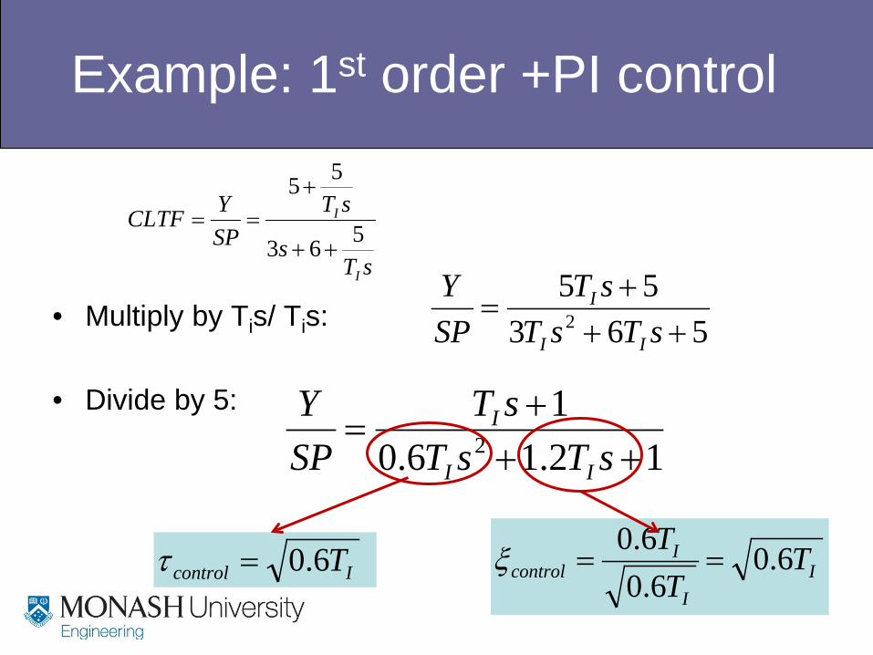
Example: 1st order +PI control

• Multiply by Tis/ Tis:

• Divide by 5:

56355

2 +++

=sTsT

sTSPY

II

I

Icontrol T6.0=τ II

Icontrol T

TT 6.06.0

6.0==ξ

12.16.01

2 +++

=sTsT

sTSPY

II

I

sTs

sTSPYCLTF

I

I

563

55

++

+==

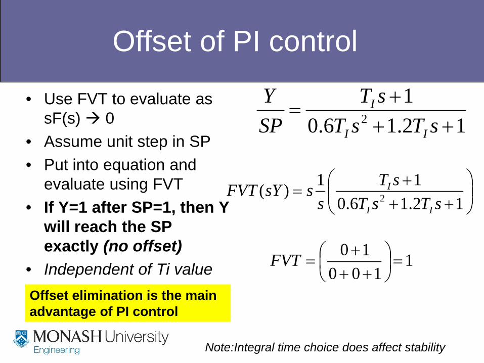
Offset of PI control

• Use FVT to evaluate as sF(s) 0

• Assume unit step in SP • Put into equation and

evaluate using FVT • If Y=1 after SP=1, then Y

will reach the SP exactly (no offset)

• Independent of Ti value

12.16.01

2 +++

=sTsT

sTSPY

II

I

++

+=

12.16.011)( 2 sTsT

sTs

ssYFVTII

I

1100

10=

+++

=FVT

Offset elimination is the main advantage of PI control

Note:Integral time choice does affect stability

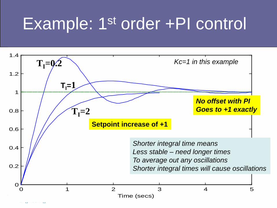
Example: 1st order +PI control

5sT6sT35sT5

SPY

I2

I

I

+++

=

0 1 2 3 4 50

0.2

0.4

0.6

0.8

1

1.2

1.4

Time (secs)

TI=2

TI=1

TI=0.2 Kc=1 in this example

Shorter integral time means Less stable – need longer times To average out any oscillations Shorter integral times will cause oscillations

Setpoint increase of +1

No offset with PI Goes to +1 exactly

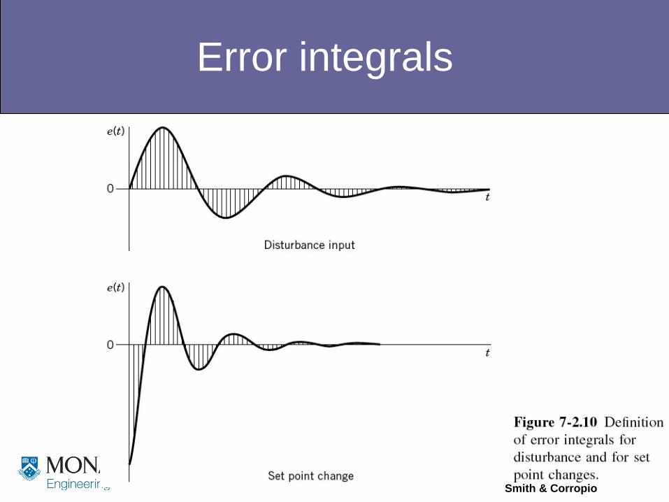
Error integrals

Smith & Corropio

P vs PI control for a disturbance

Smith

PI control eliminates offset – after the disturbance, h(t) reaches SS AND returns back to original value of h=6.0 ft.

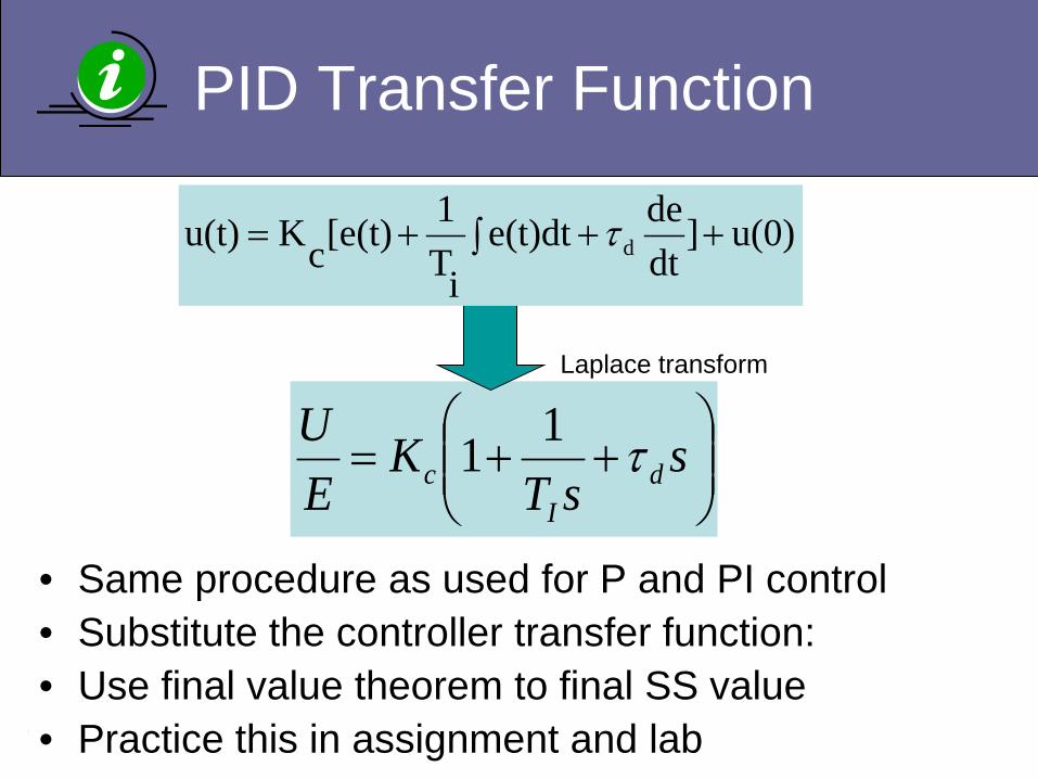
PID Transfer Function

• Same procedure as used for P and PI control • Substitute the controller transfer function: • Use final value theorem to final SS value • Practice this in assignment and lab

++= s

sTK

EU

dI

c τ11

Laplace transform

∫ +++= u(0)]dtdee(t)dt

iT1[e(t)cKu(t) dτ

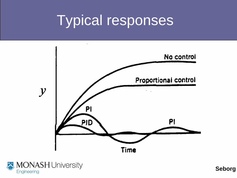
Typical responses

Seborg

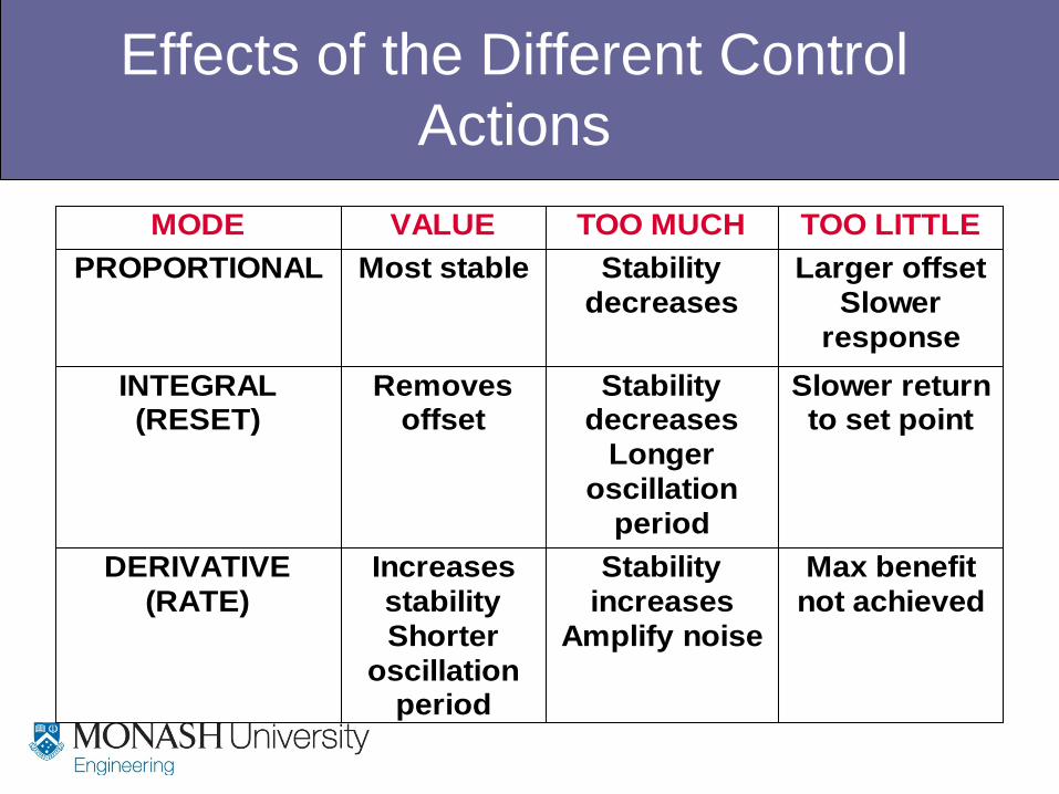
Effects of the Different Control Actions

MODE VALUE TOO MUCH TOO LITTLEPROPORTIONAL Most stable Stability

decreasesLarger offset

Slower response

INTEGRAL (RESET)

Removes offset

Stability decreases

Longer oscillation

period

Slower return to set point

DERIVATIVE (RATE)

Increases stability Shorter

oscillation period

Stability increases

Amplify noise

Max benefit not achieved

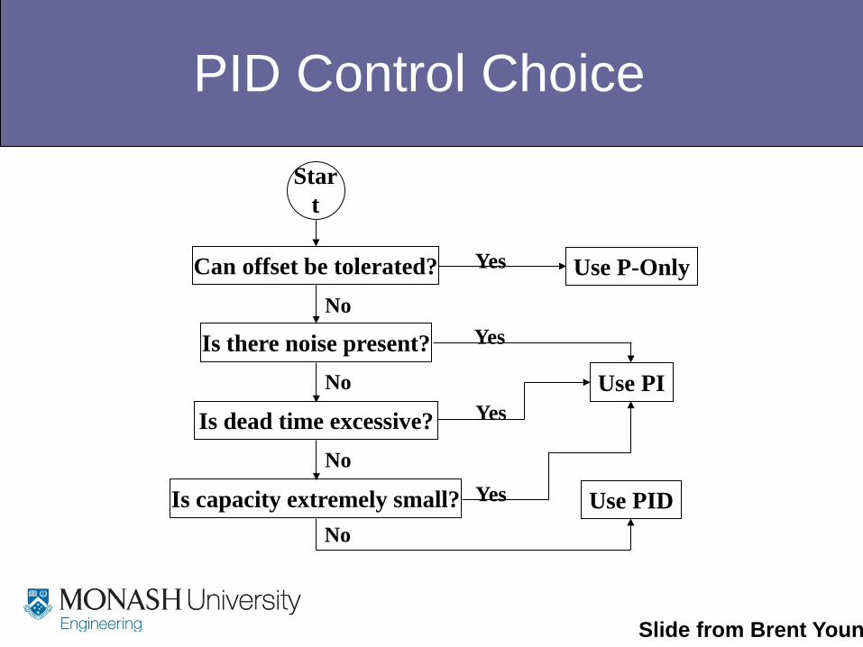
PID Control Choice

Start

Can offset be tolerated?

Is there noise present?

Is dead time excessive?

Is capacity extremely small? Use PID

Use PI

Use P-Only Yes

Yes

Yes

Yes

No

No

No

No

Slide from Brent Youn

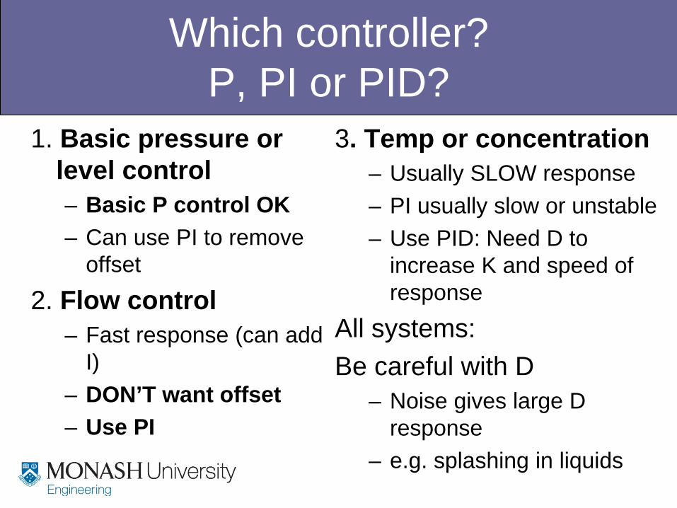
Which controller? P, PI or PID?

1. Basic pressure or level control – Basic P control OK – Can use PI to remove

offset 2. Flow control

– Fast response (can add I)

– DON’T want offset – Use PI

3. Temp or concentration – Usually SLOW response – PI usually slow or unstable – Use PID: Need D to

increase K and speed of response

All systems: Be careful with D

– Noise gives large D response

– e.g. splashing in liquids

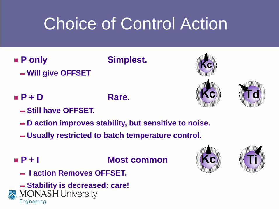
Choice of Control Action

P only Simplest. Will give OFFSET

P + D Rare. Still have OFFSET. D action improves stability, but sensitive to noise. Usually restricted to batch temperature control.

P + I Most common I action Removes OFFSET. Stability is decreased: care!

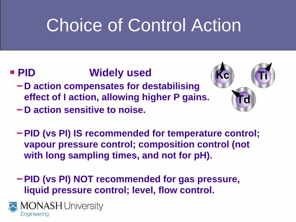
Choice of Control Action

PID Widely used D action compensates for destabilising effect of I action, allowing higher P gains. D action sensitive to noise. PID (vs PI) IS recommended for temperature control; vapour pressure control; composition control (not with long sampling times, and not for pH).

PID (vs PI) NOT recommended for gas pressure, liquid pressure control; level, flow control.

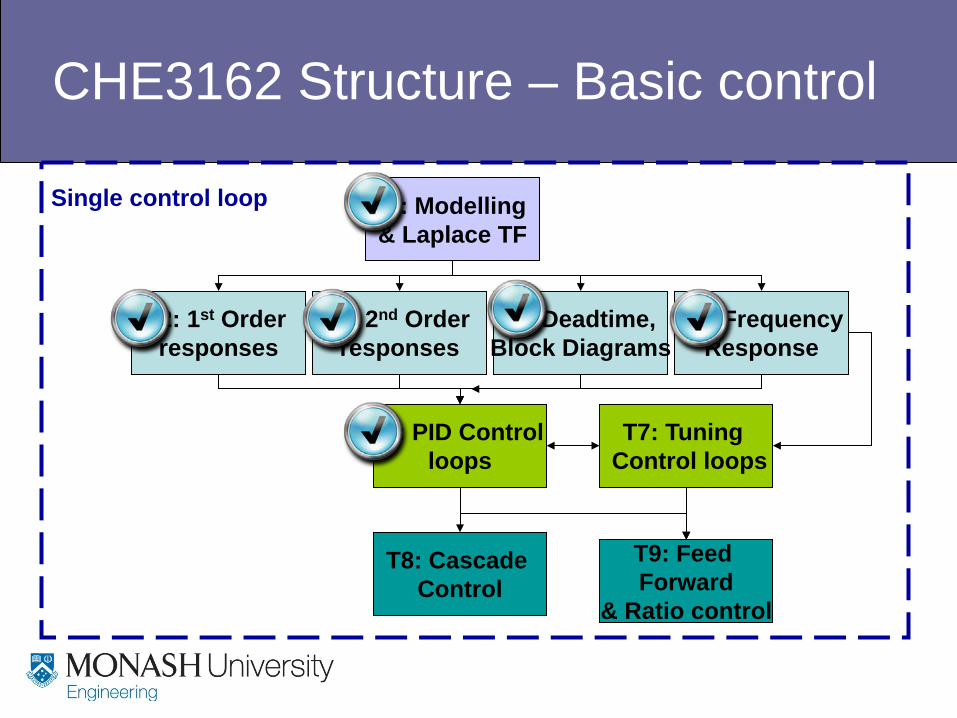
CHE3162 Structure – Basic control

T1: Modelling & Laplace TF

T2: 1st Order responses

T3: 2nd Order responses

T4: Deadtime, Block Diagrams

T5: Frequency Response

T6: PID Control loops

T7: Tuning Control loops

T8: Cascade Control

T9: Feed Forward

& Ratio control

Single control loop