![CMOS linear image sensor - Hamamatsu Photonics3 CMOS linear image sensor S13488 Electrical and optical characteristics [Ta=25 °C, Vdd=5 V, V(CLK)=V(ST)=5 V, f(CLK)=10 MHz] Parameter](https://static.fdocument.org/doc/165x107/60abeb8e2a5f391b163138b2/cmos-linear-image-sensor-hamamatsu-photonics-3-cmos-linear-image-sensor-s13488.jpg)
Characteristics of Linear System
42
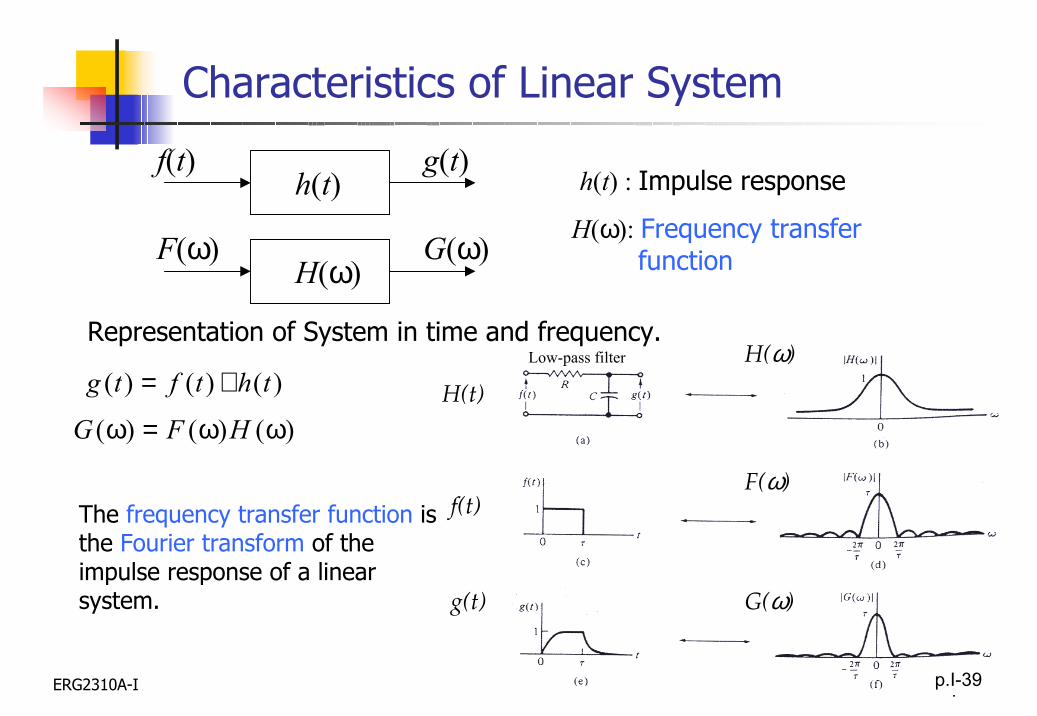
ERG2310A-I p. I-39 f(t) g(t) h(t) F(ω) G(ω) H(ω) ) ( ) ( ) ( t h t f t g ∗ = ) ( ) ( ) ( ω ω = ω H F G The frequency transfer function is the Fourier transform of the impulse response of a linear system. h(t) : Impulse response H(ω): Frequency transfer function Low-pass filter Representation of System in time and frequency. Characteristics of Linear System H(ω) F(ω) G(ω) H(t) f(t) g(t) p.I-39
Transcript of Characteristics of Linear System
ERG2310A-I p. I-39
f(t) g(t)h(t)
F(ω) G(ω)H(ω)
)()()( thtftg ∗=
)()()( ωω=ω HFG
The frequency transfer function is the Fourier transform of the impulse response of a linear system.
h(t) : Impulse response
H(ω): Frequency transferfunction
Low-pass filterRepresentation of System in time and frequency.
Characteristics of Linear System
H(ω)
F(ω)
G(ω)
H(t)
f(t)
g(t)
p.I-39
ERG2310A-I p. I-40
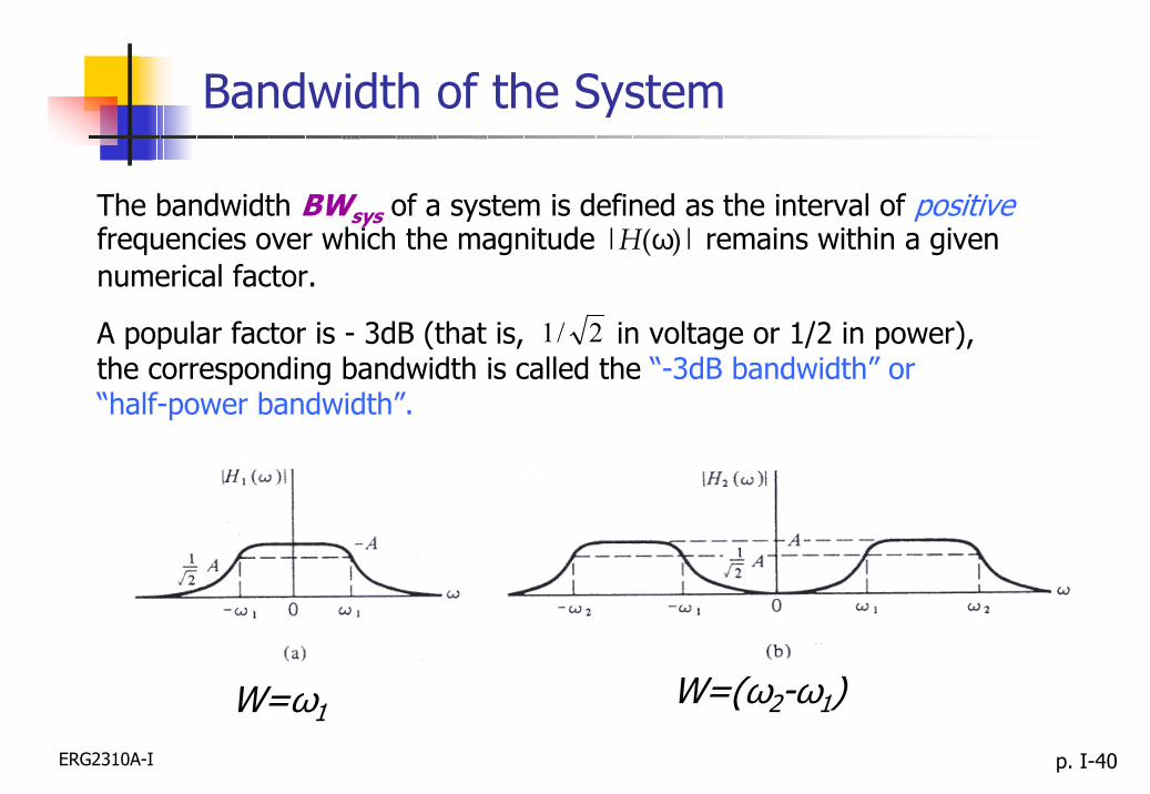
The bandwidth BWsys of a system is defined as the interval of positivefrequencies over which the magnitude |H(ω)| remains within a given numerical factor.
A popular factor is - 3dB (that is, in voltage or 1/2 in power),the corresponding bandwidth is called the “-3dB bandwidth” or“half-power bandwidth”.
2/1
Bandwidth of the System
W=ω1W=(ω2-ω1)

ERG2310A-I p. I-41
Bandwidth of the Signal
The bandwidth BWsig of a signal f(t) is defined as the range of positivefrequencies over which the magnitude |F(ω)| remains within a given numerical factor.
3-dB (or half-power) bandwidth: positive frequency range at which the amplitude spectrum |F(ω)| drops to a value equals to |F(ω)|/√2(or |F(ω)|2/2 in power).
A signal is called band-limited signal if |F(ω)| =0 for |ω | > ωM .
ERG2310A-I p. I-42
Distortionless Transmission
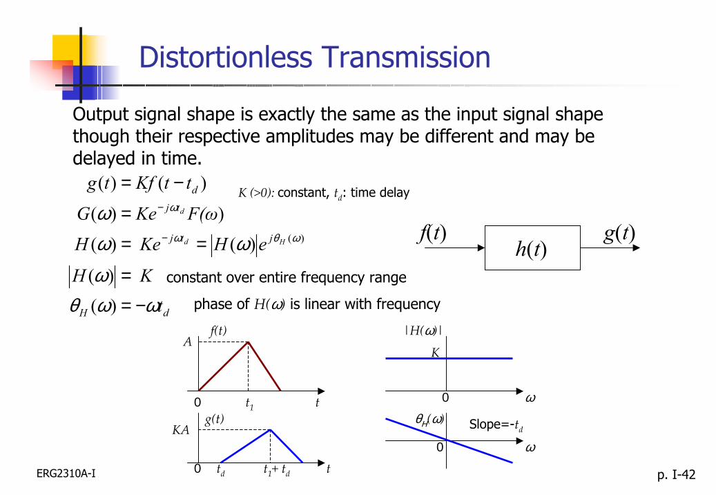
Output signal shape is exactly the same as the input signal shape though their respective amplitudes may be different and may be delayed in time.
)( )(
)( )(
))(
)()(
)(
dH
jtj
tjd
tKH
eHKeH
F(ωKeG
ttKftg
Hd
d
ωωθω
ωωω
ωθω
ω
−==
==
=
−=
−
−
f(t) g(t)h(t)
K (>0): constant, td: time delay
constant over entire frequency range
phase of H(ω) is linear with frequency
0 t1
0 td t1+ td
t
t
KA
Af(t)
g(t)
K
|H(ω)|
ω0
θΗ(ω)
ω0
Slope=-td

ERG2310A-I p. I-43
Distortionless Transmission
If K is not a constant (i.e. K is frequency dependent)
Frequency components of input signal are transmitted with different amount of gain / attenuation.
Amplitude distortion
If the phase of H(ω) is not linear with frequency
Frequency components of input signal are transmitted with different amount of time delay.
Phase distortion
Distorted output signal

ERG2310A-I p. I-44
Filters
After the input signal passes through the system, relative amplitudes of the frequency components in the input signal are changed or some of its frequency components are suppressed filtering (frequency-selective)
F(ω) G(ω)H(ω)
Transfer function (frequency response) H(ω) of a system acts as a filter on the input signal

ERG2310A-I p. I-45
Ideal Frequency-Selective Filters
Low-Pass
><
=c
cHωωωω
ω 0 1
)(
<<
=otherwise 0
1)( 21 ωωω
ωH
><
=c
cHωωωω
ω 1 0
)(
<<
=otherwise 1
0)( 21 ωωω
ωHBand-Stop
High-Pass
Band-Pass
−ω2 −ω1 0 ω1 ω2
ωc : cutoff frequency
−ωc 0 ωcω
|Η(ω) |−ωc 0 ωc
ω
|Η(ω) |
ω
|Η(ω) |
ω
|Η(ω) |
−ω2 −ω1 0 ω1 ω2
ERG2310A-I p. I-46
Non-ideal Frequency-Selective Filters
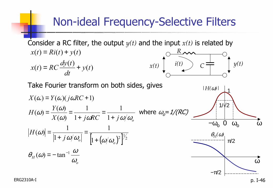
Consider a RC filter, the output y(t) and the input x(t) is related by
)()()(
)()()(
tydttdyRCtx
tytRitx
+=
+=
Take Fourier transform on both sides, gives
( )[ ]
oH
oo
o
jH
jRCjXYH
RCjYX
ωωωθ
ωωωωω
ωωωωωω
ωωω
1
212
tan)(
1
11
1)(
11
11
)()()(
)1)(()(
−−=
+=
+=
+=
+==
+=
where ωo=1/(RC)
x(t) y(t)C
R
i(t)
|H(ω)|
−ωo 0 ωo ωθH(ω)
π/2
−π/2
ω
1/√2
1
ERG2310A-I p. I-47
LTI System described by Differential Equations
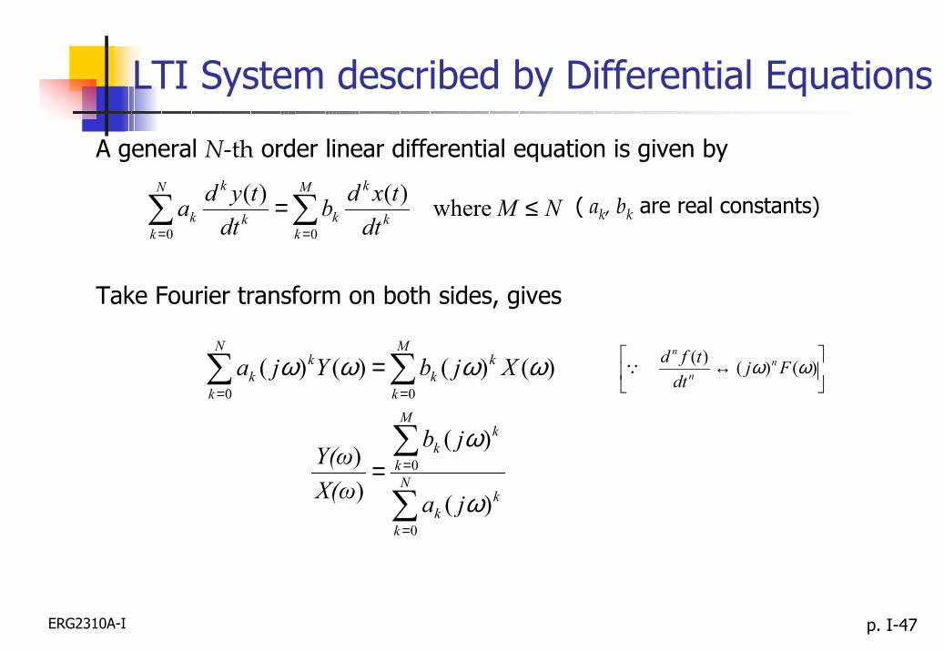
A general N-th order linear differential equation is given by
NMdttxdb
dttyda
M
kk
k
k
N
kk
k
k ≤=∑∑==
where)()(00
( ak, bk are real constants)
Take Fourier transform on both sides, gives
∑
∑
∑∑
=
=
==
=
=
N
k
kk
M
k
kk
M
k
kk
N
k
kk
ja
jb
X(ωY(ω
XjbYja
0
0
00
)(
)(
))
)()()()(
ω
ω
ωωωω
↔ )()()( ωω Fj
dttfd nn
n
Q

ERG2310A-I p. I-48
LTI System described by Differential Equations
Example: A system is described by y’(t)+2y(t)=x(t)+x’(t) . Determine the impulse response h(t).
)(')()(2)(' txtxtyty +=+
)()1()()2()()()(2)(
ωωωωωωωωωω
XjYjXjXYYj
+=++=+
ωωω
ωωω
jjj
XYH
+−=
++==
211
21
)()()(
Take Fourier transform on both sides, gives
↔ )()()( ωω Fj
dttfd nn
n
Q
Take Inverse Fourier transform on both sides, gives
)()()( 2 tuetth t−−=δ ( )
+
↔ωja
tue-at 1)( Q
<>
=0for 00for 1
)(tt
tu
ERG2310A-I p. I-49
LTI System described by Differential Equations
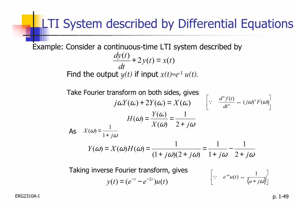
Example: Consider a continuous-time LTI system described by
)()(2)( txtydttdy =+
Find the output y(t) if input x(t)=e-1 u(t).
Take Fourier transform on both sides, gives)()(2)( ωωωω XYYj =+
ωωωω
jXYH
+==
21
)()()(
ωω
jX
+=
11)(
ωωωωωωω
jjjjHXY
+−
+=
++==
21
11
)2)(1(1)()()(
)()()( 2 tueety tt −− −=
As
Taking inverse Fourier transform, gives( )
+
↔ωja
tue-at 1)( Q
↔ )()()( ωω Fj
dttfd nn
n
Q
ERG2310A-I p. I-50
Parseval’s Theorem gives a relation between a time signal f(t)and its Fourier transform F(ω).
∫∫∞
∞−
∞
∞−ωω
π= .)(
21)( 22 dFdttf
where is the energy per unit of frequency normalized to a resistance of 1 ohm. It is called the energy spectral density of the signal f(t)
2)(ωF
• represents its energy per unit of frequency • displays the relative energy contributions of various frequency
components.
Energy Spectral Density
ERG2310A-I p. I-51
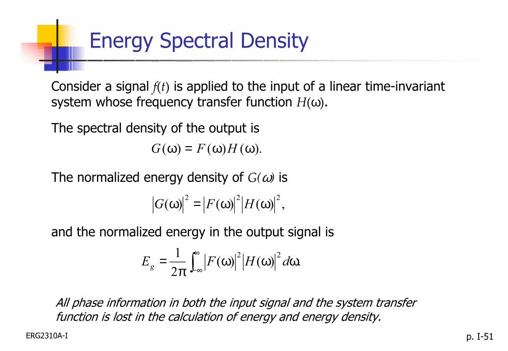
Consider a signal f(t) is applied to the input of a linear time-invariant system whose frequency transfer function H(ω).
The spectral density of the output is).()()( ωω=ω HFG
The normalized energy density of G(ω) is
,)()()( 222 ωω=ω HFG
and the normalized energy in the output signal is
∫∞
∞−ωωω
π= .)()(
21 22 dHFEg
All phase information in both the input signal and the system transfer function is lost in the calculation of energy and energy density.
Energy Spectral Density
ERG2310A-I p. I-52
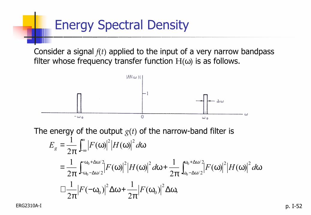
Consider a signal f(t) applied to the input of a very narrow bandpass filter whose frequency transfer function H(ω) is as follows.
The energy of the output g(t) of the narrow-band filter is
,)(21)(
21
)()(21)()(
21
)()(21
20
20
2/
2/
222/
2/
22
22
0
0
0
0
ω∆ωπ
+ω∆ω−π
≅
ωωωπ
+ωωωπ
=
ωωωπ
=
∫∫
∫ω∆+ω
ω∆−ω
ω∆+ω−
ω∆−ω−
∞
∞−
FF
dHFdHF
dHFEg
Energy Spectral Density
ERG2310A-I p. I-53
If the signal f(t) is real-valued [ f*(t) = f(t) ], then
)()(* ω=ω− FFand thus
)()( ω=ω− FF
Therefore,ω∆ω
π≅ 2
0 )(1 FEg
Note:Half of energy is contributed by the negative frequency components andhalf by the positive frequency components if the signal is real-valued.
Energy Spectral Density
,)(21)(
21 2
02
0 ωωπ
ωωπ
∆+∆−≅ FFEg

ERG2310A-I p. I-54
The energy spectral density can be measured by a device called a“multi-channel spectrum analyzer”.
Note:The area under the energy spectral density gives the energy within agiven band of frequencies.
Energy Spectral Density: Measurement

ERG2310A-I p. I-55
A signal is applied to the input of a low-pass filter with a magnitude frequency transfer function . Determine the required relations between the constants a, b such that exactly 50% of the input signal energy, on a 1-ohm basis, is transferred to the output.
)()( tuetf at−=22/)( bbH +ω=ω
Solution:The energy in the input signal f(t) is (across 1 ohm)
.21)(
0
22
adtedttfE at
f === ∫∫∞ −∞
∞−
The energy in the output signal g(t) is (across 1 ohm)
.))((
))((21
)()(21)(
21
0 2222
2
2222
2
222
∫
∫
∫ ∫
∞
∞
∞−
∞
∞−
∞
∞−
+ω+ωω
π=
ω+ω+ωπ
=
ωωωπ
=ωωπ
=
badb
dba
b
dHFdGEg
Energy Spectral Density: Example

ERG2310A-I p. I-56
Using a table of integrals,
.)(2)(2
2
baab
baabbEg +
=+
ππ
=
Since we require
fg EE 21=
so that
.21
21
)(2 abaab =+
Solving it, we find that the required relation is .ba =
Energy Spectral Density: Example
ERG2310A-I p. I-57
The time-averaged power of a signal is given by
∫−∞→=
2/
2/
2 .)(1limT
TTdttf
TP assuming a 1-ohm resistance.
This quantity is called the mean-square value of the signal f(t), designated simply as .)(2 tf
Let’s define a function called the power spectral density function, Sf(ω), where
∫∞
∞−
∆ωω
π= .)(
21 dSP f
The power spectral-density function Sf(ω) is in units of power (i.e. watts) per Hz. It describes the distribution of power versus frequency.
Power Spectral Density

ERG2310A-I p. I-58
Assuming f(t) is finite over the interval (-T/2, T/2). Then the truncated function f(t)rect(t/T) has finite energy and its Fourier transform is
)}./(rect)({)( TttfFT ℑ=ω
Parseval’s theorem for this truncated function is
∫ ∫−
∞
∞−ωω
π=
2/
2/
22 .)(21)(
T
T T dFdttf
Power Spectral Density

ERG2310A-I p. I-59
Thus, we have
∫ ∫−
∞
∞−∞→∞→ωω
π==
2/
2/
22 .)(211lim)(1lim
T
T TTTdF
Tdttf
TP
Hence the average power P across a 1-ohm resistor is given by
.)(211lim)(
21 2
∫∫∞
∞−∞→
∞
∞−ωω
π=ωω
πdF
TdS TTf
Power Spectral Density
.)(
lim)(2
TF
S T
Tf
ω=ω
∞→
ERG2310A-I p. I-60
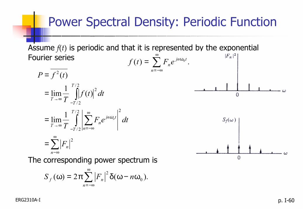
Assume f(t) is periodic and that it is represented by the exponential Fourier series ∑
∞
−∞=
ω=n
tjnneFtf .)( 0
∑
∫ ∑
∫
∞
∞−
−
∞
−∞=∞→
−∞→
=
=
=
=
nn
T
T n
tjnnT
T
TT
F
dteFT
dttfT
tfP
o
2
2/
2/
2
2/
2/
2
2
1lim
)(1lim
)(
ω
The corresponding power spectrum is
∑∞
−∞=
ω−ωδπ=ωn
nf nFS ).(2)( 02
Power Spectral Density: Periodic Function
ERG2310A-I p. I-61
Develop an expression for the power spectral density of
),/(rect)exp()( 0 TttjAtf ω=
both for finite T and as T → ∞.
Solution:From table, we have
).2/(Sa )}/(rect { TTATtA ω=ℑ
Using the frequency translation property of the Fourier transform, we get
].2/)(Sa[ )}/(rect )exp( { 00 TTATttjA ωωω −=ℑ
Thus, for a finite observation interval T, we have
].2/)[(Sa)(
)( 022
2
TTAT
FS Tf ω−ω=
ω≈ω
Power Spectral Density:Example

ERG2310A-I p. I-62
As the observation interval is made increasingly longer, the Sa2( ) pattern becomes more and more concentrated about ω = ω0 and in the limit,
).(2
]2/)[(Sa2
lim2
]}2/)[(Sa{lim)(
lim
02
022
022
2
ω−ωδπ=
ω−ω
ππ=
ω−ω=ω
∞→
∞→∞→
A
TTA
TTAT
F
T
T
T
T
Power Spectral Density:Example
ERG2310A-I p. I-63
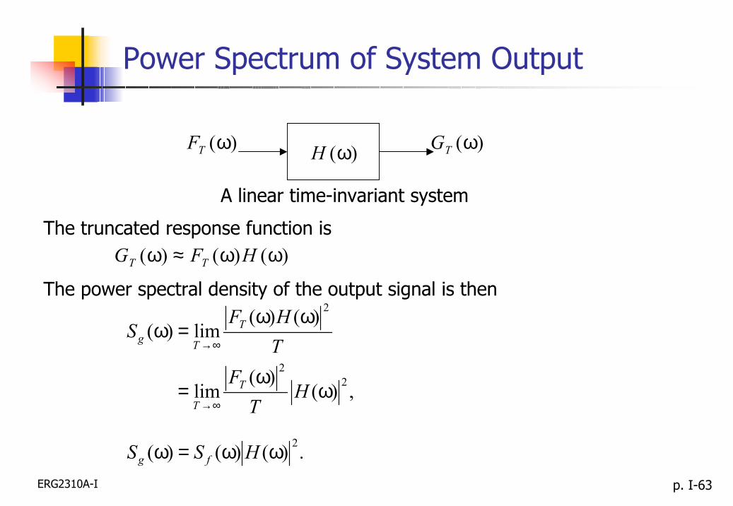
)(ωTF )(ωH )(ωTG
)()()( ωω≈ω HFG TT
A linear time-invariant system
The truncated response function is
The power spectral density of the output signal is then
,)()(
lim
)()(lim)(
22
2
ωω
=
ωω=ω
∞→
∞→
HT
FTHF
S
T
T
T
Tg
.)()()( 2ωω=ω HSS fg
Power Spectrum of System Output

ERG2310A-I p. I-64
The average power in the output signal is given by
.)()(21 2 ωωωπ
= ∫∞
∞−dHSP fg
Note that all phase information in both the input signal and the system transfer function is lost.
Average Power of System Output

ERG2310A-I p. I-65
The inverse Fourier transform of Sf(t) is called the autocorrelation function Rf(τ) of f(t).
∫
∫ ∫
∫ ∫∫
∫ ∫∫
∫
∫
−∞→
− −∞→
−
∞
∞−
+−
−∞→
∞
∞− −−∞→
∞
∞−∞→
∞
∞− ∞→
−
+=
+−=
=
=
=
=
ℑ=
2/
2/
*
2/
2/ 11
2/
2/ 1*
2/
2/ 1)(2/
2/ 1*
2/
2/ 11*2/
2/
*
*
2
1
)()(1lim
)()()(1lim
21)()(1lim
)()(2
1lim
)()(2
1lim
)(1lim21
)}({)(
1
1
T
TT
T
T
T
TT
T
T
ttjT
TT
jT
T
tjT
T
tj
T
jTTT
jTT
ff
dttftfT
dtdttttftfT
dtdtdetftfT
dedtetfdtetfT
deFFT
deFT
SR
τ
τδ
ωπ
ωπ
ωωωπ
ωωπ
ωτ
τω
ωτωω
ωτ
ωτ
Autocorrelation
}{ )( )( τω ff RS ℑ=
ERG2310A-I p. I-66
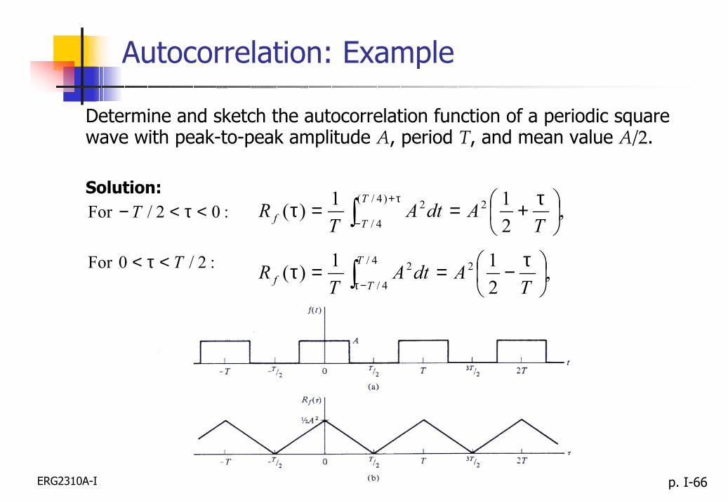
Determine and sketch the autocorrelation function of a periodic square wave with peak-to-peak amplitude A, period T, and mean value A/2.
Solution::02/For <τ<−T ∫
τ+
−
τ+==τ
)4/(
4/
22 ,211)(
T
Tf TAdtA
TR
:2/0For T<τ< ∫ −τ
τ−==τ
4/
4/
22 ,211)(
T
Tf TAdtA
TR
Autocorrelation: Example
ERG2310A-I p. I-67
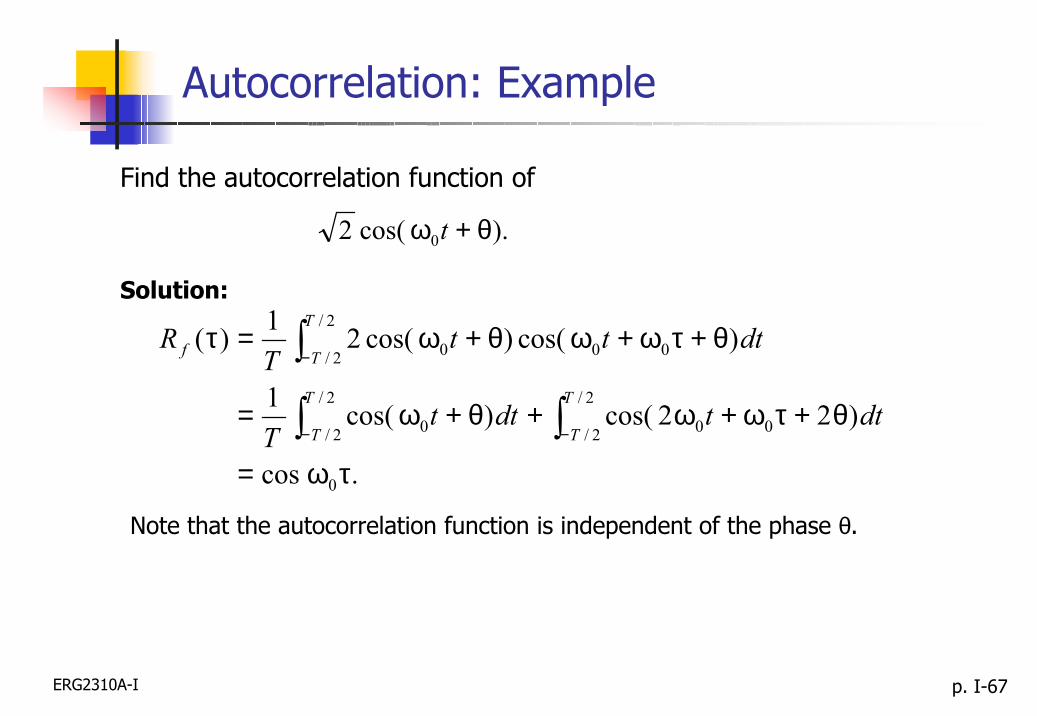
Find the autocorrelation function of
).cos(2 0 θ+ω t
Solution:
.cos
)22cos()cos(1
)cos()cos(21)(
0
2/
2/ 00
2/
2/ 0
2/
2/ 000
τω=
θ+τω+ω+θ+ω=
θ+τω+ωθ+ω=τ
∫∫
∫
−−
−
T
T
T
T
T
Tf
dttdttT
dtttT
R
Note that the autocorrelation function is independent of the phase θ.
Autocorrelation: Example

ERG2310A-I p. I-68
Detect or recognize signals that are masked by additive noise.
Drawbacks: Presence of noise in the output and lost of relative time shift.
Autocorrelation: Application
ERG2310A-I p. I-69
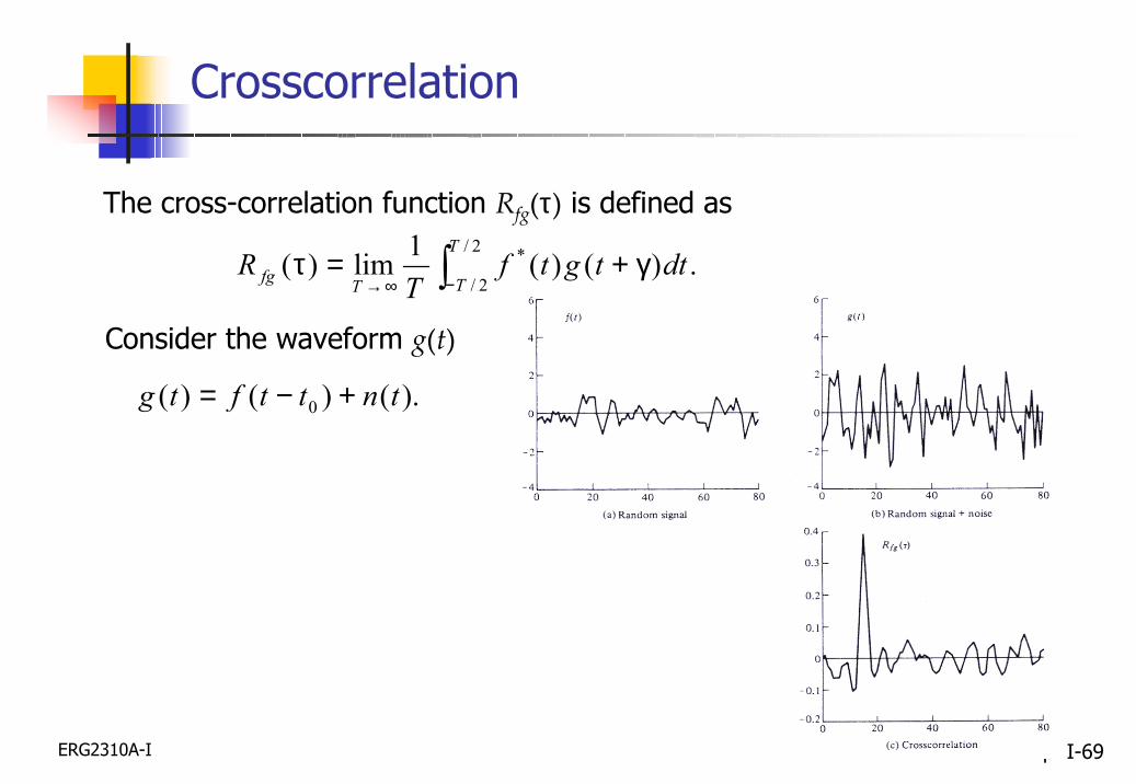
The cross-correlation function Rfg(τ) is defined as
∫−∞→γ+=τ
2/
2/
* .)()(1lim)(T
TTfg dttgtfT
R
Consider the waveform g(t)
).()()( 0 tnttftg +−=
Crosscorrelation
ERG2310A-I p. I-70
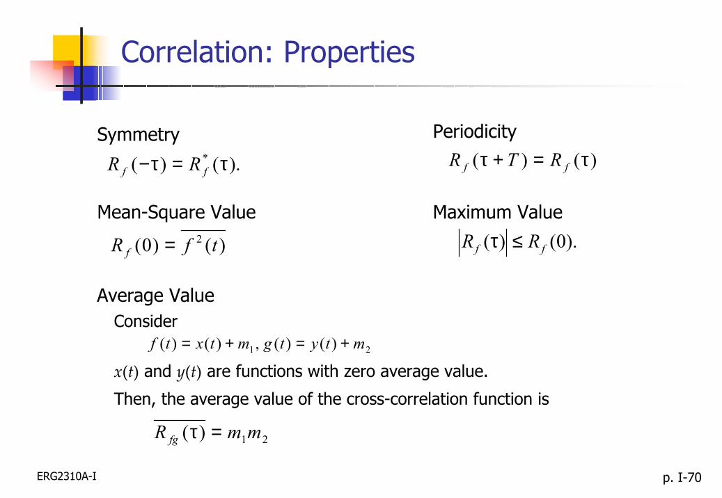
Symmetry
).()( * τ=τ− ff RR
Mean-Square Value
)()0( 2 tfR f =
Periodicity)()( τ=+τ ff RTR
Maximum Value
).0()( ff RR ≤τ
Average Value
21 )()( ,)()( mtytgmtxtf +=+=
21)( mmR fg =τ
Consider
x(t) and y(t) are functions with zero average value.
Then, the average value of the cross-correlation function is
Correlation: Properties
ERG2310A-I p. I-71
Additivity
)()()( tytxtz +=
).()()()(
)]()()][()([1lim)(2/
2/
**
τ+τ+τ+τ=
τ++τ++=τ ∫−∞→
yxxyyx
T
TTz
RRRR
dttytxtytxT
R
If x(t) and y(t) are uncorrelated,
).()()( τ+τ=τ yxz RRR
Consider
The corresponding autocorrelation function is
Correlation: Properties
ERG2310A-I p. I-72
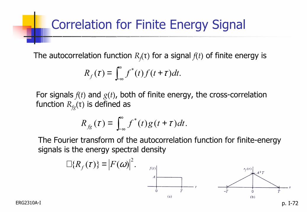
The autocorrelation function Rf(τ) for a signal f(t) of finite energy is
∫∞
∞−+= .)()()( * dttftfRf ττ
For signals f(t) and g(t), both of finite energy, the cross-correlation function Rfg(τ) is defined as
∫∞
∞−+= .)()()( * dttgtfR fg ττ
The Fourier transform of the autocorrelation function for finite-energy signals is the energy spectral density
.)()}({ 2ωτ FRf =ℑ
Correlation for Finite Energy Signal
ERG2310A-I p. I-73
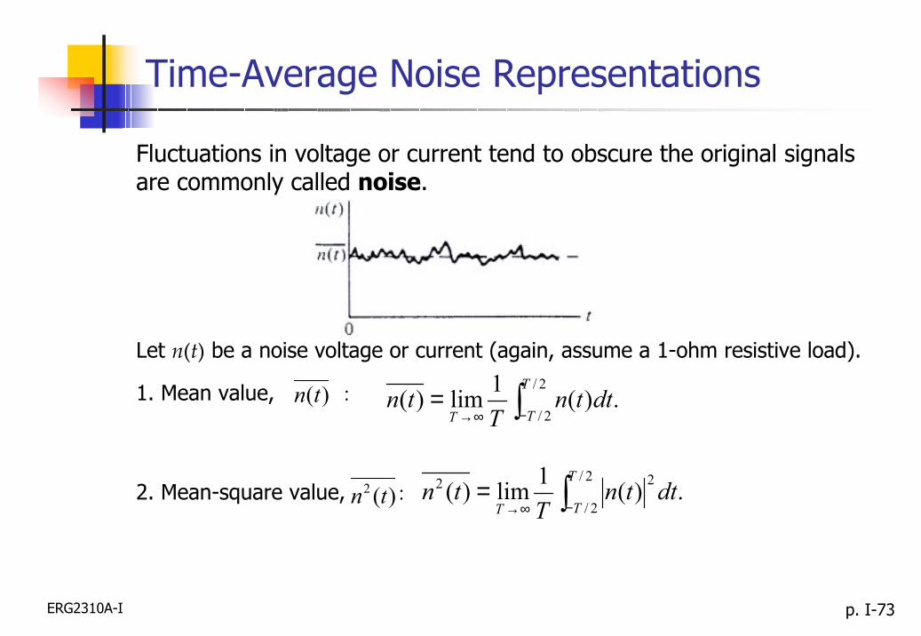
Time-Average Noise Representations
1. Mean value, :)(tn .)(1lim)(2/
2/∫−∞→=
T
TTdttn
Ttn
2. Mean-square value, :)(2 tn .)(1lim)(2/
2/
22 ∫−∞→=
T
TTdttn
Ttn
Fluctuations in voltage or current tend to obscure the original signals are commonly called noise.
Let n(t) be a noise voltage or current (again, assume a 1-ohm resistive load).
ERG2310A-I p. I-74
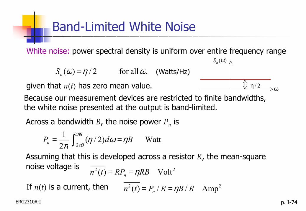
Band-Limited White Noise
White noise: power spectral density is uniform over entire frequency range
, allfor 2/)( ωηω =nS
given that n(t) has zero mean value. 2/η ω
)(ωnS
Because our measurement devices are restricted to finite bandwidths, the white noise presented at the output is band-limited.
Across a bandwidth B, the noise power Pn is
Watt)2/(21 2
2BdP
B
Bn ηωηπ
π
π== ∫−
Assuming that this is developed across a resistor R, the mean-square noise voltage is 22 Volt )( RBRPtn n η==
If n(t) is a current, then 22 Amp //)( RBRPtn n η==
(Watts/Hz)

ERG2310A-I p. I-75
Band-Limited White Noise
Suppose that the white noise ni(t) is transmitted through a linear time-invariant system with transfer function H(ω). The rms of output noise is given by
.)()(21
)(21)(
2
2
∫
∫∞
∞−
∞
∞−
ωωωπ
=
ωωπ
=
dHS
dStn
i
o
n
no
Since the power spectral density of the noise is white, we have
.)(2
)(22
1)(
0
2
22
∫
∫∞
∞
∞−
ωωπ
η=
ωωηπ
=
dH
dHtno

ERG2310A-I p. I-76
Equivalent Noise Bandwidth
The equivalent noise bandwidth BN is defined such that
(a) the power spectral density at the filter output is white within the bandwidth BN and zero elsewhere, forming an equivalent rectangular spectral density;
(b) the area under this rectangular spectral density is equal tothe area under the spectral density at the filter output.
ERG2310A-I p. I-77
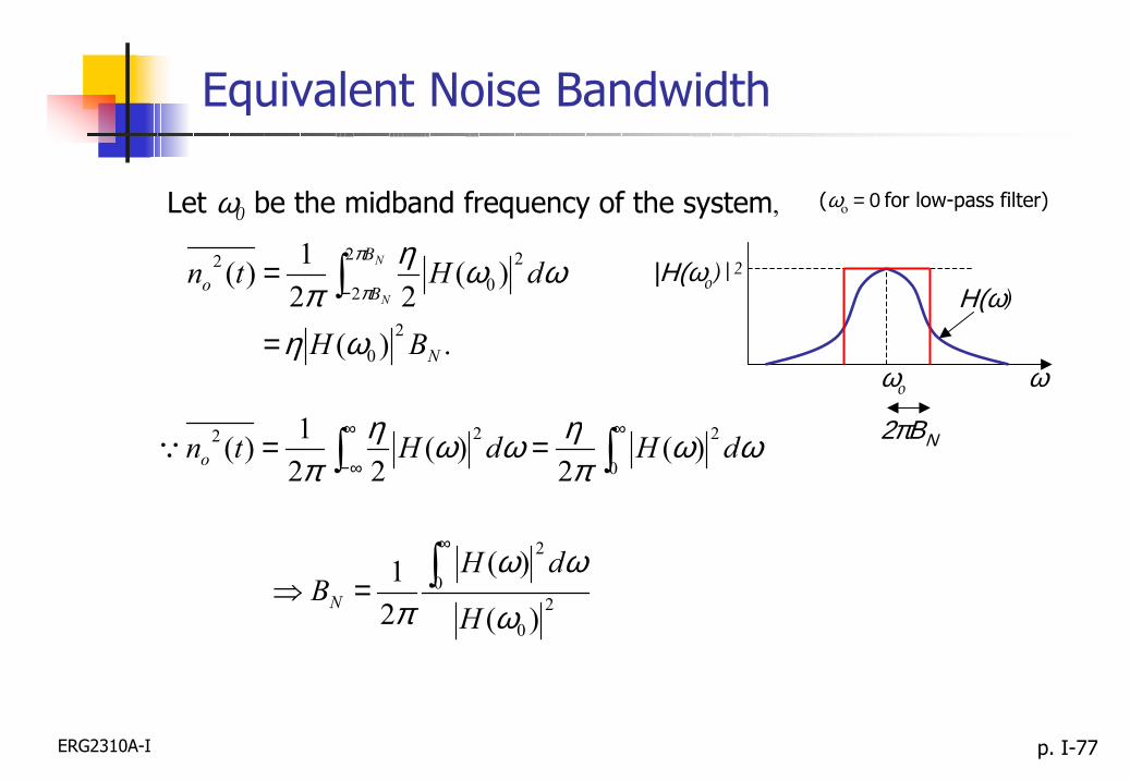
Equivalent Noise Bandwidth
Let ω0 be the midband frequency of the system,
.)(
)(22
1)(
20
2
2
20
2
N
B
Bo
BH
dHtn N
N
ωη
ωωηπ
π
π
=
= ∫−
20
0
2
)(
)(
21
ω
ωωπ H
dHBN
∫∞
=⇒
∫∫∞∞
∞−==
0
222 )(2
)(22
1)( ωωπηωωη
πdHdHtnoQ
ωo ω
|Η(ωo)|2
2πΒΝ
Η(ω)
(ωo = 0 for low-pass filter)
ERG2310A-I p. I-78
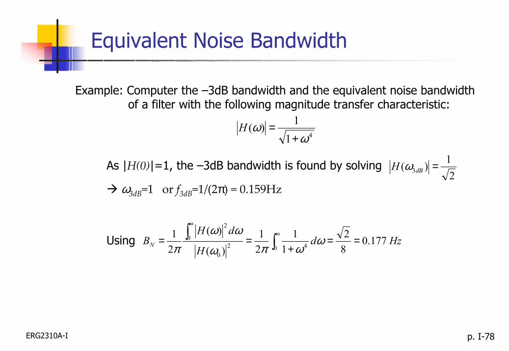
Equivalent Noise Bandwidth
Example: Computer the –3dB bandwidth and the equivalent noise bandwidth of a filter with the following magnitude transfer characteristic:
411)(ω
ω+
=H
As |H(0)|=1, the –3dB bandwidth is found by solving 2
1)( 3 =dBH ω
ω3dB=1 or f3dB=1/(2π) = 0.159Hz
∫∫ ∞
∞
==+
==0 42
0
0
2
177.082
11
21
)(
)(
21 Hzd
H
dHBN ω
ωπω
ωωπ
Using
ERG2310A-I p. I-79
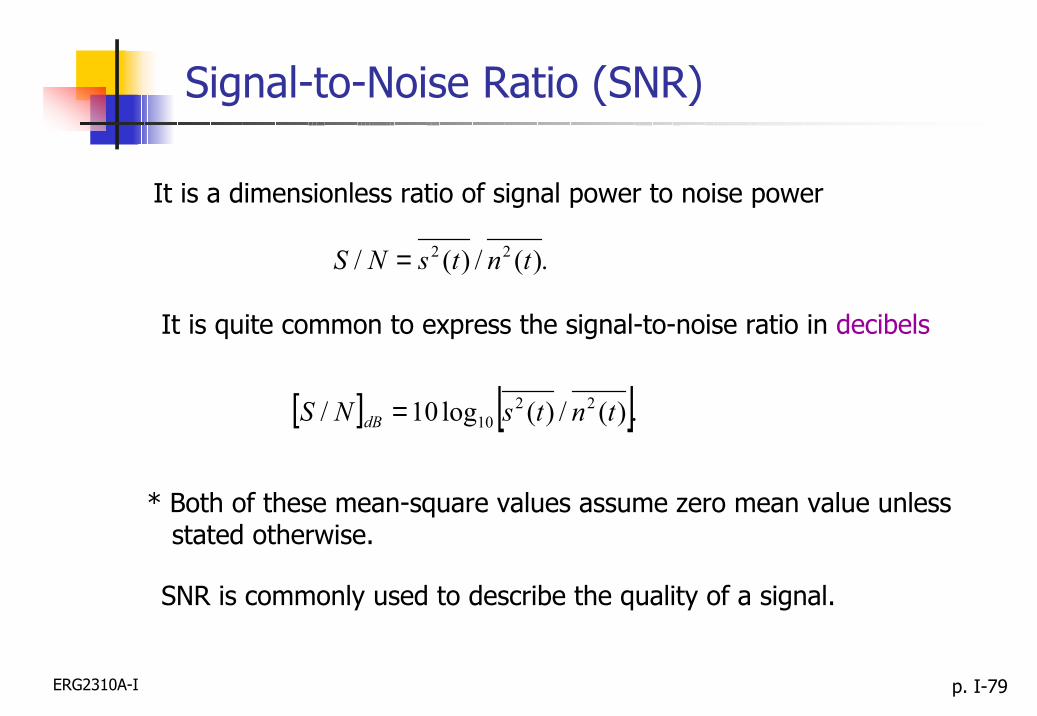
Signal-to-Noise Ratio (SNR)
It is a dimensionless ratio of signal power to noise power
.)(/)(/ 22 tntsNS =
It is quite common to express the signal-to-noise ratio in decibels
[ ] [ ].)(/)(log10/ 2210 tntsNS dB =
* Both of these mean-square values assume zero mean value unlessstated otherwise.
SNR is commonly used to describe the quality of a signal.
ERG2310A-I p. I-80
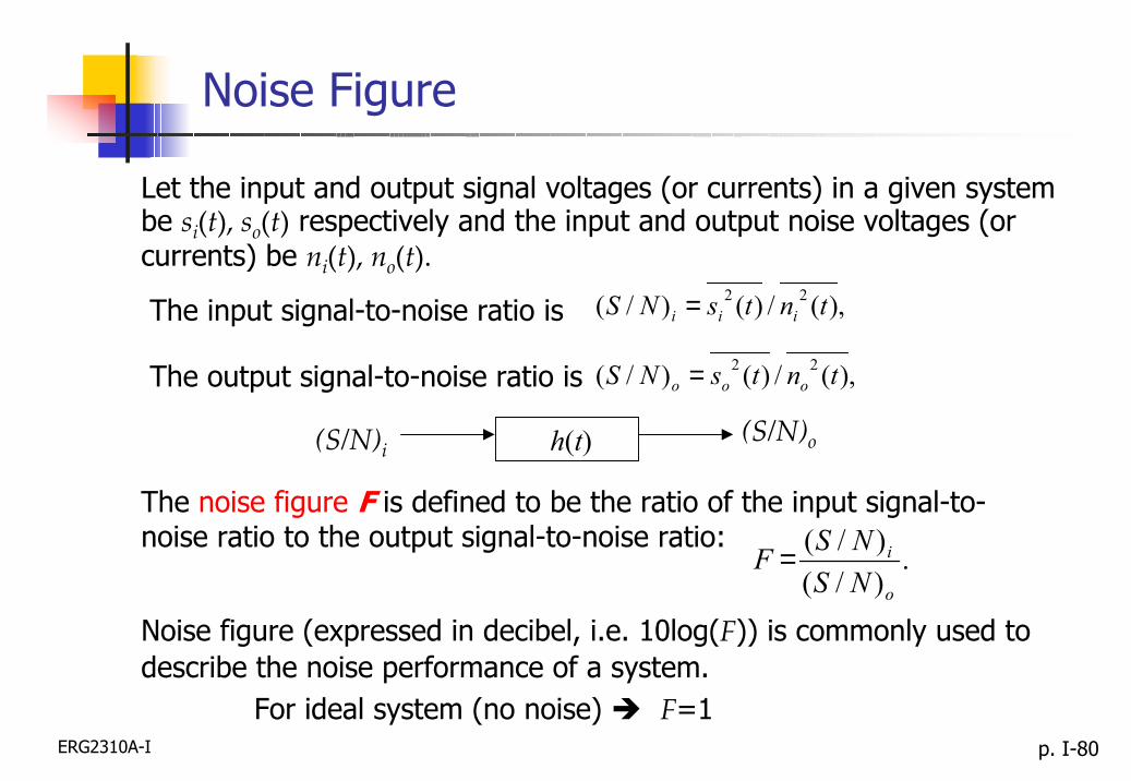
Noise Figure
Let the input and output signal voltages (or currents) in a given system be si(t), so(t) respectively and the input and output noise voltages (or currents) be ni(t), no(t).
The input signal-to-noise ratio is ,)(/)()/( 22 tntsNS iii =
The output signal-to-noise ratio is ,)(/)()/( 22 tntsNS ooo =
The noise figure F is defined to be the ratio of the input signal-to-noise ratio to the output signal-to-noise ratio:
.)/()/(
o
i
NSNSF =
(S/N)oh(t)(S/N)i
Noise figure (expressed in decibel, i.e. 10log(F)) is commonly used to describe the noise performance of a system.
For ideal system (no noise) F=1