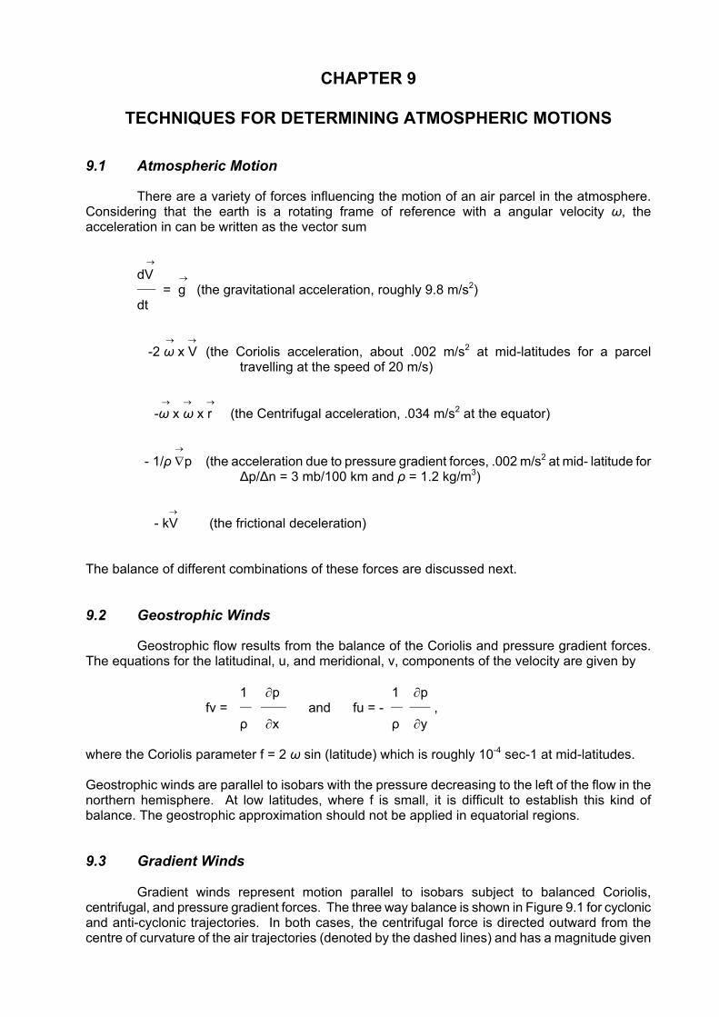
CHAPTER 9 TECHNIQUES FOR DETERMINING ATMOSPHERIC MOTIONS 9.1 Atmospheric Motion

There are a variety of forces influencing the motion of an air parcel in the atmosphere. Considering that the earth is a rotating frame of reference with a angular velocity ω, the acceleration in can be written as the vector sum

→

dV → = g (the gravitational acceleration, roughly 9.8 m/s2) dt

→ →

-2 ω x V (the Coriolis acceleration, about .002 m/s2 at mid-latitudes for a parcel travelling at the speed of 20 m/s)

→ → → -ω x ω x r (the Centrifugal acceleration, .034 m/s2 at the equator)

→

- 1/ρ ∇p (the acceleration due to pressure gradient forces, .002 m/s2 at mid- latitude for ∆p/∆n = 3 mb/100 km and ρ = 1.2 kg/m3)

→ - kV (the frictional deceleration)

The balance of different combinations of these forces are discussed next. 9.2 Geostrophic Winds

Geostrophic flow results from the balance of the Coriolis and pressure gradient forces. The equations for the latitudinal, u, and meridional, v, components of the velocity are given by

1 ∂p 1 ∂p fv = and fu = - ,

ρ ∂x ρ ∂y where the Coriolis parameter f = 2 ω sin (latitude) which is roughly 10-4 sec-1 at mid-latitudes. Geostrophic winds are parallel to isobars with the pressure decreasing to the left of the flow in the northern hemisphere. At low latitudes, where f is small, it is difficult to establish this kind of balance. The geostrophic approximation should not be applied in equatorial regions. 9.3 Gradient Winds

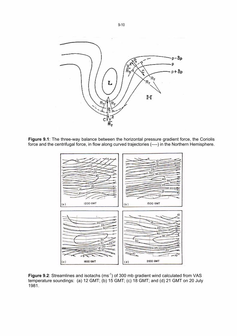
Gradient winds represent motion parallel to isobars subject to balanced Coriolis, centrifugal, and pressure gradient forces. The three way balance is shown in Figure 9.1 for cyclonic and anti-cyclonic trajectories. In both cases, the centrifugal force is directed outward from the centre of curvature of the air trajectories (denoted by the dashed lines) and has a magnitude given

9-2

by V2/RT, where RT is the local radius of curvature. In effect, a balance of forces can be achieved with a wind velocity smaller than would be required if the Coriolis force were acting alone. Thus, in this case, it is possible to maintain a sub-geostrophic flow parallel to the isobars. For the anti-cyclonically curved trajectory, the situation is just the opposite: the centrifugal force opposes the Coriolis force and, in effect, necessitates a super-geostrophic wind velocity in order to bring about a three-way balance of forces.

If Pn denotes the normal component of the pressure gradient force per unit mass and f the Coriolis parameter, we can write

V2 pn = fV ±

RT

The geopotential height fields derived from the TIROS or VAS data can be used to evaluate the gradient wind. This is accomplished by realizing

1 ∂p ∂Z Pn = - = - go

ρ ∂n ∂n

and then solving for V by using the quadratic formula.

Figure 9.2 shows streamlines and isotachs of 300 mb gradient winds derived from VAS temperature profile data, where the curvature term is approximated from the geopotential height field contours. As can be seen, the depiction of the flow is quite detailed with a moderately intense subtropical jet streak propagating east-southeastward in time. Such wind fields in time sequence are especially useful in nowcasting applications.

Gradient winds have also been compared on a routine basis with conventional radiosonde and dropwindsonde determinations by NHC as part of the NOVA programme. During 1982, the VAS gradient winds averaged about 30% shower than the conventionally observed winds. Several factors may be contributing to this discrepancy: ageostrophic motions, deficient height fields in data void areas, and inaccurate determination of the normal derivation of the geopotential height due to the resolution of the analysis field. Most likely, the last factor is very significant. Whatever the cause, for 1982 NHC concluded that gradient winds were less useful than cloud motion winds in their analyses. 9.4 Thermal Winds

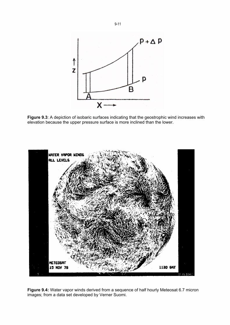
Thermal winds give a measure of the vertical wind shear. This can be seen qualitatively by considering two surfaces of constant pressure in a vertical cross section, as in Figure 9.3. Since the geostrophic wind is proportional to the slopes of the isobaric surfaces, the geostrophic wind increases with elevation because the upper pressure surface is more inclined than the lower. The increased slope for the higher surface is revealed in the finite-difference form of the hydrostatic equation:

∆p ∆z ≈ -

ρg The pressure difference between the two surfaces is the same for columns A and B, so the difference in separation between them is due to a decrease in density in going from A to B. The average pressure is the same in the two columns, so column B has a higher average temperature

9-3

than column A. In this way we see that the geostrophic wind with elevation must be associated with a quasi-horizontal temperature gradient.

As this previous discussion indicates, the temperature gradient is measured along an isobaric surface, not along a horizontal surface. Thus, the vertical wind shear can be related to the horizontal gradient of temperature plus a correction term involving the slope of the isobaric surface and the temperature variation in the vertical. However, since the slopes of isobaric surfaces are generally quite small (of the order of 1/5000), the correction term is usually quite small also.

Quantitatively, the thermal wind relation is derived from the geostrophic wind equations,

1 ∂p 1 ∂p fv = and fu = - ,

ρ ∂x ρ ∂y together with the hydrostatic equation and the equation of state,

1 ∂p p g = - and ρ = .

ρ ∂z RT Note that there are five dependent variables, u, v, ρ, p, T and only four equations. A complete solution is not possible, but a useful interrelationship is readily available if ρ is eliminated in the geostrophic and hydrostatic expressions by means of the equation of state. This yields:

fv ∂ ln p fu ∂ ln p g ∂ ln p = R ; = - R ; = - T ∂x T ∂y T ∂z

After cross differentiating, the results are:

∂ fv ∂ g ∂ fu ∂ g ( ) = - ( ); ( ) ( ) = ( ) . ∂z T ∂x T ∂z T ∂y T

Rearranging, we get the thermal wind equations in differential form

∂v g ∂T v ∂T = + ∂z fT ∂x T ∂z

∂u g ∂T u ∂T = - + ∂z fT ∂y T ∂z

They have the characteristics which were physically anticipated since the first terms on the right are the contribution of the horizontal temperature gradient, and the second terms on the right are correction terms involving the slopes of the isobaric surface (u, v) and the vertical temperature gradients. The correction terms on the right are indeed relatively small. For the fractional rate of change of u with height, the correction term is (1/T)(∂T/∂z). Even if the lapse rate is as high as the dry adiabatic, this is about four percent per kilometre. The normal shear of west wind with height in the troposphere in middle latitudes is approximately 25 percent per kilometre. Thus, it is apparent that the additional term in question does not usually make a major contribution to the vertical wind shear, although there are situations were it must be taken into account.

9-4

Thus in the simpler form we write

∂v g ∂T ∂u g ∂T ≈ ; ≈ - ∂z fT ∂x ∂z fT ∂y

These equations require that for v to increase with height temperature must increase to the east, and for u to increase with height temperature must increase to the south, in the Northern Hemisphere. The fact that actual westerly winds in middle latitudes normally increase in strength going upward through the troposphere is to be explained, therefore, as a result of the normal decrease of temperature towards the poles in the troposphere.

By taking the difference at two levels (denoted here by a lower level 1 and upper level 2), one finds

go ∂T v2 - v1 = ( z2 - z1 ) .

fT ∂x Or one can substitute for the geopotential height to write

p1 R ∂T v2 - v1 = ln( ) .

p2 f ∂x A similar expression for the u component of the wind is readily derived.

Through the use of the thermal wind equation, it is possible to define a wind field from geopotential height observations at two reference levels and temperature profiles over the area of interest. Thus, a set of sea level pressure observations together with a grid of TIROS or VAS infrared temperature soundings constitutes a sufficient observing system for determining the three dimensional distribution of the thermal wind velocities. 9.5 Inferring Winds From Cloud Tracking

Geostationary satellite imagery has been used as a source of wind observations since the launch of the first spin scan camera aboard the Application Technology Satellite (ATS 1) in December 1966. It was recognized immediately that features tracked in a time sequence of images could provide estimates of atmospheric motion. Historically, wind vectors have been produced from images of visible (for low level vectors) and infrared longwave window radiation (for upper and low level vectors and some mid level vectors). In order to improve the coverage at mid levels and over cloud free areas, wind tracking has been applied to water vapour imagery at 6.7 and 7.2 microns (see Figure 9.4 for an example from Meteosat). Recently polar winds have been inferred from sequences of polar orbiting MODIS images in the arctic and Antarctic.

The basic elements of wind vector production have not changed since their inception. These are: (a) selecting a feature to track or a candidate target; (b) tracking the target in a time sequence of images to obtain a relative motion; (c) assigning a pressure height (altitude) to the vector; and (d) assessing the quality of the vector. Initially, these elements were done manually (even to the point of registering the images into a movie loop), but the goal has always been to automate procedures and reduce the time consuming human interaction.

To use a satellite image, the feature of interest must be located accurately on the earth. Since the earth moves around within the image plane of the satellite because of orbit effects, satellite orbit and attitude (where the satellite is and how it is oriented in space) must be determined and accounted for. This process of navigation is crucial for reliable wind vector determination. With

9-5 the assistance of landmarks (stars) to determine the attitude (orbit) of the spacecraft over time, earth location accuracies within one visible pixel (one km) have been realized.

The basic concept behind the cloud drift winds is that some clouds are passive tracers of

the atmosphere's motion in the vicinity of the cloud. However, clouds grow and decay with lifetimes which are related to their size. To qualify for tracking, the tracer cloud must have a lifetime that is long with respect to the time interval of the tracking sequence. The cloud must also be large compared with the resolution of the images. This implies a match between the spatial and temporal resolution of the image sequence. In order for a cloud to be an identifiable feature on an image, it generally must occupy an area at least ten to 20 pixels across (where pixel denotes a field of view). Hence for full resolution 1.0 km GOES visible data, the smallest clouds which can be used for tracking are 10 to 20 km across. Experience has shown that a time interval of approximately 3 to 10 min between images is necessary to track clouds of this size, with the shorter time interval being required for disturbed situations. For 4 km infrared images, the cloud tracers are about 100 km across, are tracked at half hour intervals, and represent an average synoptic scale flow. Water vapour images are found to hold features longer and are best tracked at hourly intervals (a longer time interval offers better accuracy of the tracer if the feature is not changing).

Cloud drift winds compare within 5 to 8 m/s with radiosonde wind observations. However, it must be recognized that cloud winds represent a limited and meteorologically biased data set. The cloud winds generally yield measurements from only one level (the uppermost layer of the cloud) and from regions where the air is going up (and producing clouds). Even with the water vapour motions enhancing the cloud drift winds, the meteorological bias persists. Satellite derived winds are best used over data sparse regions to fill in some of the data gaps between radiosonde stations and between radiosonde launch times. 9.5.1 Current Operational Procedures

Operational winds from GOES are derived from a sequence of three navigated and earth located images taken 30 minutes apart. Cloud Motion Vectors (CMVs) are calculated by a three-step objective procedure. The initial step selects targets, the second step assigns pressure altitude, and the third step derives motion. Altitude is assigned based on a temperature/pressure derived from radiative transfer calculations in the environment of the target. Motion is derived by a pattern recognition algorithm that matches a feature within the "target area" in one image within a "search area" in the second image. For each target two winds are produced representing the motion from the first to the second, and from the second to the third image. An objective editing scheme is then employed to perform quality control: the first guess motion, the consistency of the two winds, the precision of the cloud height assignment, and the vector fit to an analysis are all used to assign a quality flag to the "vector" (which is actually the average of the two vectors).

Water Vapor Motion Vectors (WVMVs) are inferred from the imager band at 6.7 microns

which sees the upper troposphere and sounder bands at 7.0 and 7.5 microns which see deeper into the troposphere. WVMVs are derived by the same methods used with CMVs. Heights are assigned from the water vapor brightness temperature in clear sky conditions and from radiative transfer techniques in cloudy regions.

In 1998, the National Environmental Satellite, Data, and Information Service (NESDIS)

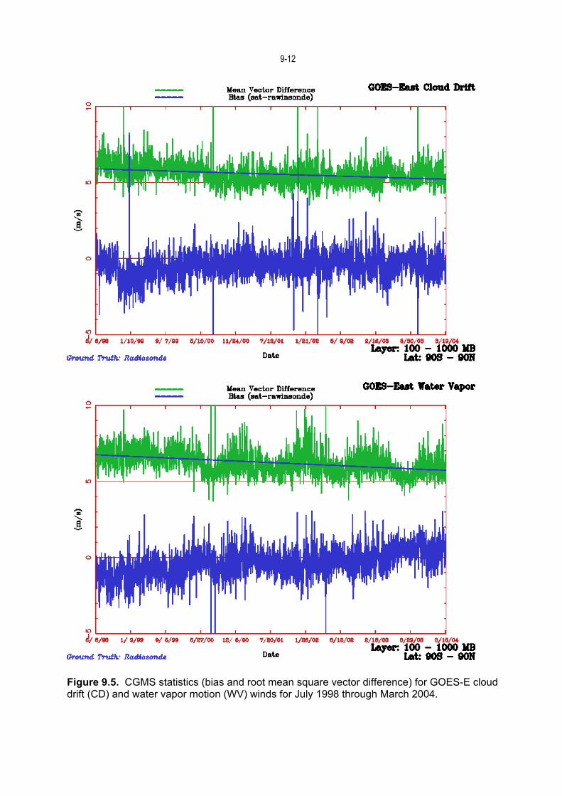
operational GOES-8/9/10 CMV and WVMV production increased to every three hours with high spatial density tracers derived from visible, infrared window, and water vapor images. The number of motion vectors has increased dramatically to over 10 000 vectors for each winds data set. The quality of the wind product is being reported monthly in accordance with the Coordination Group for Meteorological Satellites (CGMS) reporting procedures (Schmetz et al., 1997 and 1999); this involves direct comparisons of collocated computed cloud motions and radiosonde observations. It reveals GOES cloud motion wind RMS differences to be within 6.5 to 7 m/s with respect to raobs, with a slow bias of about .5 m/s; water vapor motions RMS differences are within 7 to 7.5 m/s (Nieman et al., 1997). The NESDIS operational winds inferred from infrared window and water vapor images continue to perform well. Figure 9.5 presents the summary from 1998 through 2004.

9-6 The next few paragraphs describe the current operational procedures.

(a) Tracer Selection

In the 1990s, tracer selection for GOES winds was improved. In the old tracer selection algorithm, the highest pixel brightness values within each target domain were found, local gradients were computed around those locations, and adequately large gradients were assigned as target locations. In the new tracer selection algorithm, maximum gradients are subjected to a spatial-coherence analysis. Too much coherence indicates such features as coastlines and thus is undesirable. The presence of more than two coherent scenes often indicates mixed level clouds; such cases are screened. The resulting vectors from the new scheme (Figure 9.6) show a much higher density of tracers in desirable locations. (b) Height Assignment Techniques

Semi-transparent or sub-pixel clouds are often the best tracers, because they show good

radiance gradients that can readily be tracked and they are likely to be passive tracers of the flow at a single level. Unfortunately their height assignments are especially difficult. Since the emissivity of the cloud is less than unity by an unknown and variable amount, its brightness temperature in the infrared window is an overestimate of its actual temperature. Thus, heights for thin clouds inferred directly from the observed brightness temperature and an available temperature profile are consistently low.

Presently heights are assigned by any of three techniques when the appropriate spectral

radiance measurements are available (Nieman et al., 1993). In opaque clouds, infrared window (IRW) brightness temperatures are compared to forecast temperature profiles to infer the level of best agreement which is taken to be the level of the cloud. In semi-transparent clouds or sub-pixel clouds, since the observed radiance contains contributions from below the cloud, this IRW technique assigns the cloud to too low a level. Corrections for the semi-transparency of the cloud are possible with the carbon dioxide (CO2) slicing technique (Menzel et al., 1983) where radiances from different layers of the atmosphere are ratioed to infer the correct height. A similar concept is used in the water vapor (H2O) intercept technique (Szejwach, 1982), where the fact that radiances influenced by upper tropospheric moisture (H2O) and IRW radiances exhibit a linear relationship as a function of cloud amount is used to extrapolate the correct height.

An IRW estimate of the cloud height is made by averaging the infrared window brightness

temperatures of the coldest 25 percent of pixels and interpolating to a pressure from a forecast guess sounding (Merrill et al. 1991).

In the CO2 slicing technique, a cloud height is assigned with the ratio of the deviations in

observed radiances (which include clouds) from the corresponding clear air radiances for the infrared window and the CO2 (13.3 micron) channel. The clear and cloudy radiance differences are determined from observations with GOES and radiative transfer calculations. Assuming the emissivities of the two channels are roughly the same, the ratio of the clear and cloudy radiance differences yields an expression by which the cloud top pressure of the cloud within the FOV can be specified. The observed differences are compared to a series of radiative transfer calculations with possible cloud pressures, and the tracer is assigned the pressure that best satisfies the observations. The operational implementation is described in Merrill et al. (1991).

The H2O intercept height assignment is predicated on the fact that the radiances for two

spectral bands vary linearly with cloud amount. Thus a plot of H2O (6.5 micron) radiances versus IRW (11.0 micron) radiances in a field of varying cloud amount will be nearly linear. These data are used in conjunction with forward calculations of radiance for both spectral channels for opaque clouds at different levels in a given atmosphere specified by a numerical weather prediction of temperature and humidity. The intersection of measured and calculated radiances will occur at

9-7 clear sky radiances and cloud radiances. The cloud top temperature is extracted from the cloud radiance intersection (Schmetz et al., 1993).

Satellite stereo height estimation has been used to validate H2O intercept height

assignments. The technique is based upon finding the same cloud patch in several images. For cloud motion, the cloud needs to change slowly relative to the image frequency. For stereo heights, the cloud needs to be distinct and appear nearly the same from the two viewpoints (after re-mapping to the same projection). Campbell (1998) built upon earlier work of Fujita and others (Fujita, 1982) to develop a method which adjusts for the motion of the cloud so that simultaneity is not required for the stereo height estimate. A test analysis was performed with Meteosat – 5 / 7 data; stereo heights and H2O intercept heights agreed within 50 hPa. As more geostationary and polar orbiting satellites remain in operation, the prospects for geometric stereo height validations of the operational IRW, H2O intercept, and CO2 slicing heights become very promising. (c) Objective Editing

Automated procedures for deriving cloud-motion vectors from a series of geostationary

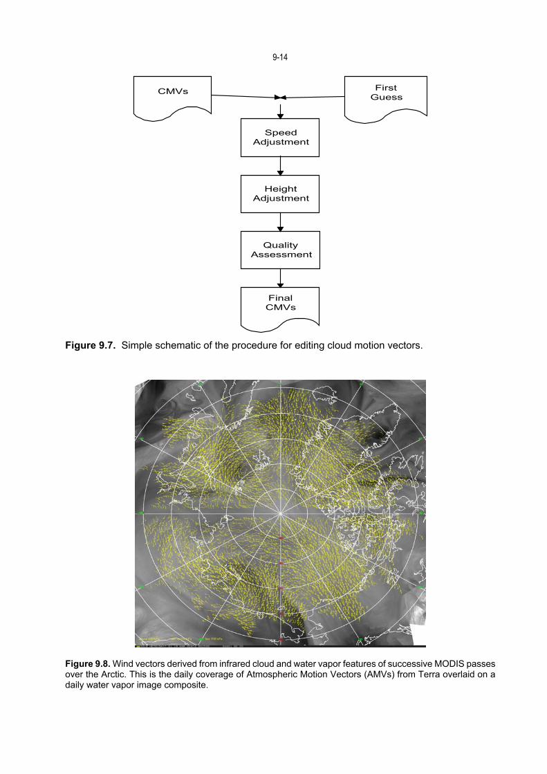
infrared-window images first became operational in the National Oceanic and Atmospheric Administration (NOAA) in 1993 (Merrill et al., 1991). NESDIS has been producing GOES-8 / 9 / 10 cloud motion vectors without manual intervention. Suitable tracers are automatically selected within the first of a sequence of images (see section 2a) and heights are assigned using the H2O intercept method. Tracking features through the subsequent imagery is automated using a covariance minimization technique (Merrill et al., 1991) and an automated quality-control algorithm (Hayden and Nieman, 1996) is applied. Editing the CMVs through analyses with respect to a first guess wind and temperature profile field involves speed adjustment, height adjustment, and quality assessment (Figure 9.7). This procedure, with some modifications, is also used to infer water vapor motion vectors; tracer selection is based on gradients within the target area and vector heights are inferred from the water vapor brightness temperatures.

To mitigate the slow bias found in upper-level GOES CMV in extra-tropical regions, each

vector above 300 hPa is incremented by 8 percent of the vector speed. There are indications that the slow bias can be attributed to (a) tracking winds from sequences of images separated by too much time, (b) estimating atmospheric motion vectors from inappropriate tracers, and (c) height assignment difficulties. Some also suggest that cloud motions will not indicate full atmospheric motions in most situations.

A height adjustment is accomplished through a first-pass analysis of the satellite-derived

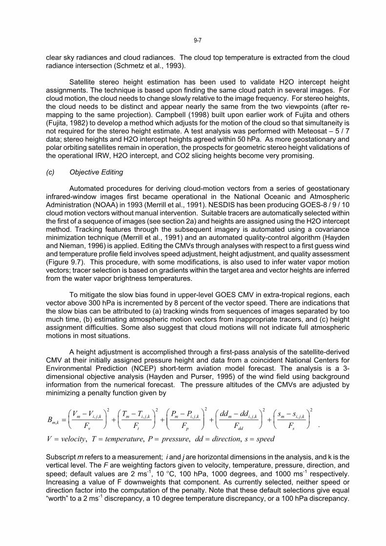
CMV at their initially assigned pressure height and data from a coincident National Centers for Environmental Prediction (NCEP) short-term aviation model forecast. The analysis is a 3-dimensional objective analysis (Hayden and Purser, 1995) of the wind field using background information from the numerical forecast. The pressure altitudes of the CMVs are adjusted by minimizing a penalty function given by

BV VF

T TF

P PF

dd ddF

s sF

V velocity T temperature P pressure dd direction s speed

m km i j k

v

m i j k

t

m i j k

p

m i j k

dd

m i j k

s,

, , , , , , , , , ,

, , , ,

=−

+

−

+

−

+

−

+

−

= = = = =

2 2 2 2 2

.

Subscript m refers to a measurement; i and j are horizontal dimensions in the analysis, and k is the vertical level. The F are weighting factors given to velocity, temperature, pressure, direction, and speed; default values are 2 ms-1, 10 οC, 100 hPa, 1000 degrees, and 1000 ms-1 respectively. Increasing a value of F downweights that component. As currently selected, neither speed or direction factor into the computation of the penalty. Note that these default selections give equal “worth” to a 2 ms-1 discrepancy, a 10 degree temperature discrepancy, or a 100 hPa discrepancy.

9-8 Further details can be found in Velden et al. (1998).

The pressure levels for height adjustment in hPa are 925, 850, 775, 700, 600, 500, 400, 350, 300, 250, 200, 150, and 100. The pressure or height reassignment is constrained to 100 hPa. A tropopause test looks for lapse rates of less than 0.5 K per 25 hPa above 300 hPa and prohibits re-assignment to stratospheric heights. (d) Quality Flags

A quality assessment for each vector is accomplished by a second analysis using the CMVs

at the reassigned pressure altitudes and by inspecting the local quality of the analysis and the fit of the observation to that analysis. Thresholds are given for rejecting the data. Accepted data and the associated quality estimate, denoted by RFF for Recursive Filter Flag, are passed to the user (Hayden and Purser, 1995).

Several options are available for regulating the analysis, the penalty function, and the final

quality estimates. These have been optimized, over several years of application, for the operational GOES CMVs. However the optimization may be situation dependent; what works best with GOES CMVs may not be optimal for WVMVs or winds generated at higher density, or winds generated with an improved background forecast, etc. Research on optimal tuning of this system in its various applications continues (Velden et al., 1998).

The EUropean organization for the exploitation for METeorological SATellites (EUMETSAT)

has developed a quality indicator (QI) for use with Meteosat data that checks for direction, speed, and vector consistency in the vector pairs (derived from the three images in the wind determining sequence). In addition, consistency with nearest neighbors vectors and with respect to a forecast model are factored in. A weighted average of these five consistency checks becomes the QI.

Depending on the synoptic situation between 10 and 33% of the processed tracers are

rejected in the cloud vector inspection and quality flag assignment. A combination of the EUMETSAT QI and the NESDIS RFF wind quality indicators has been shown to enhance utilization of the high-density CMVs in numerical weather prediction models and is in the process of being implemented (Holmlund et al., 1999). (e) Recent Upgrades

The major operational changes in the past years are summarized as follows. (1) Winds

inferred from visible image loops as well as sounder mid-level moisture sensitive bands were added to operations by summer 1998. (2) This enabled ensemble auto-editing, where the combined wind sets from visible, infrared window, three water vapor sensitive bands are compared for consistency. The dependency on a numerical weather prediction (NWP) model first guess was diminished. (3) A dual pass auto-editor was put in place by summer 1998 that relaxes rejection criteria for winds around a feature of interest and use normal procedures elsewhere. This enables better retention of the tighter circulation features associated with tropical cyclones and other severe weather. (4) Water vapor winds were designated as being determined in clear skies or over clouds; the clear sky WVMVs are representative of layer mean motion while cloudy sky WVMVs are cloud top motion. (5) A quality flag that combines QI and RFF has been attached to each wind vector indicating the level of confidence resulting from the post-processing. 9.5.2 Polar Winds

The feasibility of deriving tropospheric wind information at high latitudes from the MODIS instrument aborad the Terra and Aqua satellites has been demonstrated by CIMSS (Santek et al, 2002; Key et al, 2003). Cloud and water vapor tracking with MODIS data is based on the established procedures used for GOES, which are essentially those described in Nieman et al.

9-9 (1997) and Velden et al. (1997, 1998). With MODIS, cloud features are tracked in the IR window band at 11 µm and water vapor (WV) features are tracked using the 6.7 µm band. An example of typical MODIS AMV coverage is shown in Figure 9.8. Additional details are given in Key et al., 2004

Orbital characteristics, low water vapor amounts, a relatively high frequency of thin, low clouds, and complex surface features create some unique challenges for the retrieval of high-latitude AMV. Nevertheless, initial model impact studies with the MODIS polar AMVs conducted at the European Center for Medium Range Weather Forecasting (Bormann and Thepaut, 2004) and the NASA Global Modeling and Assimilation Office (GMAO) were encouraging enough, such that these winds are now being assimilated on an operational basis at ECMWF.

References Bormann, N, and J.-N. Thepaut, 2004: Impact of MODIS Polar Winds in ECMWF’s 4DVAR Data Assimilation System, Monthly Wea. Rev. 132, 929-940. Key, J., D. Santek, C.S. Velden, N. Bormann, J.-N. Thepaut, L.P. Riishojgaard, Y. Zhu, and W.P. Menzel, 2003, Cloud-drift and Water Vapor Winds in the Polar Regions from MODIS, IEEE Trans. Geosci. Remote Sensing, 41(2), 482-492. Santek, D., J. Key, C. Velden, and N. Borman, 2002: Deriving winds from polar orbiting satellite data. Proc. Sixth Int. Winds Workshop, Madison, Wisconsin, EUMETSAT, 251-261.

9-10

Figure 9.1: The three-way balance between the horizontal pressure gradient force, the Coriolis force and the centrifugal force, in flow along curved trajectories (----) in the Northern Hemisphere.

Figure 9.2: Streamlines and isotachs (ms-1) of 300 mb gradient wind calculated from VAS temperature soundings: (a) 12 GMT; (b) 15 GMT; (c) 18 GMT; and (d) 21 GMT on 20 July 1981.

9-11

Figure 9.3: A depiction of isobaric surfaces indicating that the geostrophic wind increases with elevation because the upper pressure surface is more inclined than the lower.

Figure 9.4: Water vapor winds derived from a sequence of half hourly Meteosat 6.7 micron images; from a data set developed by Verner Suomi.

9-12

Figure 9.5. CGMS statistics (bias and root mean square vector difference) for GOES-E cloud drift (CD) and water vapor motion (WV) winds for July 1998 through March 2004.

9-13

Figure 9.6. Vector distribution resulting from the pre-GOES-8 (top) and post-GOES-8 (bottom) tracer selection capabilities. Wind vectors shown represent the improvements in the vector density realized in this decade. The images are from 25 August 1998 during Hurricane Bonnie. Heights of the wind vectors (see section 2b) are indicated by color; yellow between 150 and 250 hPa, orange between 251 and 350 hPa, and white between 351 and 600 hPa.

9-14

CMVs FirstGuess

FinalCMVs

SpeedAdjustment

HeightAdjustment

QualityAssessment

Figure 9.7. Simple schematic of the procedure for editing cloud motion vectors.

Figure 9.8. Wind vectors derived from infrared cloud and water vapor features of successive MODIS passes over the Arctic. This is the daily coverage of Atmospheric Motion Vectors (AMVs) from Terra overlaid on a daily water vapor image composite.