Chapter 9 Lecture: The Schwarzschild...
40
Chapter 9 Lecture: The Schwarzschild Spacetime One of the simplest solutions to the Einstein equations corresponds to a metric that describes the gravitational field exterior to a static, spherical, uncharged mass with- out angular momentum and isolated from all other mass (Schwarzschild, 1916). The Schwarzschild solution is • A solution to the vacuum Einstein equations G μν = R μν = 0. • Only valid in the absence of matter and non-gravitational fields (T μν = 0). • Spherically symmetric and time independent. 193
Transcript of Chapter 9 Lecture: The Schwarzschild...
Chapter 9
Lecture: The SchwarzschildSpacetime
One of the simplest solutions to the Einstein equationscorresponds to a metric that describes the gravitationalfield exterior to a static, spherical, uncharged mass with-out angular momentum and isolated from all other mass(Schwarzschild, 1916).
The Schwarzschild solution is
• A solution to the vacuum Einstein equationsGµν = Rµν = 0.
• Only valid in the absence of matter and non-gravitational fields(Tµν = 0).
• Spherically symmetric and time independent.
193
194 CHAPTER 9. LECTURE: THE SCHWARZSCHILD SPACETIME
Thus, the Schwarzschild solution is valid outside spher-ical mass distributions, but the interior of a star will bedescribed by a different metric that must be matched atthe surface to the Schwarzschild one.
9.1. THE FORM OF THE METRIC 195
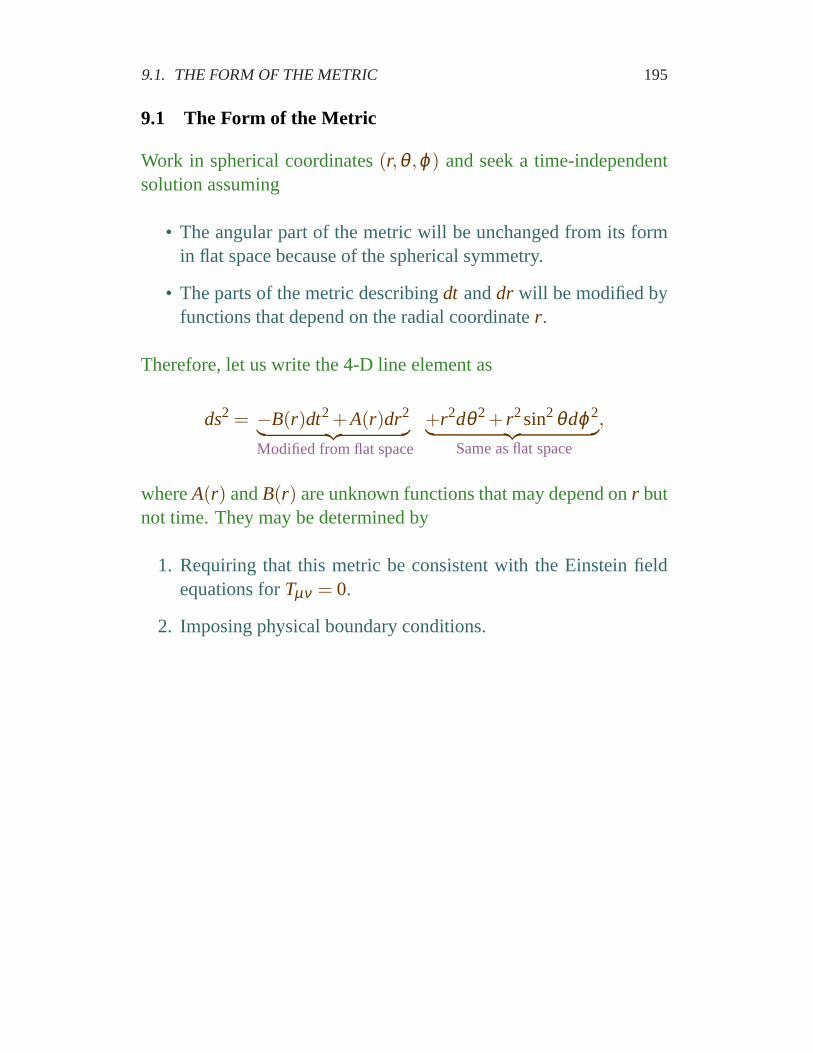
9.1 The Form of the Metric
Work in spherical coordinates(r,θ ,ϕ) and seek a time-independentsolution assuming
• The angular part of the metric will be unchanged from its formin flat space because of the spherical symmetry.
• The parts of the metric describingdt anddr will be modified byfunctions that depend on the radial coordinater .
Therefore, let us write the 4-D line element as
ds2 = −B(r)dt2 +A(r)dr2︸ ︷︷ ︸
Modified from flat space
+r2dθ2+ r2sin2θdϕ2︸ ︷︷ ︸
Same as flat space
,
whereA(r) andB(r) are unknown functions that may depend onr butnot time. They may be determined by
1. Requiring that this metric be consistent with the Einstein fieldequations forTµν = 0.
2. Imposing physical boundary conditions.
196 CHAPTER 9. LECTURE: THE SCHWARZSCHILD SPACETIME
Boundary conditions:Far from the star gravity becomesweak so
Limr→∞
A(r) = Limr→∞
B(r) = 1.
Substitute the metric form in vacuum Einstein and impose these bound-ary conditions (Exercise):
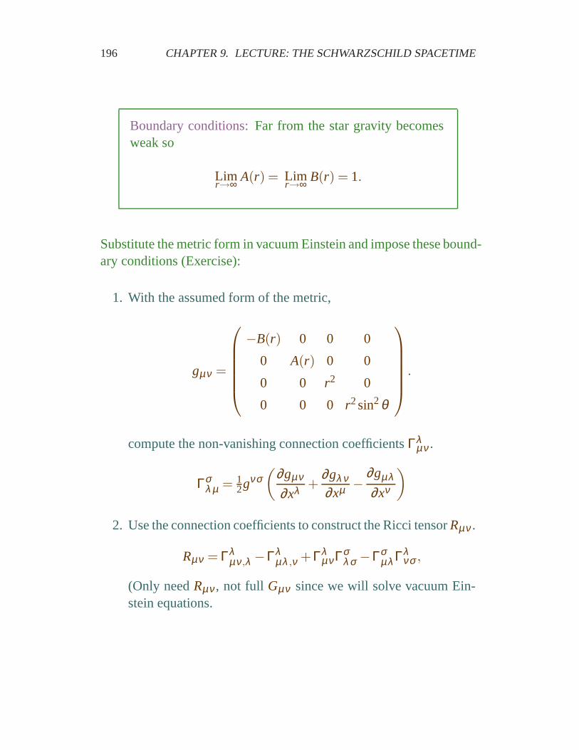
1. With the assumed form of the metric,
gµν =
−B(r) 0 0 0
0 A(r) 0 0
0 0 r2 0
0 0 0 r2sin2θ
.
compute the non-vanishing connection coefficientsΓλµν .
Γσλ µ = 1
2gνσ(
∂gµν
∂xλ +∂gλν∂xµ −
∂gµλ∂xν
)
2. Use the connection coefficients to construct the Ricci tensorRµν .
Rµν = Γλµν ,λ −Γλ
µλ ,ν +ΓλµνΓσ
λσ −Γσµλ Γλ
νσ ,
(Only needRµν , not full Gµν since we will solve vacuum Ein-stein equations.
9.1. THE FORM OF THE METRIC 197
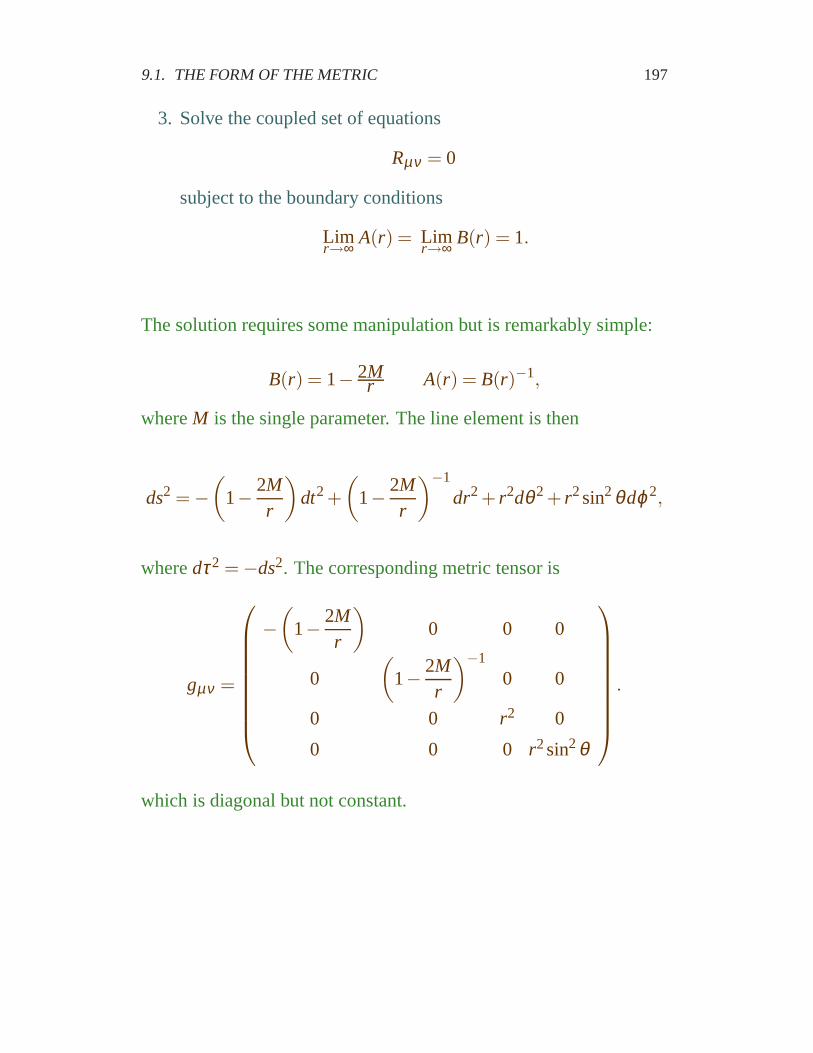
3. Solve the coupled set of equations
Rµν = 0
subject to the boundary conditions
Limr→∞
A(r) = Limr→∞
B(r) = 1.
The solution requires some manipulation but is remarkably simple:
B(r) = 1− 2Mr A(r) = B(r)−1,
whereM is the single parameter. The line element is then
ds2 =−(
1− 2Mr
)
dt2+
(
1− 2Mr
)−1
dr2+ r2dθ2+ r2sin2θdϕ2,
wheredτ2 =−ds2. The corresponding metric tensor is
gµν =
−(
1− 2Mr
)
0 0 0
0
(
1− 2Mr
)−1
0 0
0 0 r2 0
0 0 0 r2sin2θ
.
which is diagonal but not constant.
198 CHAPTER 9. LECTURE: THE SCHWARZSCHILD SPACETIME
By comparing
g00 =−(
1− 2GMrc2
)
︸ ︷︷ ︸
Weak gravity (earlier)
←→ g00 =−(
1− 2GMrc2
)
︸ ︷︷ ︸
Schwarzschild (G & c restored)
we see that the parameterM (mathematically the single free parameterof the solution) may be identified with thetotal mass that is the sourceof the gravitational curvature:
• Rest mass
• Contributions from mass–energy densities and pressure
• Energy from spacetime curvature
From the structure of the metric
ds2 =−B(r)dt2 +A(r)dr2+ r2dθ2+ r2sin2θdϕ2,
• θ andϕ have similar interpretations as for flat space.
• The coordinate radiusr generally cannot be interpreted as aphysical radius becauseA(r) 6= 1.
• Thecoordinate timet generally cannot be interpreted as a phys-ical clock time becauseB(r) 6= 1.
The quantityrS≡ 2M
is called theSchwarzschild radius.It plays a central rolein the description of the Schwarzschild spacetime.

9.1. THE FORM OF THE METRIC 199
r/Mgµν
r =
2M
g11
g11
g00
+
−
Figure 9.1:The componentsg00 andg11 in the Schwarzschild metric.
The line element (metric)
ds2 =−(
1− 2Mr
)
︸ ︷︷ ︸g00
dt2+
(
1− 2Mr
)−1
︸ ︷︷ ︸g11
dr2+ r2dθ2+ r2sin2θdϕ2
appears to contain two singularities (see above figure)
1. A singularity atr = 0 from g00 (anessential singularity).
2. A singularity atr = rS = 2M from g11 (acoordinate singularity).
200 CHAPTER 9. LECTURE: THE SCHWARZSCHILD SPACETIME
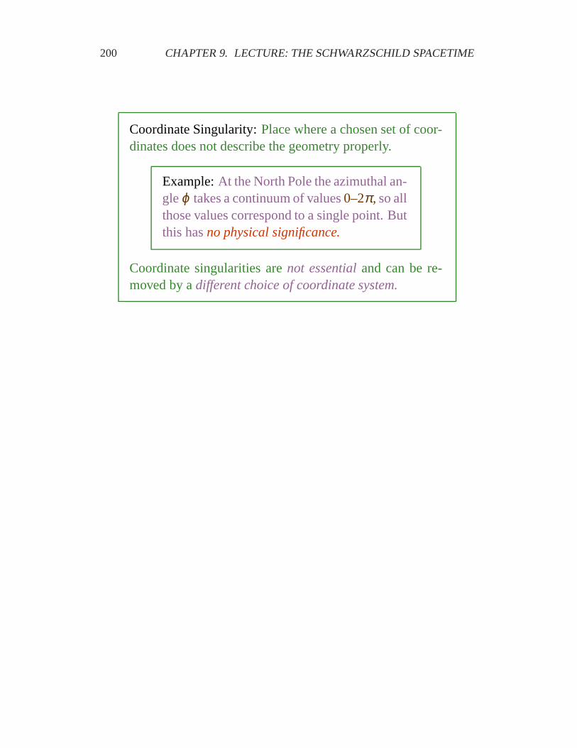
Coordinate Singularity:Place where a chosen set of coor-dinates does not describe the geometry properly.
Example:At the North Pole the azimuthal an-gleϕ takes a continuum of values0–2π , so allthose values correspond to a single point. Butthis hasno physical significance.
Coordinate singularities arenot essentialand can be re-moved by adifferent choice of coordinate system.
9.1. THE FORM OF THE METRIC 201
9.1.1 Measuring Distance and Time
What is the physical meaning of the coordinates(t, r,θ ,ϕ)?
• We may assign a practical definition to the radial coordinate r by
1. Enclosing the origin of our Schwarzschild spacetime in aseries of concentric spheres,
2. Measuring for each sphere a surface area (conceptually bylaying measuring rods end to end),
3. Assigning a radial coordinater to that sphere usingArea =4πr2.
• Then we can use distances and trigonometry to define the angu-lar coordinate variablesθ andϕ.
• Finally we can define coordinate timet in terms of clocks at-tached to the concentric spheres.
For Newtonian theory with its implicit assumption thatevents occur on a passive background of euclidean spaceand constantly flowing time, that’s the whole story.
202 CHAPTER 9. LECTURE: THE SCHWARZSCHILD SPACETIME
But in curved Schwarzschild spacetime
• The coordinates(t, r,θ ,ϕ) provide a global reference frame foran observer making measurements an infinite distance from thegravitational source of the Schwarzschild spacetime.
• However, physical quantities measured by arbitary observers arenot specified directly by these coordinates but ratherphysicalquantitites must be computed from the metric.

9.1. THE FORM OF THE METRIC 203
Proper and Coordinate Distances
Consider distance measured in the radial direction. Set
dt = dθ = dϕ = 0
in the line element to obtain an interval of radial distance
ds2 =−(
1− 2Mr
)
dt2 +
(
1− 2Mr
)−1
dr2+ r2dθ2 + r2sin2θdϕ2
︸ ︷︷ ︸
set t,θ ,ϕ to constants→ dt=dθ=dϕ=0
ds=dr
√
1− 2GMrc2
,
• In this expression we term
1. dstheproper distanceand
2. dr thecoordinate distance.
• The physical interval in the radial direction measured by alocalobserver is given by the proper distanceds, notby dr.
• GM/rc2 is a measure of the strength of gravity, so the properdistance and coordinate distance are equivalent only if gravity isnegligibly weak, either because
1. The sourceM is weak, or
2. We are a very large coordinate distancer from the source.
204 CHAPTER 9. LECTURE: THE SCHWARZSCHILD SPACETIME
Asymptotically
flat space
(dr ~ ds)
Asymptotically
flat space
(dr ~ ds)
ds
dr
C1
C2
C3C4
(1-2M/r)-1/2
Curved space
(dr < ds )
Flat space
(dr = ds)
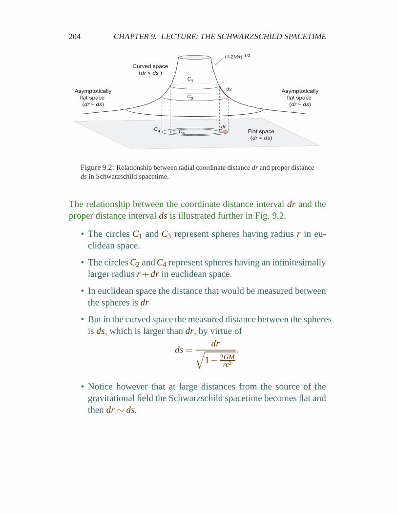
Figure 9.2:Relationship between radial coordinate distancedr and proper distanceds in Schwarzschild spacetime.
The relationship between the coordinate distance intervaldr and theproper distance intervalds is illustrated further in Fig. 9.2.
• The circlesC1 andC3 represent spheres having radiusr in eu-clidean space.
• The circlesC2 andC4 represent spheres having an infinitesimallylarger radiusr +dr in euclidean space.
• In euclidean space the distance that would be measured betweenthe spheres isdr
• But in the curved space the measured distance between the spheresis ds, which is larger thandr, by virtue of
ds=dr
√
1− 2GMrc2
,
• Notice however that at large distances from the source of thegravitational field the Schwarzschild spacetime becomes flat andthendr ∼ ds.
9.1. THE FORM OF THE METRIC 205
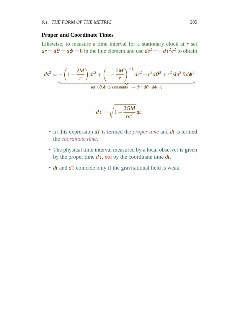
Proper and Coordinate Times
Likewise, to measure a time interval for a stationary clock at r setdr = dθ = dϕ = 0 in the line element and useds2 =−dτ2c2 to obtain
ds2 =−(
1− 2Mr
)
dt2 +
(
1− 2Mr
)−1
dr2+ r2dθ2 + r2sin2θdϕ2
︸ ︷︷ ︸
set r,θ ,ϕ to constants→ dr=dθ=dϕ=0
dτ =
√
1− 2GMrc2 dt.
• In this expressiondτ is termed theproper timeanddt is termedthecoordinate time.
• The physical time interval measured by a local observer is givenby the proper timedτ, notby the coordinate timedt.
• dt anddτ coincide only if the gravitational field is weak.
206 CHAPTER 9. LECTURE: THE SCHWARZSCHILD SPACETIME
Thus we see that for the gravitational field outside a spher-ical mass distribution
• The coordinatesr andt correspond directly to physi-cal distance and time in Newtonian gravity.
• In general relativity the physical (proper) distancesand timesmust be computed from the metric and arenot given directly by the coordinates.
• Only in regions of spacetime where gravity is veryweak do we recover the Newtonian interpretation.
This is as it should be:The goal of relativity is to makethe laws of physics independent of the coordinate systemin which they are formulated.
9.1. THE FORM OF THE METRIC 207
The coordinates in a physical theory are like street num-bers.
• They provide a labeling that locates points in a space,but knowing the street numbers is not sufficient todetermine distances.
• We can’t answer the question of whether the distancebetween 36th Street and 37th street is the same as thedistance between 40th Street and 41st Street until weknow whether the streets are equally spaced.
• We must compute distances from ametric that givesa distance-measuring prescription.
– Streets that are always equally spaced corre-spond to a “flat” space.
– Streets with irregular spacing correspond toa position-dependent metric and thus to a“curved” space.
For the flat space the difference in street number cor-responds directly (up to a scale) to a physical dis-tance, but in the more general (curved) case it doesnot.
208 CHAPTER 9. LECTURE: THE SCHWARZSCHILD SPACETIME
9.1.2 Embedding Diagrams
It is sometimes useful to form a mental image of the struc-ture for a curved space by embedding the space or a subsetof its dimensions in 3-D euclidean space.
Such embedding diagrams can be misleading, as illustrated well bythe case of a cylinder embedded in 3-D euclidean space, whichsug-gests that a cylinder is curved. But it isn’t:
• The cylinder is intrinsically a flat 2-D surface:(a) cut it and roll itout into a plane, or (b) calculate its vanishing gaussian curvature.
• The cylinder hasno intrinsic curvature;the appearance of cur-vature derives entirely from the embedding in 3-D space and istermedextrinsic curvature.
Nevertheless, the image of the cylinder embedded in 3D euclideanspace is a useful representation of many properties associated with acylinder.
9.1. THE FORM OF THE METRIC 209
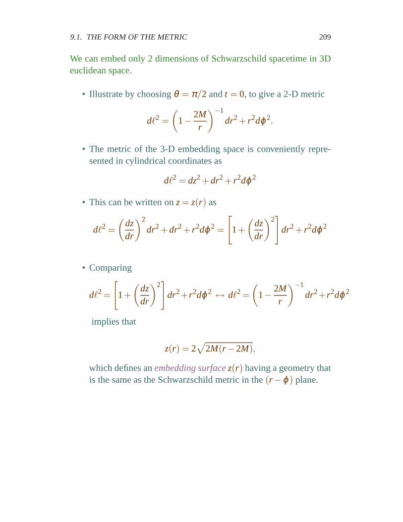
We can embed only 2 dimensions of Schwarzschild spacetime in3Deuclidean space.
• Illustrate by choosingθ = π/2 andt = 0, to give a 2-D metric
dℓ2 =
(
1− 2Mr
)−1
dr2+ r2dϕ2.
• The metric of the 3-D embedding space is conveniently repre-sented in cylindrical coordinates as
dℓ2 = dz2+dr2+ r2dϕ2
• This can be written onz= z(r) as
dℓ2 =
(dzdr
)2
dr2+dr2+ r2dϕ2 =
[
1+
(dzdr
)2]
dr2+ r2dϕ2
• Comparing
dℓ2 =
[
1+
(dzdr
)2]
dr2+r2dϕ2 ↔ dℓ2 =
(
1− 2Mr
)−1
dr2+r2dϕ2
implies that
z(r) = 2√
2M(r−2M),
which defines anembedding surfacez(r) having a geometry thatis the same as the Schwarzschild metric in the(r−ϕ) plane.
210 CHAPTER 9. LECTURE: THE SCHWARZSCHILD SPACETIME
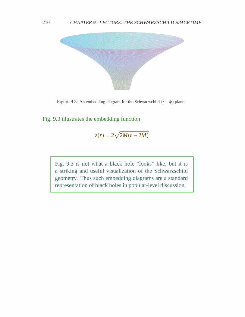
Figure 9.3:An embedding diagram for the Schwarzschild(r−ϕ) plane.
Fig. 9.3 illustrates the embedding function
z(r) = 2√
2M(r−2M)
Fig. 9.3 is not what a black hole “looks” like, but it isa striking and useful visualization of the Schwarzschildgeometry. Thus such embedding diagrams are a standardrepresentation of black holes in popular-level discussion.
9.1. THE FORM OF THE METRIC 211
r
t
Light ray
So
urc
e
Sch
wa
rzsch
ild r
ad
ius
Dis
tan
t o
bse
rve
r
r = 2M0 r = R1
Emission of light
with frequency ω0
Detection of light
with frequency ω
r ~
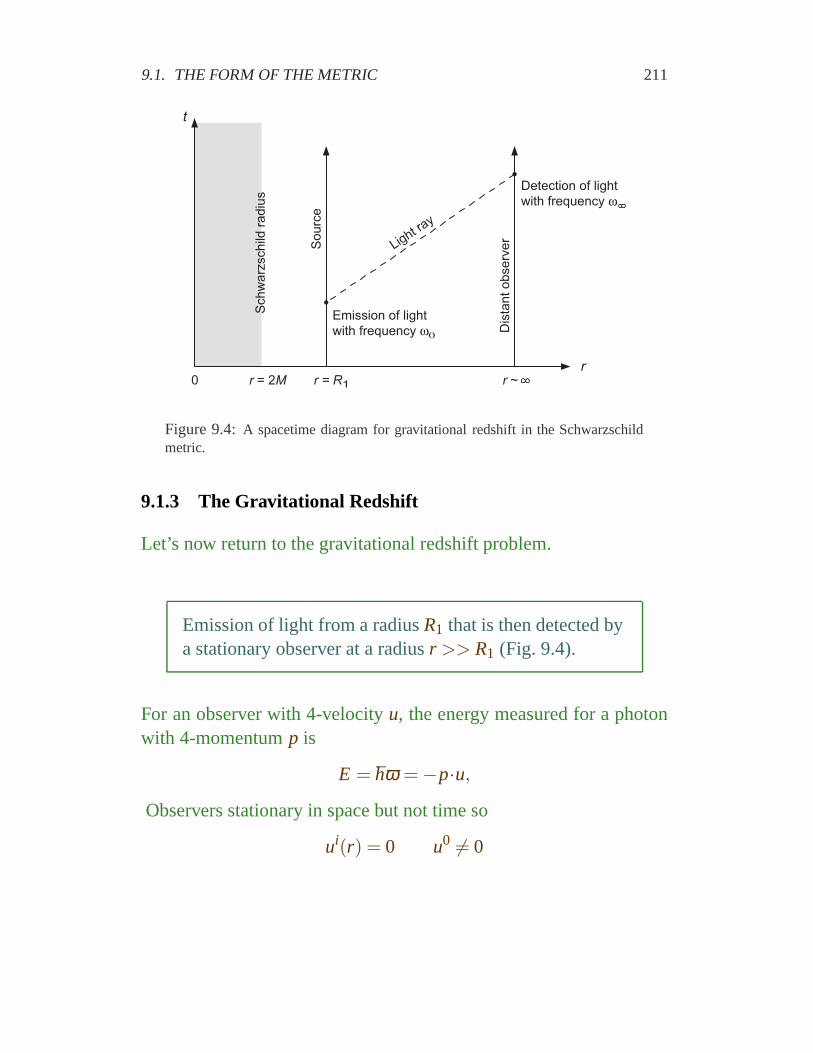
Figure 9.4:A spacetime diagram for gravitational redshift in the Schwarzschildmetric.
9.1.3 The Gravitational Redshift
Let’s now return to the gravitational redshift problem.
Emission of light from a radiusR1 that is then detected bya stationary observer at a radiusr >> R1 (Fig. 9.4).
For an observer with 4-velocityu, the energy measured for a photonwith 4-momentump is
E = h̄ω =−p·u,
Observers stationary in space but not time so
ui(r) = 0 u0 6= 0

212 CHAPTER 9. LECTURE: THE SCHWARZSCHILD SPACETIME
Thus the 4-velocity normalization gives
u·u = gµν(x)dxµ
dτdxν
dτ= g00(x)u
0(r)u0(r) =−1.︸ ︷︷ ︸
Solve foru0(r)
and we obtain
u0(r) =
√
−1g00
=
(
1− 2Mr
)−1/2
.
Symmetry: Schwarzschild metricindependent of time,which implies the existence of aKilling vector
ξ µ = (t, r,θ ,ϕ) = (1,0,0,0)
associated with symmetry under time displacement.
Thus, for a stationary observer at a distancer ,
uµ(r) =
((
1− 2Mr
)−1/2
, 0, 0, 0
)
=
(
1− 2Mr
)−1/2
ξ µ .
The energy of the photon measured atr by stationary observer is
h̄ω(r) =−p·u =−(
1− 2Mr
)−1/2
(ξ ·p)r
9.1. THE FORM OF THE METRIC 213
But ξ ·p is conserved along the photon geodesic(ξ is aKilling vector) soξ ·p is in fact independent ofr .
Therefore,
h̄ω0≡ h̄ω(R1) =−(
1− 2MR1
)−1/2
(ξ ·p)
h̄ω∞ ≡ h̄ω(r → ∞) =−(ξ ·p),
and fromh̄ω∞/h̄ω0 we obtain immediately a gravitational redshift
ω∞ = ω0
(
1− 2MR1
)1/2
.
We have made no weak-field assumptions so this resultshould be valid for weak and strong fields.
For weak fields2M/R1 is small, the square root can be expanded, andtheG andc factors restored to give
ω∞ ≃ ω0
(
1− GMR1c2
)
(valid for weak fields)
which is the result derived earlier using the equivalence principle.
By viewing ω as defining clock ticks, the redshift mayalso be interpreted as agravitational time dilation.
214 CHAPTER 9. LECTURE: THE SCHWARZSCHILD SPACETIME
9.1.4 Particle Orbits in the Schwarzschild Metric
Symmetries of the Schwarzschild metric:
1. Time independence→ Killing vector ξt = (1,0,0,0)
2. No dependence onϕ → Killing vector ξϕ = (0,0,0,1)
3. Additional Killing vectors associated with full rotational sym-metry (won’t need in following).
Conserved quantities associated with these Killing vectors:
ε ≡−ξt ·u =
(
1− 2Mr
)dtdτ
ℓ≡ ξϕ ·u = r2sin2θdϕdτ
.
Physical interpretation:
• At low velocitiesℓ∼ (orbital angular momentum / unit rest mass)
• SinceE = p0 = mu0 = mdt/dτ ,
Limr→∞
ε =dtdτ
=Em
andε ∼ energy / (unit rest mass)at large distance.
Also we have the velocity normalization constraint
u·u = gµνuµuν =−1.
9.1. THE FORM OF THE METRIC 215
Conservation of angular momentum confines the particlemotion to a plane, which we conveniently take to be theequatorial plane withθ = π
2 implying thatu2≡ uθ = 0.
Then writing the velocity constraint
gµνuµuν =−1.
out in the metric gives
−(
1− 2Mr
)
(u0)2 +
(
1− 2Mr
)−1
(u1)2 + r2(u3)2 =−1.
which we may rewrite using
uµ =
(dx0
dτ,dx1
dτ,dx2
dτ,dx3
dτ
)
ε =
(
1− 2Mr
)dtdτ
ℓ = r2sin2θdϕdτ
.
in the form
ε2−12
=12
(drdτ
)2
+12
[(
1− 2Mr
)(ℓ2
r2 +1
)
−1
]
.
216 CHAPTER 9. LECTURE: THE SCHWARZSCHILD SPACETIME
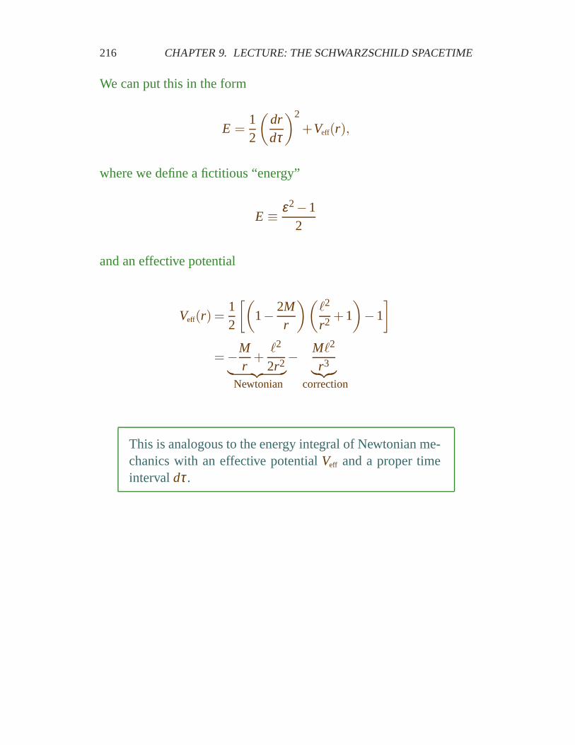
We can put this in the form
E =12
(drdτ
)2
+Veff(r),
where we define a fictitious “energy”
E ≡ ε2−12
and an effective potential
Veff(r) =12
[(
1− 2Mr
)(ℓ2
r2 +1
)
−1
]
=−Mr
+ℓ2
2r2︸ ︷︷ ︸
Newtonian
− Mℓ2
r3︸︷︷︸
correction
This is analogous to the energy integral of Newtonian me-chanics with an effective potentialVeff and a proper timeintervaldτ.
9.1. THE FORM OF THE METRIC 217
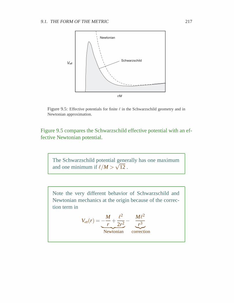
Veff
r/M
Newtonian
Schwarzschild
Figure 9.5:Effective potentials for finiteℓ in the Schwarzschild geometry and inNewtonian approximation.
Figure 9.5 compares the Schwarzschild effective potentialwith an ef-fective Newtonian potential.
The Schwarzschild potential generally has one maximumand one minimum ifℓ/M >
√12 .
Note the very different behavior of Schwarzschild andNewtonian mechanics at the origin because of the correc-tion term in
Veff(r) =−Mr
+ℓ2
2r2︸ ︷︷ ︸
Newtonian
− Mℓ2
r3︸︷︷︸
correction
218 CHAPTER 9. LECTURE: THE SCHWARZSCHILD SPACETIME
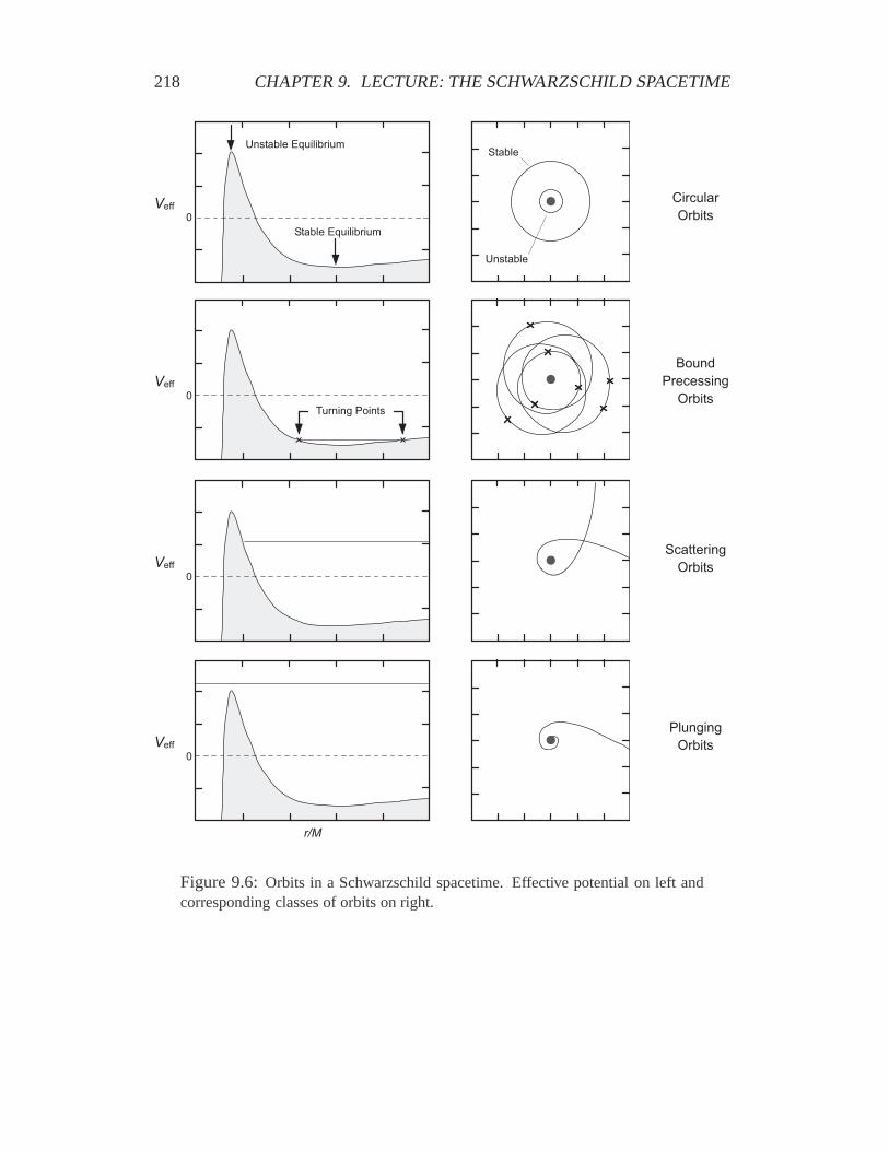
Veff
Veff
0
0
Stable Equilibrium
Unstable Equilibrium
Veff
0
Veff
0
Turning Points
r/M
Circular
Orbits
Bound
Precessing
Orbits
Scattering
Orbits
Plunging
Orbits
Unstable
Stable
Figure 9.6:Orbits in a Schwarzschild spacetime. Effective potential on left andcorresponding classes of orbits on right.
9.1. THE FORM OF THE METRIC 219
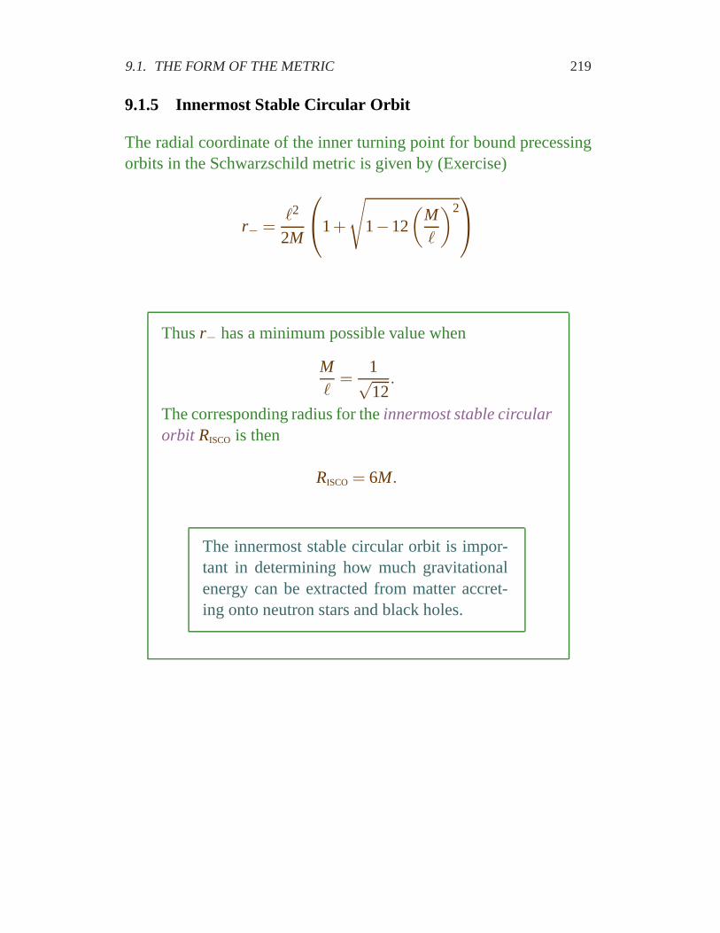
9.1.5 Innermost Stable Circular Orbit
The radial coordinate of the inner turning point for bound precessingorbits in the Schwarzschild metric is given by (Exercise)
r− =ℓ2
2M
1+
√
1−12
(Mℓ
)2
Thusr− has a minimum possible value when
Mℓ
=1√12
.
The corresponding radius for theinnermost stable circularorbit RISCO is then
RISCO = 6M.
The innermost stable circular orbit is impor-tant in determining how much gravitationalenergy can be extracted from matter accret-ing onto neutron stars and black holes.
220 CHAPTER 9. LECTURE: THE SCHWARZSCHILD SPACETIME
r+
δφ
r-
r+
r-
r+
r-
r+
r-
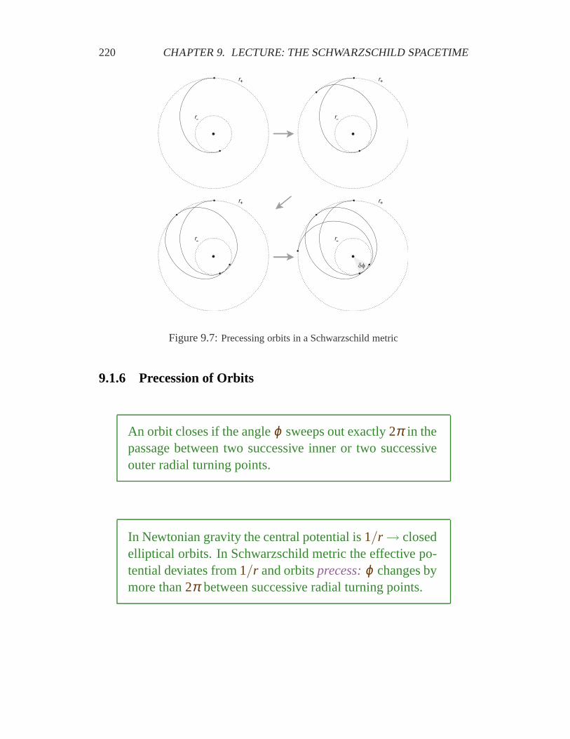
Figure 9.7:Precessing orbits in a Schwarzschild metric
9.1.6 Precession of Orbits
An orbit closes if the angleϕ sweeps out exactly2π in thepassage between two successive inner or two successiveouter radial turning points.
In Newtonian gravity the central potential is1/r → closedelliptical orbits. In Schwarzschild metric the effective po-tential deviates from1/r and orbitsprecess:ϕ changes bymore than2π between successive radial turning points.
9.1. THE FORM OF THE METRIC 221
To investigate this precession quantitatively we require an expressionfor dϕ/dr. From the energy equation
drdτ
=±√
2(E−Veff(r)),
and from the conservation equation forℓ,
dϕdτ
=ℓ
r2sin2θ.
Combinine, recalling that we are choosing an orbital planeθ = π2 ,
dϕdr
=dϕ/dτdr/dτ
=± ℓ
r2√
2(E−Veff(r))
=± ℓ
r2
[
2E−(
1− 2Mr
)(
1+ℓ2
r2
)
+1
]−1/2
=± ℓ
r2
[
ε2−(
1− 2Mr
)(
1+ℓ2
r2
)]−1/2
,
where we have usedE = 12(ε
2−1).
222 CHAPTER 9. LECTURE: THE SCHWARZSCHILD SPACETIME
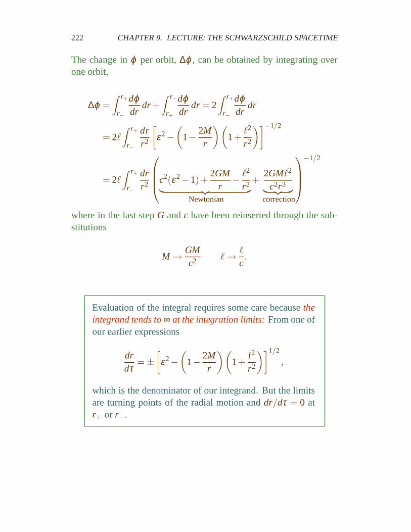
The change inϕ per orbit,∆ϕ, can be obtained by integrating overone orbit,
∆ϕ =
∫ r+
r−
dϕdr
dr +
∫ r−
r+
dϕdr
dr = 2∫ r+
r−
dϕdr
dr
= 2ℓ∫ r+
r−
drr2
[
ε2−(
1− 2Mr
)(
1+ℓ2
r2
)]−1/2
= 2ℓ∫ r+
r−
drr2
c2(ε2−1)+2GM
r− ℓ2
r2︸ ︷︷ ︸
Newtonian
+2GMℓ2
c2r3︸ ︷︷ ︸
correction
−1/2
where in the last stepG andc have been reinserted through the sub-stitutions
M→ GMc2 ℓ→ ℓ
c,
Evaluation of the integral requires some care becausetheintegrand tends to∞ at the integration limits:From one ofour earlier expressions
drdτ
=±[
ε2−(
1− 2Mr
)(
1+l2
r2
)]1/2
,
which is the denominator of our integrand. But the limitsare turning points of the radial motion anddr/dτ = 0 atr+ or r−.
9.1. THE FORM OF THE METRIC 223
In the Solar System and most other applications the valuesof ∆ϕ are very small, so it is sufficient to keep only termsof order1/c2 beyond the Newtonian approximation.
Expanding the integrand and evaluating the integral with due care(Exercise) yields
Precession angle= δϕ ≡ ∆ϕ−2π
≃ 6π(
GMcℓ
)2
rad/orbit.
This may be expressed in more familiar classical orbital parameters:
• In Newtonian mechanicsL = mr2ω , whereL is the angular mo-mentum andω the angular frequency.
• For Kepler orbits
ℓ2 =
(Lm
)2
=
(
r2dϕdτ
)2
≃(
r2dϕdt
)2
= GMa(1−e2),
wheree is the eccentricity anda is the semimajor axis.
This permits us to write
δϕ =6πGM
ac2(1−e2)
= 1.861×10⁻⁷(
MM⊙
)(AUa
)1
1−e2 rad/orbit,
224 CHAPTER 9. LECTURE: THE SCHWARZSCHILD SPACETIME
The form of
δϕ =6πGM
ac2(1−e2)
shows explicitly that the amount of relativistic precession is enhancedby
• largeM for the central mass,
• tight orbits (small values ofa),
• large eccentricitiese.
The precession observed for most objects is small.
• Precession of Mercury’s orbit in the Sun’s gravitational field be-cause of general relativistic effects is observed to be43 arcsec-onds per century.
• The orbit of the Binary Pulsar precesses by about4.2 degreesper year.
The precise agreement of both of these observations with thepredic-tions of general relativity is a strong test of the theory.
9.1. THE FORM OF THE METRIC 225
9.1.7 Escape Velocity in the Schwarzschild Metric
Consider a stationary observer at a Schwarzschild radialcoordinateR who launches a projectile radially with avelocity v such that the projectile reaches infinity withzero velocity. This defines the escape velocity in theSchwarzschild metric.
• The projectile follows a radial geodesic since thereare no forces acting on it
• The energy per unit rest mass isε and it is conserved(time invariance of metric).
• At infinity ε = 1, since then the particle is at rest andthe entire energy is rest mass energy. Thusε = 1 atall times.
If uobs is the 4-velocity of the stationary observer, the energy measuredby the observer is
E =−p·uobs =−mu·uobs
=−mgµνuµuνobs
=−mg00u0u0
obs,
wherep = mu, with p the 4-momentum andm the rest mass, and thelast step follows because the observer is stationary. But
g00 =−(1− 2M
r
)
︸ ︷︷ ︸
From metric
u0obs=
(1− 2M
R
)−1/2
︸ ︷︷ ︸
Stationary observer
u0 =(1− 2M
r
)−1
︸ ︷︷ ︸
Fromε = (1− 2Mr )u0 = 1
226 CHAPTER 9. LECTURE: THE SCHWARZSCHILD SPACETIME
Therefore,
E =−mg00u0u0
obs
= m(1− 2M
r
)(1− 2M
r
)−1(1− 2M
r
)−1/2
= m(1− 2M
R
)−1/2
But in the observer’s rest frame
E = mγ = m(1−v2)−1/2
so comparison yields2M/R= v2 and thus
vesc=
√
2MR
Notice that
• This, coincidentally, is the same result as for Newtonian theory.
• At the Schwarzschild radiusR= rS = 2M, the escape velocity isequal toc.
This is the first hint of anevent horizonin the Schwarzschild space-time.
9.1. THE FORM OF THE METRIC 227
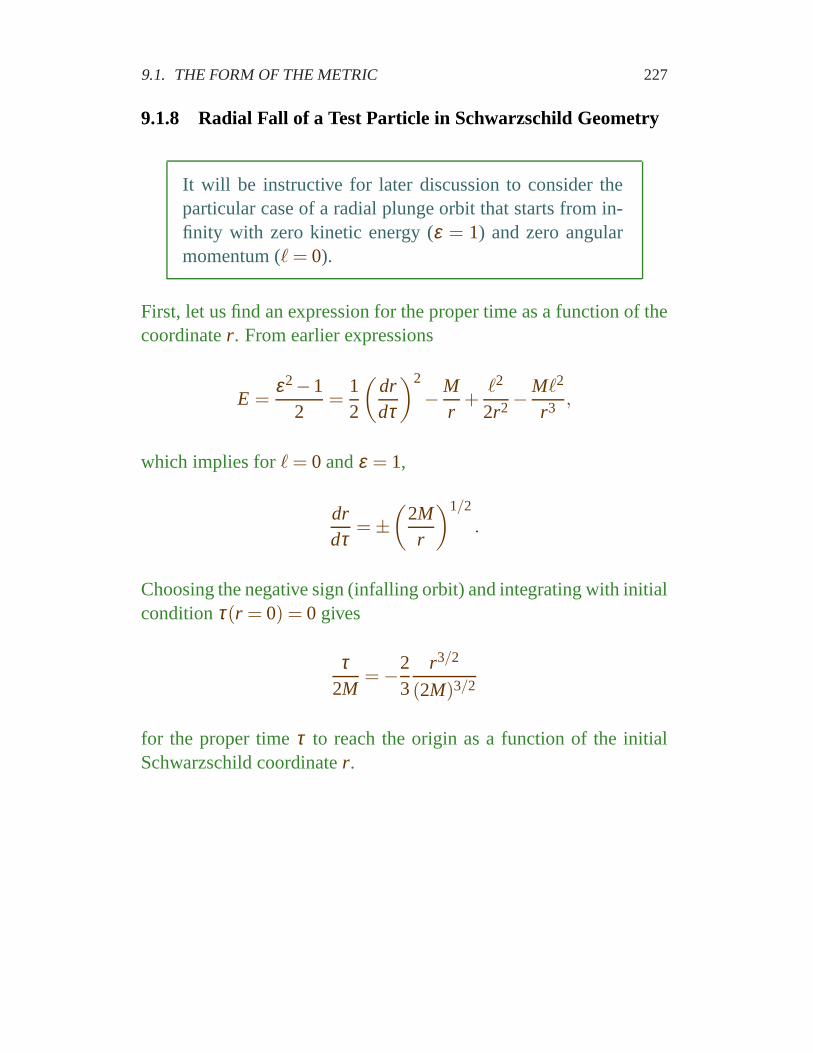
9.1.8 Radial Fall of a Test Particle in Schwarzschild Geometry
It will be instructive for later discussion to consider theparticular case of a radial plunge orbit that starts from in-finity with zero kinetic energy (ε = 1) and zero angularmomentum (ℓ = 0).
First, let us find an expression for the proper time as a function of thecoordinater . From earlier expressions
E =ε2−1
2=
12
(drdτ
)2
−Mr
+ℓ2
2r2−Mℓ2
r3 ,
which implies forℓ = 0 andε = 1,
drdτ
=±(
2Mr
)1/2
.
Choosing the negative sign (infalling orbit) and integrating with initialconditionτ(r = 0) = 0 gives
τ2M
=−23
r3/2
(2M)3/2
for the proper timeτ to reach the origin as a function of the initialSchwarzschild coordinater .
228 CHAPTER 9. LECTURE: THE SCHWARZSCHILD SPACETIME
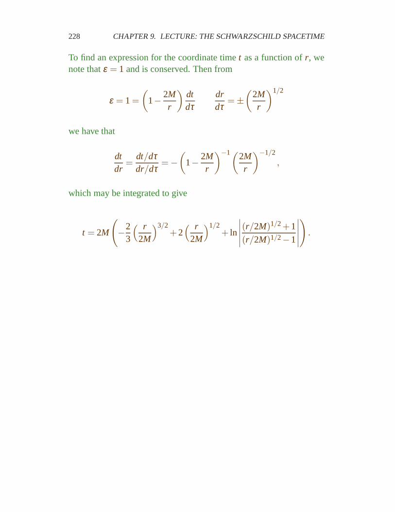
To find an expression for the coordinate timet as a function ofr , wenote thatε = 1 and is conserved. Then from
ε = 1 =
(
1− 2Mr
)dtdτ
drdτ
=±(
2Mr
)1/2
we have that
dtdr
=dt/dτdr/dτ
=−(
1− 2Mr
)−1(2Mr
)−1/2
,
which may be integrated to give
t = 2M
(
−23
( r2M
)3/2+2( r
2M
)1/2+ ln
∣∣∣∣∣
(r/2M)1/2+1
(r/2M)1/2−1
∣∣∣∣∣
)
.
9.1. THE FORM OF THE METRIC 229
r /M
Proper
time τ
Schwarzschild
coordinate time t
-Time/M
rS = 2M
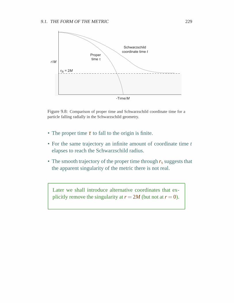
Figure 9.8:Comparison of proper time and Schwarzschild coordinate time for aparticle falling radially in the Schwarzschild geometry.
• The proper timeτ to fall to the origin is finite.
• For the same trajectory an infinite amount of coordinate time telapses to reach the Schwarzschild radius.
• The smooth trajectory of the proper time throughrS suggests thatthe apparent singularity of the metric there is not real.
Later we shall introduce alternative coordinates that ex-plicitly remove the singularity atr = 2M (but not atr = 0).
230 CHAPTER 9. LECTURE: THE SCHWARZSCHILD SPACETIME
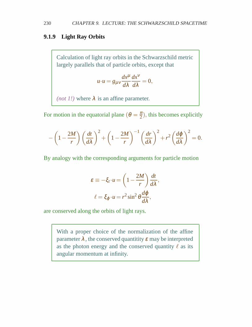
9.1.9 Light Ray Orbits
Calculation of light ray orbits in the Schwarzschild metriclargely parallels that of particle orbits, except that
u·u = gµνdxµ
dλdxν
dλ= 0,
(not 1!) whereλ is an affine parameter.
For motion in the equatorial plane(θ = π2), this becomes explicitly
−(
1− 2Mr
)(dtdλ
)2
+
(
1− 2Mr
)−1( drdλ
)2
+ r2(
dϕdλ
)2
= 0.
By analogy with the corresponding arguments for particle motion
ε ≡−ξt ·u=
(
1− 2Mr
)dtdλ
,
ℓ = ξϕ ·u= r2sin2θdϕdλ
,
are conserved along the orbits of light rays.
With a proper choice of the normalization of the affineparameterλ , the conserved quantitityε may be interpretedas the photon energy and the conserved quantityℓ as itsangular momentum at infinity.
9.1. THE FORM OF THE METRIC 231
Veff 0
+
−
Veff 0
+
−
Veff 0
+
−
r orbits
Circular
orbit
Scattering
orbit
Plunging
orbit
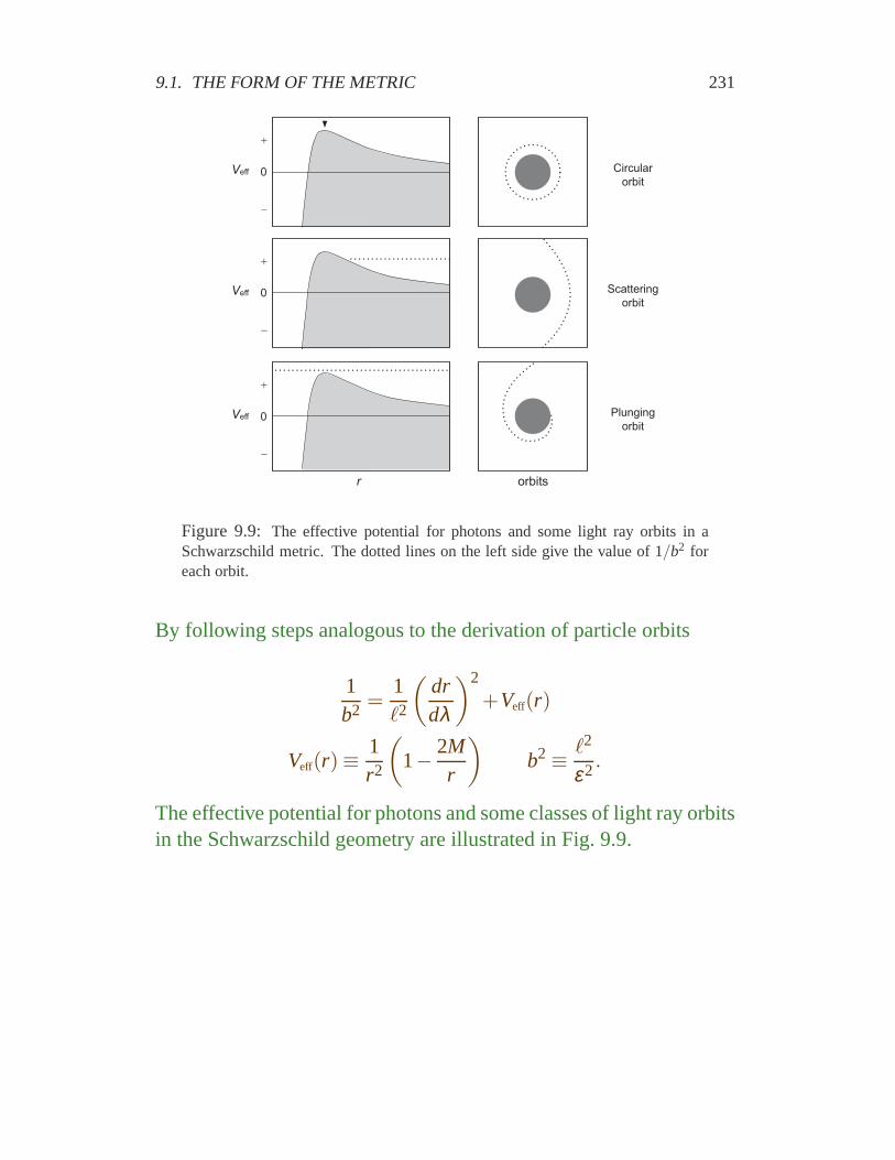
Figure 9.9: The effective potential for photons and some light ray orbits in aSchwarzschild metric. The dotted lines on the left side givethe value of 1/b2 foreach orbit.
By following steps analogous to the derivation of particle orbits
1b2 =
1ℓ2
(drdλ
)2
+Veff(r)
Veff(r)≡1r2
(
1− 2Mr
)
b2≡ ℓ2
ε2.
The effective potential for photons and some classes of light ray orbitsin the Schwarzschild geometry are illustrated in Fig. 9.9.
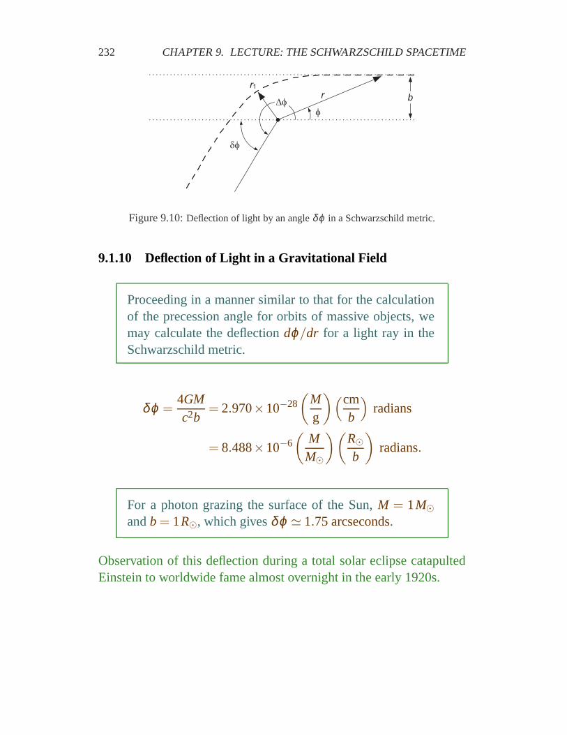
232 CHAPTER 9. LECTURE: THE SCHWARZSCHILD SPACETIME
∆φφ
δφ
rr1
b
Figure 9.10:Deflection of light by an angleδϕ in a Schwarzschild metric.
9.1.10 Deflection of Light in a Gravitational Field
Proceeding in a manner similar to that for the calculationof the precession angle for orbits of massive objects, wemay calculate the deflectiondϕ/dr for a light ray in theSchwarzschild metric.
δϕ =4GMc2b
= 2.970×10⁻²⁸(
Mg
)(cmb
)
radians
= 8.488×10⁻⁶(
MM⊙
)(R⊙b
)
radians.
For a photon grazing the surface of the Sun,M = 1M⊙andb = 1R⊙, which givesδϕ ≃ 1.75 arcseconds.
Observation of this deflection during a total solar eclipse catapultedEinstein to worldwide fame almost overnight in the early 1920s.