Chapter 7Boundary Layer Theory

We have seen in Chap.6 that singularly perturbed problems can have co-existingregular and singular solutions that scale differently as ε → 0. In the context ofphysical systemsdescribedbydifferential equations, such structures yieldmulti-scalephenomena. Everyday life yields countless examples of multi-scale phenomena:violent winds in tornadoes surrounded by relatively calm air over large areas, bandsof wake behind ships moving in otherwise still waters, cracks forming in uniformsolid materials, spots, stripes and other intricate patterns developing in biologicalsystems. In these, and many other contexts, we can separate the behaviour of thesystem into regions of rapid variation of quantities of interest compared to other largerscale regions of slow variation. Models that can capture such diverse behaviours willallow for multiple distinguished limits, describing balances between different sets ofdominant effects in different regions. The relatively narrow regions of rapid variationsare generally called boundary layers.

Although boundary layers were originally formulated to describe problems influid mechanics and aerodynamics [76] (where they generally occur on the boundaryof a solid object passing through a surrounding uniformfluid flow), they also describesolutions in broader sets of contexts.

While attempting to directly find a solution of the full problem on an entire domaindirectly may be very difficult, constructing “partial solutions” on different regionsusing perturbation expansions can be straightforward. Following the approach in-troduced in Sect. 6.5, different dominant balances will re-scale the full model intodifferent forms, leading to different regular or singular solutions. Further analysis isthen needed to assemble the partial solutions into a complete solution of the full prob-lem. This is accomplished through asymptotic matching and leads to this solutionmethodology being called the method of matched asymptotic expansions.

© Springer International Publishing Switzerland 2015T. Witelski and M. Bowen, Methods of Mathematical Modelling,Springer Undergraduate Mathematics Series, DOI 10.1007/978-3-319-23042-9_7

147

148 7 Boundary Layer Theory

7.1 Observing Boundary Layer Structure in Solutions

In order to illustrate the main principles behind boundary layers andmatched asymp-totics, we first consider a problem for which we can express the solution exactly andexamine how it can be separated into pieces stemming from behaviours at differentscales.

Consider the linear, constant coefficient ordinary differential equation

εd2y

dx2+ 2

dy

dx+ y = 0 for ε → 0, (7.1a)

on the domain 0 ≤ x ≤ 1, subject to the boundary conditions

y(0) = 0, y(1) = 1. (7.1b)

Singular behaviour in the solution should be expected since setting ε = 0 in (7.1a)reduces the equation to a first order ODE, whose solution can satisfy only one of theboundary conditions.

The exact solution of (7.1) for any ε > 0 is given by

y(x) =exp

(−1+√1−ε

εx)

− exp(−1−√

1−εε

x)

exp(−1+√

1−εε

)− exp

(−1−√1−ε

ε

) (7.2)

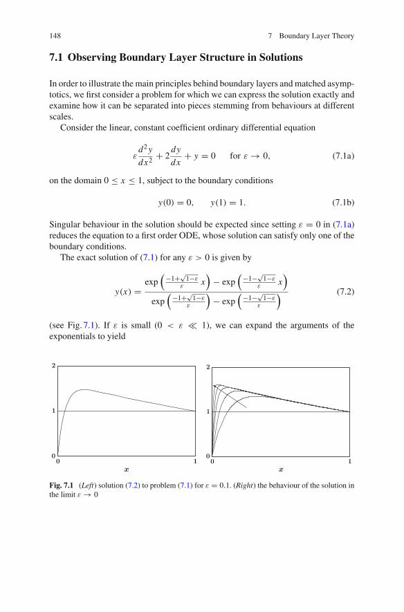
(see Fig. 7.1). If ε is small (0 < ε � 1), we can expand the arguments of theexponentials to yield

Fig. 7.1 (Left) solution (7.2) to problem (7.1) for ε = 0.1. (Right) the behaviour of the solution inthe limit ε → 0

7.1 Observing Boundary Layer Structure in Solutions 149

y(x) =exp

(−[ 1

2 + ε8 + · · · ] x

)− exp

(−[ 2

ε− 1

2 + · · · ] x)

exp(−[ 1

2 + ε8 + · · · ]

)− exp

(−[ 2

ε− 1

2 + · · · ])

∼ exp(− 1

2 x) − exp

(− 2ε

x)

exp(− 1

2

) − exp(− 2

ε

) , (7.3)

The size of the domain is independent of ε, and hence one of the spatial scales shouldbe x = O(1) as ε → 0, as represented by the e−x/2 term in (7.3). The other termthere depends on a more rapidly varying spatial scale, x/ε, in which a small (O(ε))change in x yields a O(1) change in the solution. The distinctness of these two scalesmakes it possible to construct the solution to (7.1) by seeking its dependence on eachscale separately.

Each spatial scale in the problem is associated with a limiting process for thesolution of (7.1) as ε → 0. Fixing x = O(1) in the range 0 < x ≤ 1 gives

limε→0

y(x) ∼ e−x/2 − e.s.t.

e−1/2 − e.s.t.∼ e(1−x)/2, (7.4)

where “e.s.t.” refers to exponentially small terms, of the form e−α/ε for α > 0, thatare smaller than all algebraic powers of ε (εn � e−α/ε for ε → 0) and are treated asnegligible in this context. This limiting form of the solution satisfies the boundarycondition at x = 1, but not the one at x = 0 (7.1b).

Note that we have excluded the case x = 0 from consideration in (7.4) so thate−2x/ε is indeed exponentially small. If instead, we consider a small neighbourhoodof the origin, 0 ≤ x = O(ε), then we must take the dual limit ε → 0 and x → 0with the ratio X = x/ε held fixed. In terms of the new spatial variable X , the limitof (7.3) now becomes

limε→0

y ∼ e−εX/2 − e−2X

e−1/2 − e−2/ε ∼ e1/2(1 − e−2X ). (7.5)

This limiting form satisfies the boundary condition at x = 0 (X = 0). The boundarycondition at x = 1 is not satisfied, but since the right hand boundary position,corresponding to X = 1/ε, violates the assumption X = O(1) made in taking thelimit, agreement should not have been expected.

Similar examples are often used in analysis [21] to illustrate functions that havenon-uniform convergence. In the present context, we see that different limiting prop-erties of the solution are captured by different limiting processes. For the majorityof the domain (here, where x = O(1)), the solution is given by (7.4) and is calledthe outer solution. In contrast, in the boundary layer, or inner domain, the solutionexhibits singular behaviour that cannot be captured by the outer solution. In thisexample, the inner solution in the boundary layer close to x = 0 has a singularderivative, dy/dx = O(ε−1) → ∞ as ε → 0.

150 7 Boundary Layer Theory

It is also worth mentioning that problems featuring a separation of scales can beextremely difficult to compute numerically (typically referred to as stiff problems). Incontrast, solutions of these problems can often be very accurately obtained in termsof inner and outer solutions using perturbation methods.

7.2 Asymptotics of the Outer and Inner Solutions

We now discuss the construction of solutions to singular perturbation problems bycalculating perturbation expansions for the outer and inner solutions.

We shall continue to use problem (7.1a, 7.1b) to illustrate the methodology. Webegin by attempting to find the outer solution on the outer domain, 0 < x ≤ 1, inwhich we assume that y(x) and all of its derivatives are bounded, smooth and O(1).We assume y(x) can be expanded as a regular perturbation expansion of the form

y(x) ∼ y0(x) + εy1(x) + ε2y2(x) + · · · as ε → 0. (7.6)

Similar to the approach used for (6.24), we substitute this expansion into (7.1a, 7.1b)and separate terms in powers of ε → 0 yielding the system of sub-problems

O(ε0) : 2y′0 + y0 = 0 y0(1) = 1,

O(ε1) : 2y′1 + y1 = −y′′

0 y1(1) = 0,O(ε2) : 2y′

2 + y2 = −y′′1 y2(1) = 0,

(7.7)

and so on for higher powers of ε. Note that the boundary condition at x = 0 from(7.1b) is not included above since x = 0 is not within the outer domain. Solving theO(1) problem gives the leading order outer solution

y0(x) = e(1−x)/2, (7.8)

which reproduces (7.4). Additional terms in the expansion can be constructed byworking through the higher order sub-problems in (7.7) in sequence.

We now turn our attention to constructing the solution in the inner region, cor-responding to having x = O(ε). Introducing the rescaling x = εX and writingy(x) = Y (X) transforms (7.1a) to

d2Y

d X2 + 2dY

d X+ εY = 0, (7.9)

with the boundary condition (7.1b) becoming Y (0) = 0. Seeking the solution in theform of a regular expansion, Y (X) = Y0(X) + εY1 + ε2Y2(X) + · · · , yields theleading order O(1) problem

Y ′′0 + 2Y ′

0 = 0, Y0(0) = 0, (7.10)

7.2 Asymptotics of the Outer and Inner Solutions 151

with solutionY0(X) = A(1 − e−2X ). (7.11)

Note that one constant, A, remains undetermined in the solution since the ODE in(7.10) is second order, but we are only imposing one side condition. The solutionsof the higher order terms, Yn(X) will similarly add one new undetermined constantat each order in the expansion. Since the inner problem did not uniquely define theinner solution, we examine its relationship with the outer solution in an attempt tofix the unknown constant A.

It is important to note that the inner and outer domains are not mutually exclusiveand are valid on regions broader than the strict prescriptions of their spatial scales(here x = O(ε) and x = O(1) respectively). In the outer solution x is boundedaway from zero, but can become small, say x = O(

√ε) → 0. Likewise, in the inner

solution x should be small, but X = x/ε canbecome large, say X = O(1/√

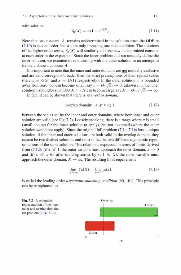
ε) → ∞.In fact, it can be shown that there is an overlap domain,

overlap domain: ε � x � 1, (7.12)

between the scales set by the inner and outer domains, where both inner and outersolution are valid (see Fig. 7.2), Loosely speaking, there is a range where x is small(small enough for the inner solution to apply), but not too small (where the outersolution would not apply). Since the original full problem (7.1a, 7.1b) has a uniquesolution; if the inner and outer solutions are both valid in the overlap domain, theycannot be two distinct solutions and must in fact be two different asymptotic repre-sentations of the same solution. This relation is expressed in terms of limits derivedfrom (7.12): (i) x � 1, the outer variable must approach the inner domain, x → 0and (ii) ε � x (or after dividing across by ε: 1 � X ), the inner variable mustapproach the outer domain, X → ∞. The resulting limit requirement

limX→∞ Y0(X) = lim

x→0y0(x), (7.13)

is called the leading order asymptotic matching condition [60, 101]. This principlecan be paraphrased as

Fig. 7.2 A schematicrepresentation of the inner,outer and overlap domainsfor problem (7.1a, 7.1b)

152 7 Boundary Layer Theory

“The outer limit of the inner solution equals

the inner limit of the outer solution.” (7.14)

Applying (7.13) to Y0 given by (7.11) and y0 by (7.8) yields

limX→∞ A(1 − e−2X ) = A = lim

x→0e(1−x)/2 = e1/2, (7.15)

thereby determining the constant A = e1/2. With this value for A the inner solution(7.11) reproduces the limit (7.5) found from the exact solution.

While we have now determined the leading order inner and outer solutions com-pletely, only a little more work is needed combine the outer and inner solutionsto form a composite representation of the leading order solution, denoted here byycomp(x), valid over the entire domain 0 ≤ x ≤ 1. An appropriate form for ycomp(x)

is given by the expression

ycomp(x) = y0 + Y0 − (overlap from matching), (7.16)

where the overlap is simply the contribution found through matching in (7.15). At aformal level, on most of the domain, we have y ∼ y0, with the inner solution onlybecoming significant in the inner domain. Where Y0 becomes important, we gainequal contributions from both the inner and outer solutions, and so to effectivelyprevent “double-counting”, we must subtract off the overlap.

Another way of expressing (7.16) is to write

ycomp = y0 + YBLC, (7.17)

where the boundary layer correction, YBLC, is the adjustment to the outer solutionmade by the boundary layer to satisfy the boundary condition, with

YBLC ≡ Y0 − (overlap from matching), (7.18)

where we expect YBLC → 0 as X → ∞.Writing the inner solution (7.11) as Y0 = e1/2 − e(1−4x/ε)/2 and using the overlap

from (7.15), the leading order boundary layer correction is

YBLC = e1/2 − e(1−4x/ε)/2 − e1/2 = −e(1−4x/ε)/2, (7.19)

which does indeed vanish as X → ∞. Hence, (7.17) gives the leading order solution

ycomp = e(1−x)/2 − e(1−4x/ε)/2 = e−x/2 − e−2x/ε

e−1/2 , (7.20)

7.2 Asymptotics of the Outer and Inner Solutions 153

on the entire domain 0 ≤ x ≤ 1. This is comparable to the exact solution (7.2), exceptfor the absence of the exponentially small e−2/ε term (which cannot be captured inregular expansions such as (7.6)).

7.3 Constructing Boundary Layer Solutions

The presentation in the previous section made use of some prior knowledge of theform of the solution to reduce the overall problem to that of determining the ex-pansions of the inner and outer solutions. In this section, we describe the furthersteps required to investigate boundary layer problems without any additional giveninformation about the form of the solution.

The full process of constructing a solution involving matched asymptotic expan-sions requires examining the two additional questions:

• What are the scalings for the inner (and outer) solution(s)?• Where are the boundary layer(s) located?

The answers to these questions ultimately determine the form of the overall solution,and control which boundary conditions apply to the inner and outer solutions.

For many singularly perturbed differential equations, solutions can be constructedby a step-by-step process:

(1) The outer solution: If the problem is in standard form, try a regular expansion,y(x) = y0(x) + εy1(x) + · · · , for the outer solution. If all of the boundary con-ditions can be satisfied by this solution, then the problem is complete; otherwise,inner regions will be necessary.

(2) Find the dominant balances: The appropriate forms for all of the regular (outer)and singular (inner) solutions of theODEwill be determined by the distinguishedlimits of the problem. In general, both the independent and dependent variablesmay need to be scaled to obtain all of the dominant balances,

y = εβY (X), X = x − x∗εα

⇔ x = x∗ + εα X, (7.21)

where the powersα, β and the assumedposition of the boundary layer, x∗ must allbe determined (there may be multiple valid locations for x∗). The outer solutionin step (1) assumes α = 0, β = 0.

(3) The inner solution: For the singular distinguished limit, write the problem as arescaled regular problem and seek the solution in the form of an appropriateregular expansion, Y (X) = Y0(X) + εY1(x) + · · · .

(4) Asymptotic matching: Apply asymptotic matching between the inner/outer solu-tions (typically via (7.13)) to confirm the consistencyof the asymptotic expansionand determine any remaining unknown parameters in the solution.

(5) The composite solution: Writing the outer and inner solutions in terms of theoriginal variables and subtracting the overlaps from the matching process to

154 7 Boundary Layer Theory

prevent “double-counting” will produce the leading order solution on the entiredomain (7.16). So, in an example with boundary layers at both the left and rightboundaries, we write

ycomp(x) ∼ y0(x) + Y LBLC + Y R

BLC. (7.22)

This description covers broad classes of problems, but as will be seen, in some cases,steps (2, 3, 4) may become a bit intertwined. We also note:

• When boundary layers are necessary, which boundary conditions apply to theouter solution may not be immediately apparent. Hence a general form for theouter solution will be needed initially.

• The boundary conditions as well as the ODE play a role in determining the dom-inant balances.

• The location of the boundary layer and which boundary conditions apply to theinner solution might not be determined until matching is applied.

• If the inner/outer solutions are notmatchable (either limit does not exist, or equation(7.13) cannot be satisfied) then the assumed choice of boundary layer position x∗or dominant balance may be not be right.

• While the term “boundary layer” stems from the fact that the inner domain oftenoccurs at a boundary, in some cases, they can also occur within the domain of aproblem, in which case they are sometimes called interior layers.

Consequently, the reader should consider steps (1)–(5) as “guidelines” that may needto be adjusted depending on the given problem; this is one of the challenging (andinteresting) points of matched asymptotic expansions.

We use an example to illustrate the aspects of the above procedure. Consider theboundary value problem

εd2y

dx2+ dy

dx= cos x (7.23a)

in the limit ε → 0 on the domain 0 ≤ x ≤ π , subject to the boundary conditions

y(0) = 2, y(π) = −1. (7.23b)

7.3.1 The Outer Solution

Assuming that y(x) and its derivatives are bounded as ε → 0, we write the outersolution as y ∼ y0(x) + εy1(x) + ε2y2(x) · · · . Substituting into (7.23a) gives thesequence of equations

O(ε0) : y′0 = cos x,

O(ε1) : y′1 + y′′

0 = 0,O(ε2) : y′

2 + y′′1 = 0,

7.3 Constructing Boundary Layer Solutions 155

and so on for higher order equations. The O(1) problem yields y0 = sin x + A andsubstituting this into the O(ε) equation gives y1(x) = − cos x + B. We can proceedin this way to determine as many terms as desired in the expansion of the generalouter solution

yout = (sin x + A) + ε(− cos x + B) + O(ε2). (7.24)

At each order, there is only a single constant of integration, A, B, . . . . Imposingthe condition at x = 0 from (7.23b) selects A = 2, while the condition at x = π

picks A = −1; the outer solution cannot satisfy both at once, and hence a boundarylayer will be required. In summary, at this point, we do not know which boundaryconditions will apply to the outer and which to the inner solutions.

7.3.2 The Distinguished Limits

To determine the relevant scaling of the singular solution, we write y(x) = εβY (X)

and X = (x − x∗)/εα and assume that Y (X) = O(1) for X = O(1). Substitutinginto (7.23a) yields

ε1−2α+βY ′′︸ ︷︷ ︸(1)

+ ε−α+βY ′︸ ︷︷ ︸(2)

= cos(x∗ + εα X)︸ ︷︷ ︸(3)

, (7.25)

where 0 ≤ x∗ ≤ π . We also note that both boundary conditions (7.23b) take theform εβY = O(1), and hence any solution local to a boundary must have β = 0. Itremains to determine α from the possible dominant balances:

(a) Terms (2, 3): ε−α = ε0 ⇒ α = 0,(b) Terms (1, 3): ε1−2α = ε0 ⇒ α = 1/2,(c) Terms (1, 2): ε1−2α = ε−α ⇒ α = 1.

Option (a) is the regular distinguished limit that corresponds to the outer solution.Option (b) is not a valid balance since the neglected term (2) is not sub-dominant,O(ε−1/2) � O(1). Consequently, the boundary layer must take the form givenby (c) where the neglected term (3) is sub-dominant to the leading balance withO(1) � O(ε−1). We note that in some problems, the dominant balances can changefor different assumed positions of the boundary layer, x∗ (most notably for non-autonomous equations), but here term (3) uniformly satisfies | cos(x)| ≤ 1 = O(ε0).Hence our scaled equation for the inner solution is given by

d2Y

d X2 + dY

d X= ε cos(x∗ + εX), (7.26)

where x∗ has not yet been determined.

156 7 Boundary Layer Theory

7.3.3 The Inner Solution

Having the inner problem in regular perturbation form, we expand Y (X) as Y ∼Y0 + εY1 + ε2Y2 + · · · and substitute into (7.26) to give the system of equations

O(ε0) : Y ′′0 + Y ′

0 = 0,O(ε1) : Y ′′

1 + Y ′1 = cos(x∗),

O(ε2) : Y ′′2 + Y ′

2 = − sin(x∗)X, . . . .

(7.27)

The O(1) equation yields the leading order inner solution,

Y0(X) = D + Ce−X , (7.28)

with the higher order problems producing smaller corrections to this result. Theconstants of integration C, D must be determined by boundary conditions or bymatching with the outer solution, but this, in turn, depends on the location of x∗.

Consider the forms of the inner domain in terms of X = (x − x∗)/ε for differentpossible values of x∗

(i) Left boundary (x∗ = 0) : x ≥ 0 ⇒ 0 ≤ X < o(1/ε)(ii) Interior : 0 < x∗ < π ⇒ −o(1/ε) < X < o(1/ε)(iii) Right boundary (x∗ = π) : x ≤ π ⇒ −o(1/ε) < X ≤ 0.

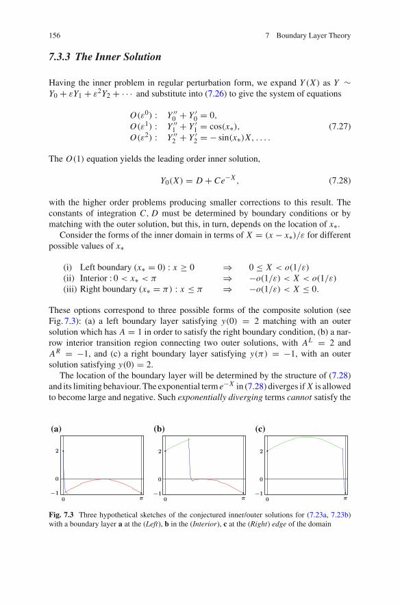
These options correspond to three possible forms of the composite solution (seeFig. 7.3): (a) a left boundary layer satisfying y(0) = 2 matching with an outersolution which has A = 1 in order to satisfy the right boundary condition, (b) a nar-row interior transition region connecting two outer solutions, with AL = 2 andAR = −1, and (c) a right boundary layer satisfying y(π) = −1, with an outersolution satisfying y(0) = 2.

The location of the boundary layer will be determined by the structure of (7.28)and its limiting behaviour. The exponential term e−X in (7.28) diverges if X is allowedto become large and negative. Such exponentially diverging terms cannot satisfy the

(a) (b) (c)

Fig. 7.3 Three hypothetical sketches of the conjectured inner/outer solutions for (7.23a, 7.23b)with a boundary layer a at the (Left), b in the (Interior), c at the (Right) edge of the domain

7.3 Constructing Boundary Layer Solutions 157

asymptotic matching condition (7.13) (with X → −∞ being the appropriate formof the ‘outer limit’ process) and are un-matchable.

Consequently options (ii) and (iii) are not feasible, and we conclude that theboundary layer must be at x∗ = 0 with the left boundary condition from (7.23b)being relevant, namely Y (0) = 2. Applying this condition reduces (7.28) to

Y0(X) = 2 + C(e−X − 1), (7.29)

where C remains to be determined.

7.3.4 Asymptotic Matching

Having identified the position of the boundary layer as x∗ = 0, we have the leadingorder inner solution (7.29), valid on 0 ≤ x < O(ε), and the outer solution (7.24),valid on 0 < x ≤ π . Since the right boundary lies in the outer domain, that boundarycondition determines A = −1 in (7.24), leaving C from (7.29) as the last remainingunknown.

Applying the matching condition (7.13) for Y0(X → ∞) and y0(x → 0) yields

limX→∞ 2 + C(e−X − 1) = 2 − C = lim

x→0sin(x) − 1 = −1 (7.30)

and hence C = 3.

7.3.5 The Composite Solution

The overlap shared in common by the leading order inner and outer solutions aboveis −1. Therefore we can form the boundary layer correction as

YBLC = Y0 − (−1) = 3e−X .

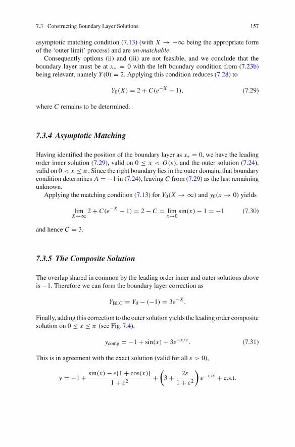
Finally, adding this correction to the outer solution yields the leading order compositesolution on 0 ≤ x ≤ π (see Fig. 7.4),

ycomp = −1 + sin(x) + 3e−x/ε. (7.31)

This is in agreement with the exact solution (valid for all ε > 0),

y = −1 + sin(x) − ε[1 + cos(x)]1 + ε2

+(3 + 2ε

1 + ε2

)e−x/ε + e.s.t.

158 7 Boundary Layer Theory

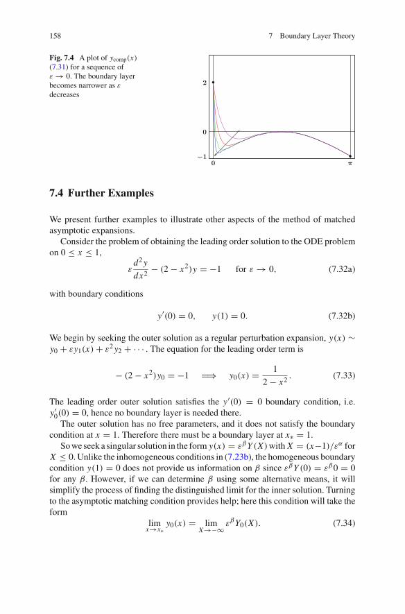
Fig. 7.4 A plot of ycomp(x)

(7.31) for a sequence ofε → 0. The boundary layerbecomes narrower as ε

decreases

7.4 Further Examples

We present further examples to illustrate other aspects of the method of matchedasymptotic expansions.

Consider the problem of obtaining the leading order solution to the ODE problemon 0 ≤ x ≤ 1,

εd2y

dx2− (2 − x2)y = −1 for ε → 0, (7.32a)

with boundary conditions

y′(0) = 0, y(1) = 0. (7.32b)

We begin by seeking the outer solution as a regular perturbation expansion, y(x) ∼y0 + εy1(x) + ε2y2 + · · · . The equation for the leading order term is

− (2 − x2)y0 = −1 =⇒ y0(x) = 1

2 − x2. (7.33)

The leading order outer solution satisfies the y′(0) = 0 boundary condition, i.e.y′0(0) = 0, hence no boundary layer is needed there.The outer solution has no free parameters, and it does not satisfy the boundary

condition at x = 1. Therefore there must be a boundary layer at x∗ = 1.Sowe seek a singular solution in the form y(x) = εβY (X)with X = (x−1)/εα for

X ≤ 0. Unlike the inhomogeneous conditions in (7.23b), the homogeneous boundarycondition y(1) = 0 does not provide us information on β since εβY (0) = εβ0 = 0for any β. However, if we can determine β using some alternative means, it willsimplify the process of finding the distinguished limit for the inner solution. Turningto the asymptotic matching condition provides help; here this condition will take theform

limx→x∗

y0(x) = limX→−∞ εβY0(X). (7.34)

7.4 Further Examples 159

While we have not determined Y0(X), it is assumed to be O(1), and for x → 1, wehave y0(1) = 1. Since the limit of the outer solution is O(1), so must be the limit ofthe inner solution, hence β = 0.

Substituting y(x) = Y (X) and x = 1 + εα X into (7.32a) yields

ε1−2αY ′′ − (2 − (1 + εα X)2)Y = −1

and in final form:

ε1−2αY ′′︸ ︷︷ ︸(1)

− (1 − 2εα X − ε2α X2)Y︸ ︷︷ ︸(2)

= −1︸︷︷︸(3)

. (7.35)

On a finite domain, α ≥ 0 with α > 0 describing boundary layers that narrow likeO(εα) as ε → 0. We note that for α > 0 the sum of terms in the parentheses in term(2) have leading order term (2 − x2) ∼ 1, so the higher order terms there cannotcontribute to a consistent dominant balance.

Balancing (2, 3) yields the distinguished limit for the outer solution, α = 0,with term (1) being sub-dominant, O(ε) � O(1). The other distinguished limit isα = 1/2, which balances all three terms at O(1).

We now have the form of the inner problem as

Y ′′ − (1 − 2ε1/2X − εX2)Y = −1, Y (0) = 0, (7.36)

for X ≤ 0. The presence of the ε1/2 suggests the expansion of the solution shouldtake the form Y (X) ∼ Y0 + ε1/2Y1 + εY2 + · · · . The leading order ODE is

Y ′′0 − Y0 = −1, (7.37)

with solutionY0(X) = Ae−X + BeX + 1. (7.38)

For this solution to be matchable to the outer solution as X → −∞, we must takeA = 0. Applying the boundary condition, Y0(0) = B + 1 = 0 then gives us thesolution,

Y0(X) = 1 − eX . (7.39)

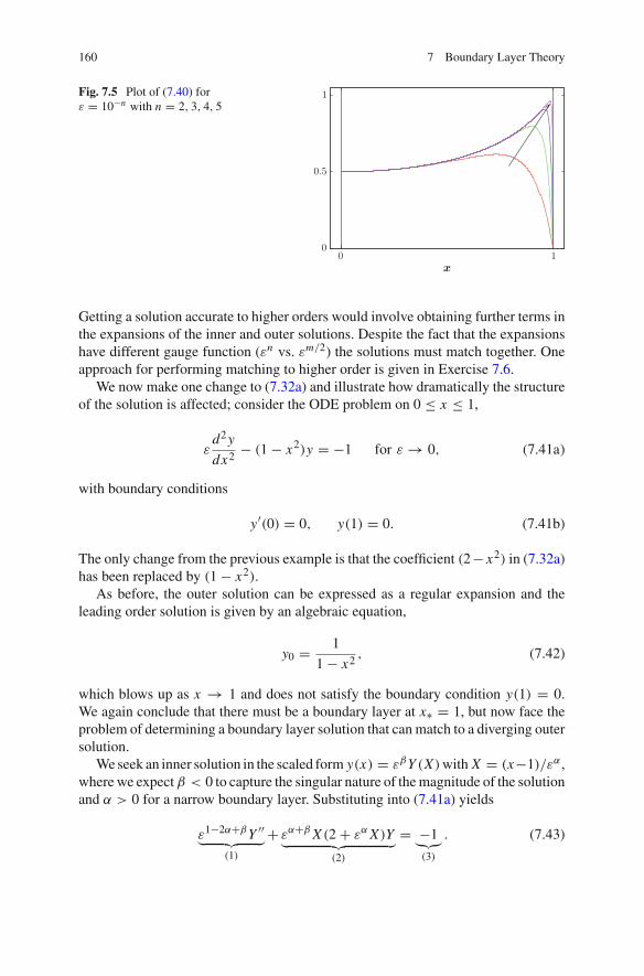
Since neither the leading order inner or outer solutions have any undetermined con-stants they should match automatically. This is indeed the case, and (7.34) appliedto (7.33) and (7.39) shows they match with an overlap limit of 1. Hence we canconstruct the leading order composite solution (see Fig. 7.5)

ycomp ∼ 1

2 − x2− e(x−1)/

√ε. (7.40)

160 7 Boundary Layer Theory

Fig. 7.5 Plot of (7.40) forε = 10−n with n = 2, 3, 4, 5

Getting a solution accurate to higher orders would involve obtaining further terms inthe expansions of the inner and outer solutions. Despite the fact that the expansionshave different gauge function (εn vs. εm/2) the solutions must match together. Oneapproach for performing matching to higher order is given in Exercise 7.6.

We now make one change to (7.32a) and illustrate how dramatically the structureof the solution is affected; consider the ODE problem on 0 ≤ x ≤ 1,

εd2y

dx2− (1 − x2)y = −1 for ε → 0, (7.41a)

with boundary conditions

y′(0) = 0, y(1) = 0. (7.41b)

The only change from the previous example is that the coefficient (2− x2) in (7.32a)has been replaced by (1 − x2).

As before, the outer solution can be expressed as a regular expansion and theleading order solution is given by an algebraic equation,

y0 = 1

1 − x2, (7.42)

which blows up as x → 1 and does not satisfy the boundary condition y(1) = 0.We again conclude that there must be a boundary layer at x∗ = 1, but now face theproblem of determining a boundary layer solution that can match to a diverging outersolution.

We seek an inner solution in the scaled form y(x) = εβY (X)with X = (x−1)/εα ,wherewe expect β < 0 to capture the singular nature of themagnitude of the solutionand α > 0 for a narrow boundary layer. Substituting into (7.41a) yields

ε1−2α+βY ′′︸ ︷︷ ︸(1)

+ εα+β X (2 + εα X)Y︸ ︷︷ ︸(2)

= −1︸︷︷︸(3)

. (7.43)

7.4 Further Examples 161

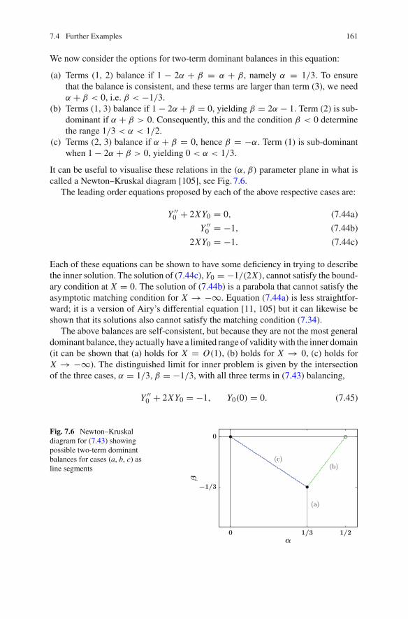
We now consider the options for two-term dominant balances in this equation:

(a) Terms (1, 2) balance if 1 − 2α + β = α + β, namely α = 1/3. To ensurethat the balance is consistent, and these terms are larger than term (3), we needα + β < 0, i.e. β < −1/3.

(b) Terms (1, 3) balance if 1 − 2α + β = 0, yielding β = 2α − 1. Term (2) is sub-dominant if α + β > 0. Consequently, this and the condition β < 0 determinethe range 1/3 < α < 1/2.

(c) Terms (2, 3) balance if α + β = 0, hence β = −α. Term (1) is sub-dominantwhen 1 − 2α + β > 0, yielding 0 < α < 1/3.

It can be useful to visualise these relations in the (α, β) parameter plane in what iscalled a Newton–Kruskal diagram [105], see Fig. 7.6.

The leading order equations proposed by each of the above respective cases are:

Y ′′0 + 2XY0 = 0, (7.44a)

Y ′′0 = −1, (7.44b)

2XY0 = −1. (7.44c)

Each of these equations can be shown to have some deficiency in trying to describethe inner solution. The solution of (7.44c), Y0 = −1/(2X), cannot satisfy the bound-ary condition at X = 0. The solution of (7.44b) is a parabola that cannot satisfy theasymptotic matching condition for X → −∞. Equation (7.44a) is less straightfor-ward; it is a version of Airy’s differential equation [11, 105] but it can likewise beshown that its solutions also cannot satisfy the matching condition (7.34).

The above balances are self-consistent, but because they are not the most generaldominant balance, they actually have a limited range of validitywith the inner domain(it can be shown that (a) holds for X = O(1), (b) holds for X → 0, (c) holds forX → −∞). The distinguished limit for inner problem is given by the intersectionof the three cases, α = 1/3, β = −1/3, with all three terms in (7.43) balancing,

Y ′′0 + 2XY0 = −1, Y0(0) = 0. (7.45)

Fig. 7.6 Newton–Kruskaldiagram for (7.43) showingpossible two-term dominantbalances for cases (a, b, c) asline segments

162 7 Boundary Layer Theory

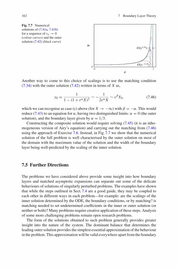
Fig. 7.7 Numericalsolutions of (7.41a, 7.41b)for a sequence of εn → 0(colour curves) and the outersolution (7.42) (black curve)

Another way to come to this choice of scalings is to use the matching condition(7.34) with the outer solution (7.42) written in terms of X as,

y0 = 1

1 − (1 + εα X)2∼ − 1

2εα X∼ εβY0, (7.46)

which we can recognise as case (c) above (for X → −∞) with β = −α. This wouldreduce (7.43) to an equation for α, having two distinguished limits: α = 0 (the outersolution), and the boundary layer given by α = 1/3.

Constructing the composite solution would require solving (7.45) (it is an inho-mogeneous version of Airy’s equation) and carrying out the matching from (7.46)using the approach of Exercise 7.6. Instead, in Fig. 7.7 we show that the numericalsolution of the full problem is well characterised by the outer solution on most ofthe domain with the maximum value of the solution and the width of the boundarylayer being well-predicted by the scaling of the inner solution.

7.5 Further Directions

The problems we have considered above provide some insight into how boundarylayers and matched asymptotic expansions can separate out some of the delicatebehaviours of solutions of singularly perturbed problems. The examples have shownthat while the steps outlined in Sect. 7.4 are a good guide, they may be coupled toeach other in different ways in each problem—for example: are the scalings of theinner solution determined by the ODE, the boundary conditions, or by matching? ismatching needed to set undetermined coefficients in the inner or outer solution (orneither or both)?Many problems require creative application of these steps. Analysisof some more challenging problems remain open research problems.

The form of the solutions obtained to such problem generally provides greaterinsight into the nature of the system. The dominant balance that determines theleading outer solution provides the simplest essential approximation of the behaviourin the problem. This approximationwill be valid everywhere apart from the boundary

7.5 Further Directions 163

layers. Matched asymptotics provides understanding of whether the boundary layersare necessary to pin-down properties of the outer solution or merely correct thesolution in narrow regions. Often, knowledge of the physical system being modelledcan guide expectations on boundary layer positions and dominant balances; this cansometimes simplify the mathematical steps. Sometimes, the matched asymptoticswill uncover unexpected dominant balances that can highlight novel and importantbehaviours in the problem.

This chapter only hints at the broad array of models that can be studied usingmatched asymptotics and the types of behaviours that can result. Some of theseinclude boundary layers within boundary layers (nested layers or “triple decks”),boundary layers that begin at higher orders (“corner layers”), and problems withunusual gauge functions. There is a wide array of books that give further studies ofboundary layer problems [47, 48, 58, 78, 92] and some primary sources on the theoryof asymptotic matching are [60, 101].

7.6 Exercises

7.1 Evaluate limε→0 e−1/ε/εn to demonstrate that exponentially small terms aresmaller than all algebraic terms.

7.2 Determine the three possible dominant balances for (7.25) that could occur forx∗ = π/2, noting that cos(x) → 0 as x → x∗.

7.3 Consider the problem for y(x) on 0 ≤ x ≤ 1 with ε → 0,

εd2y

dx2− (4 − x2)y = cos

(π2 x

)y(0) = −1 y(1) = 2

(a) Determine the two distinguished limits for this problem.(b) Write the leading order outer solution y0(x).(c) Find the leading order inner solutions Y0(X).(d) Write the leading order uniformly-valid solution.

7.4 Consider the initial value problem for y(x) on 0 ≤ x for ε → 0,

εd2y

dx2+ 2

dy

dx− 6y = 5x, y(0) = 0, y′(0) = 4

ε2.

You are given that the solution has a boundary layer at x∗ = 0.

(a) Determine the leading order inner solution.(b) Write the outer limit of the inner solution to determine a necessary matching

condition on the outer solution.(c) Determine the leading order outer solution for x > 0.

164 7 Boundary Layer Theory

7.5 Consider the problem for y(x) on 0 ≤ x ≤ 1 with ε → 0,

εd2y

dx2+ 2

dy

dx+ ey = 0, y(0) = 0, y(1) = 0.

(a) Find the general leading order outer solution y0(x).(b) Find the leading order inner solution Y0(X) and determine where the boundary

layer occurs.(c) Write the leading order composite solution.(d) Determine the next term in the outer solution, y1(x).

7.6 Consider the problem for y(x) on 0 ≤ x ≤ 1 with ε → 0,

εd2y

dx2− dy

dx+ y = 2x, y(0) = −2, y(1) = 1.

(a) Determine the distinguished limit for the inner problem for this equation. Bysolving the leading order inner problem, determine where the boundary layeroccurs.

(b) Obtain the first two terms in the expansion of the inner solution (with the appro-priate boundary conditions imposed),

Y (X) ∼ Y0(X) + εY1(X).

(c) Determine the first two terms in the expansion of the outer solution (with theappropriate boundary conditions imposed),

y(x) ∼ y0(x) + εy1(x).

(d) The inner solution will have undetermined constants. These constants can bedetermined using higher-order matching using intermediate variables [60, 101]via the following steps:

(i) Analogous to (7.12), define small parameter η with εα � η � 1.(ii) Define the intermediate variable x̂ as x̂ = (x − x∗)/η.(iii) Use the relations

x = x∗ + ηx̂, X = η

εαx̂

to write the outer and inner solutions both in terms of the intermediatevariable x̂ and ε, η.

(iv) Use the relations εα � η � 1 to expand out exponential functions oreliminate small terms in the solutions on the overlap region, with x̂ = O(1).

(v) Arrange the remaining terms as an ordered asymptotic expansion involvingη, ε and determine the remaining constants through matching of terms.

(e) Write the uniform solution valid up through O(ε) terms.

7.6 Exercises 165

7.7 Consider the problem for y(x) on 0 ≤ x ≤ 2 with ε → 0,

x2 + y2 = 4 − εdy

dx, y(0) = 3

ε.

(a) Determine the first two terms in the outer solution,y ∼ y0 + εy1.

(b) Boundary layers can occur at x∗ = 0 and x∗ = 2. For each case, determinethe α, β for each distinguished limit and write its corresponding leading orderequation for Y0(X). Note that there are two singular distinguished limits atx∗ = 0.

7.8 Consider the problem for y(x) on 0 ≤ x ≤ 1 for ε → 0,

εd2y

dx2− y = −4 + ε2y

(x − 1)3, y(0) = 0, y(1) = 0.

The leading order outer solution is y0(x) ≡ 4.

(a) Determine the leading order inner solution for the boundary layer at x∗ = 0.(b) At x∗ = 1, there are two different distinguished limits. Determine α for each

and obtain the respective leading order equations for each Y0(X).Since these solutions have different α’s, one layer is nested inside the other. The“inner-inner” layer solution should satisfy boundary condition at x = 1. The(wider) “intermediate inner” layer should asymptotically match to the outer andinner-inner solutions for the limits X → −∞ and X → 0 respectively in thistriple deck problem.