Chapter 6 Transmission Lines - University of...
60
6-1 Chapter 6 Transmission Lines ECE 3317 Dr. Stuart A. Long
Transcript of Chapter 6 Transmission Lines - University of...

6-1
Chapter 6 Transmission Lines
ECE 3317Dr. Stuart A. Long

6-2

6-3
0
0
1
2
Voltage ( )
Current ( c
V( )
los
I( ) e d)
t
C
tC
z d
z d
C z
C
α
α
= •
=
⊥
•
∫
∫
E
H
s
s
p.133
( )a
( )b
General Definitions
http://www.cartoonstock.com

6-4
* *
0
Power
Characteristic infinite line with Impedance
1 1 ˆRe V( ) I ( ) Re 2 2
V( ) Z with I )
(
A
z z dA
zz
= × •
=
∫ E H z
no reflection
( )c
p.133
General Definitions
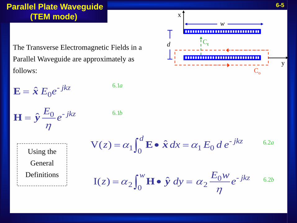
6-5Parallel Plate Waveguide (TEM mode)
-0
-0
-1 1 00
-02 20
ˆ
ˆ
ˆ V( )
ˆ I( )
jkz
jkz
d jkz
w jkz
E e
E e
z dx E d e
E wz dy e
η
α α
α αη
=
=
= • =
= • =
∫
∫
E
H
E
H
x
y
x
y
x
Co
w
d
y
Ct
6.1a
6.1b
6.2a
6.2b
The Transverse Electromagnetic Fields in a Parallel Waveguide are approximately as follows:
Using the General
Definitions
6-6
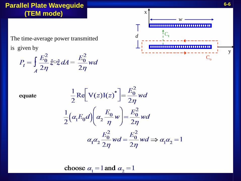
The time-average power transmitted is given by
x
Co
w
d
y
Ct
Parallel Plate Waveguide (TEM mode)

6-7
0
0
0 [ ]
V( )
I( )
Z
jkz
jkz
z E de
E wz e
dw
η
η
−
−
Ω
=
=
=
6.3a
6.3b
6.4
x
Co
w
d
y
Ct
Parallel Plate Waveguide (TEM mode)

6-8Coaxial Line
The fields inside a coaxial line for the TEM mode are given by
6.5a
6.5b
Using the General
Definitions
6.6a
6.6b
Co
ab
Ct
6-9
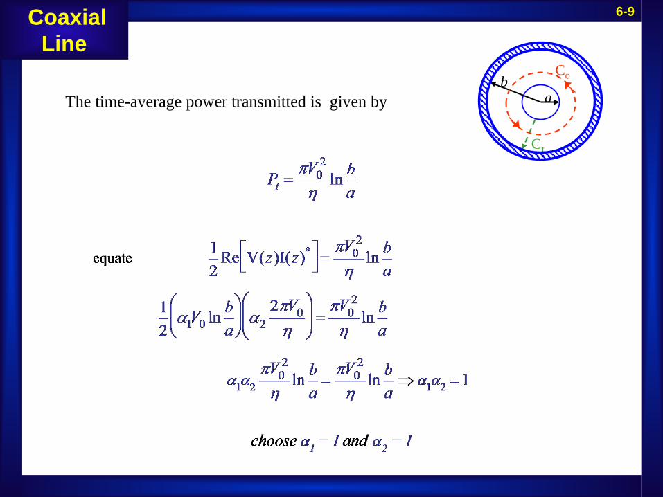
The time-average power transmitted is given by
Co
ab
Ct
Coaxial Line
6-10
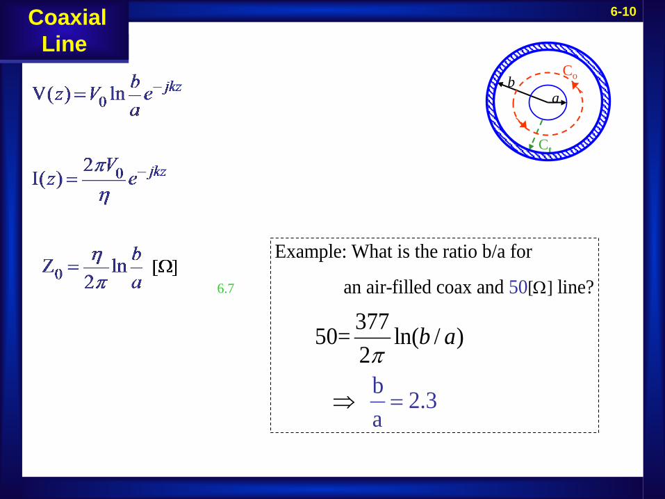
Coaxial Line
[ ]
Example: What is the ratio b/a for
an air-filled 50coax and line?
37750= ln( /2
b .3a
)
2
b aπ
Ω
=⇒
6.7
Coaxial Line
Co
ab
Ct

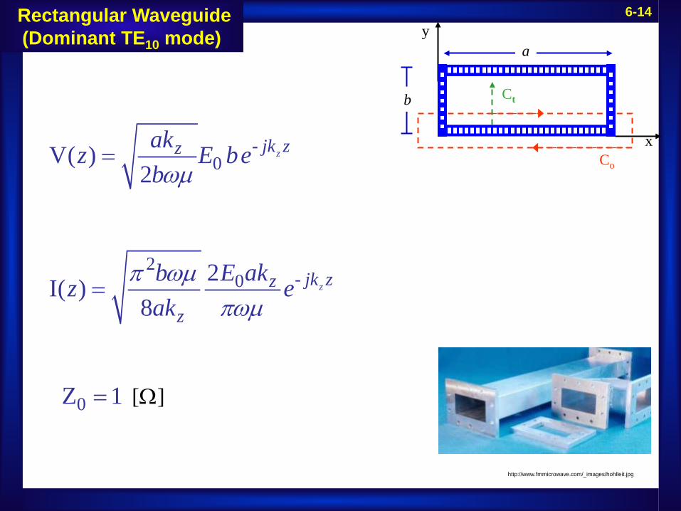
6-11Rectangular Waveguide (Dominant TE10 mode)
xCo
a
b
y
CtThe Electromagnetic fields in a Rectangular
Waveguide for the are TE10 mode are
6.8a
6.8b
6.8c
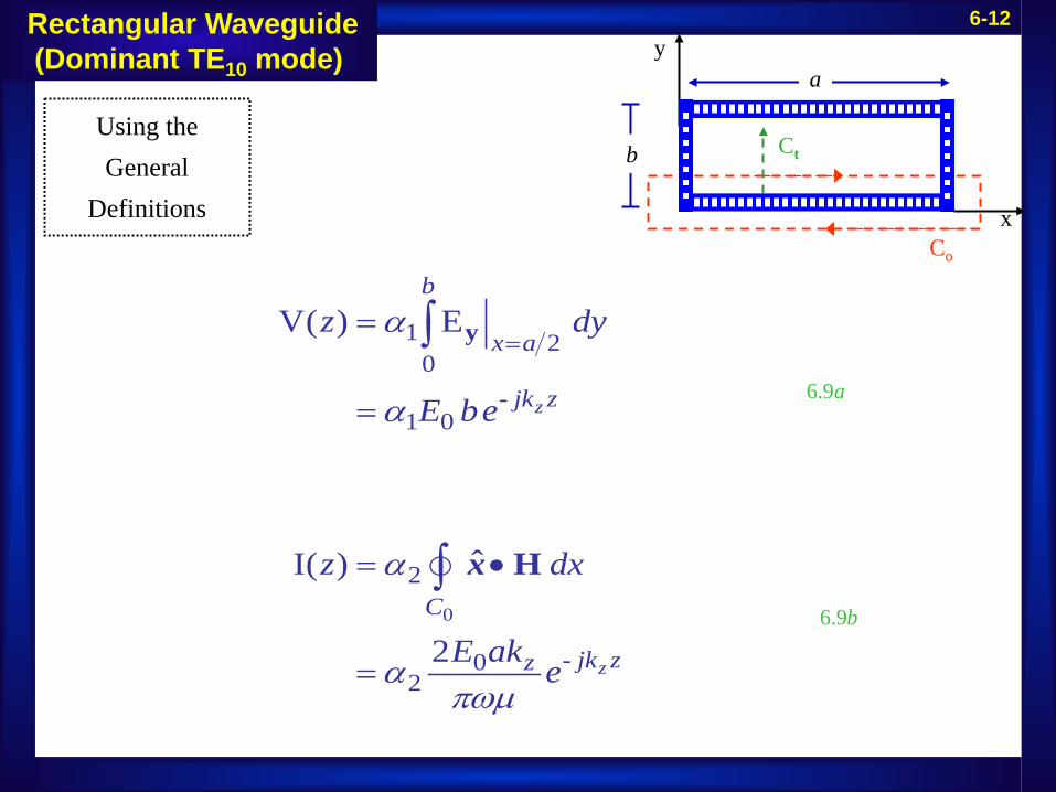
6-12Rectangular Waveguide (Dominant TE10 mode)
0
1 20
-1 0
2
-02
V( ) E
ˆ I( )
2
z
z
b
x a
jk z
C
jk zz
z dy
E be
z dx
E ak e
α
α
α
απωµ
==
=
= •
=
∫
∫
y
H
x
xCo
a
b
y
CtUsing the General
Definitions
6.9a
6.9b
6-13
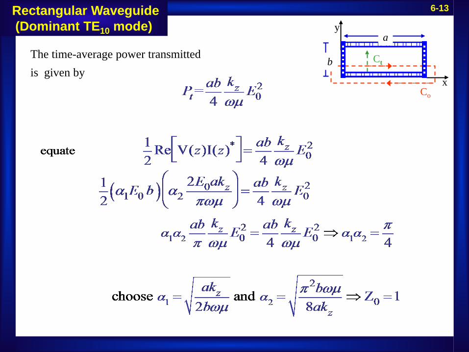
The time-average power transmitted is given by
xCo
a
b
y
Ct
Rectangular Waveguide (Dominant TE10 mode)
6-14
-0
2-0
0 [ ]
V( )2
2I( )8
Z 1
z
z
jk zz
jk zz
z
akz E beb
E akbz eak
ωµ
π ωµπωµ
Ω
=
=
=
xCo
a
b
y
Ct
Rectangular Waveguide (Dominant TE10 mode)
http://www.fmmicrowave.com/_images/hohlleit.jpg
6-15
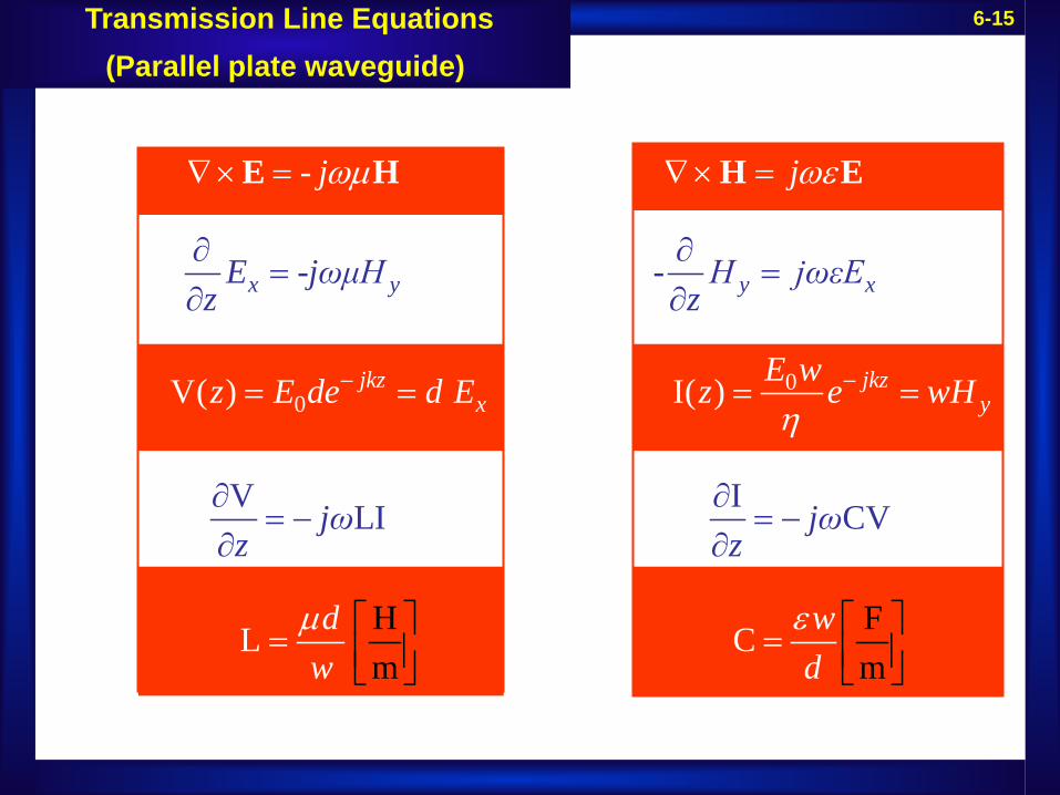
00
-
V LI
-
V( ) ( )
Ijkz jkzx y
x y y xE -jωμH H jω
j j
E wz E de d E z e
εEz z
j
w
ω
H
z
ωµ ωε
η− −
∇× = ∇× =
= = = =
∂ ∂= =
∂ ∂
∂= −
∂
E H H E
I CV
L H F m
C m
d ww
jωz
dµ ε
= =
= −∂
∂
Transmission Line Equations (Parallel plate waveguide)

6-16
22
2
+ -
+ -0
0
wave equationV LCV 0
V V V
1I V VZ
LC
LZC
-jkz jkz
-jkz jkz
z
e e
e e
k
ω
ω
+
+
∂+ =
∂
= +
= −
=
= 6.18
6.16
6.17
6.15
Transmission Line Equations (Parallel plate waveguide)
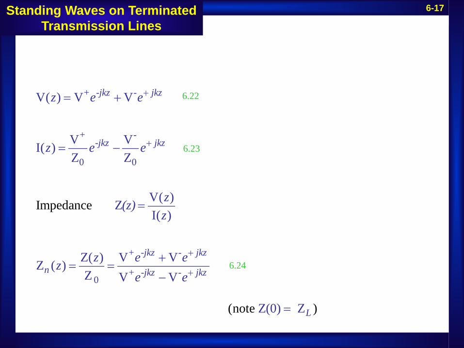
6-17Standing Waves on Terminated Transmission Lines
+ -
+ -
0 0
+ -
+ -0
V( ) V V
V VI( )Z Z
V( ) ZI( )
Z( ) V VZ ( )Z V V
Impedan
Z(0) Z
ce
(note )
-jkz jkz
-jkz jkz
-jkz jkz
n -jkz jkz
L
z e e
z e e
z(z)z
z e eze e
+
+
+
+
= +
= −
=
+= =
−
=
6.22
6.23
6.24
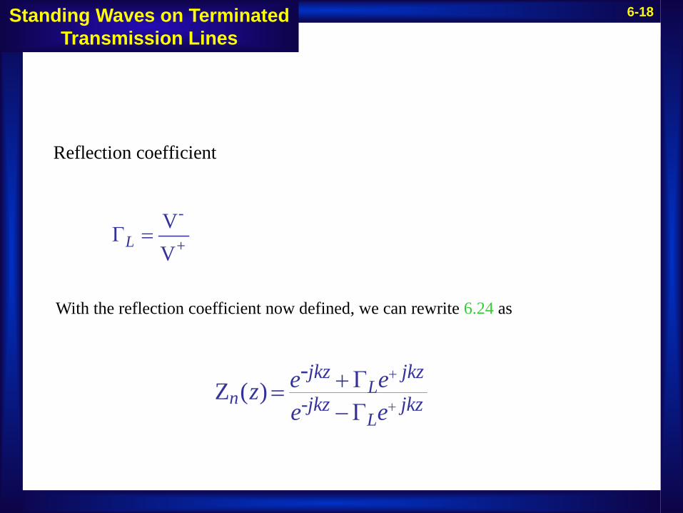
6-18
-
+
Reflection coefficient
ΓV
V L =
ΓZ ( )Γ
LnL
jkz jkz-jkz jkz-e ez
e e
+
+
+=−
With the reflection coefficient now defined, we can rewrite 6.24 as
Standing Waves on Terminated Transmission Lines

6-19
GZLZ
Transmission LineGenerator Load
GV
6.27
Evaluating at the Load (Z 0)
Z 11Z( or0)Z ( 0) Z 1 Z 10
zn
LL
L L
z nznL Ln
=
−+ Γ==
= Γ =− +
=Γ
Evaluating at a point along line ( )Z
Z Z tanZ( ) 0Z ( )Z Z Z tan0 0
z ln
j klz l Lz ln j klL
= −
+= −= − = =
+
6.25
Standing Waves on Terminated Transmission Lines
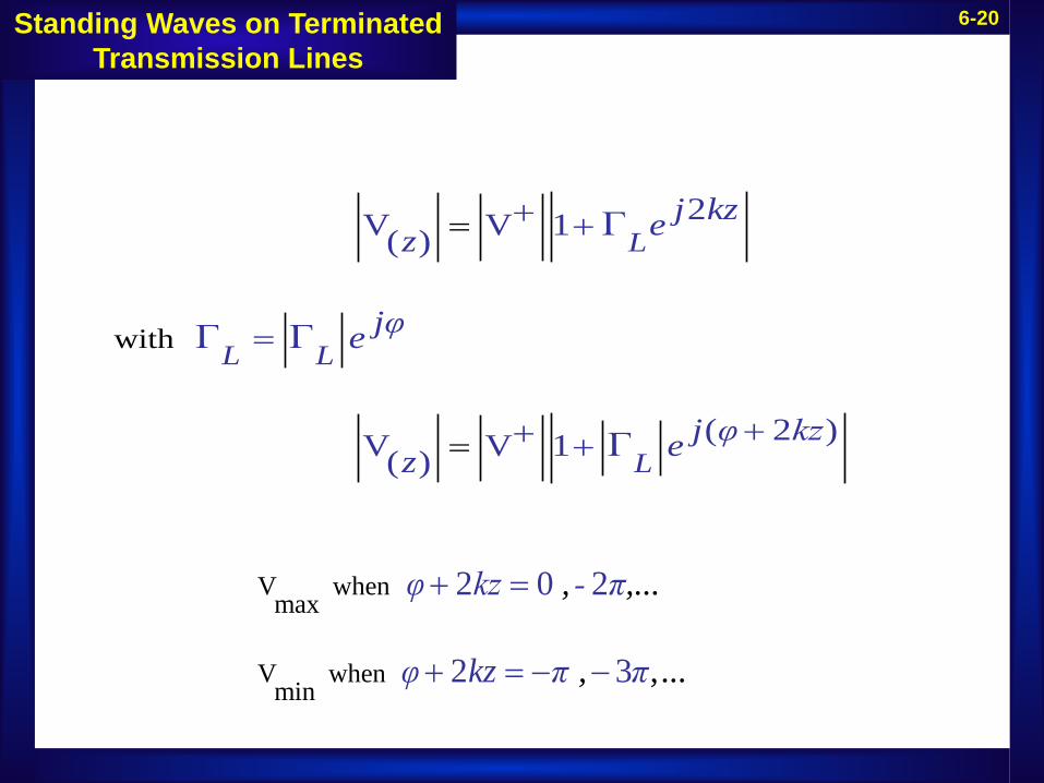
6-20
V whenmax
V when min
2 0 2
2 3
,
φ kz - π
φ
, ,...
, ..kz π π .
+ =
+ = − −
with
2 V V 1( )
( 2 )V V
1( )
Γ
Γ Γ
Γ
L
L L
L
j kzez
jφe
j φ kzez
+ +
++
=
=
+=
Standing Waves on Terminated Transmission Lines

6-21Standing Wave Pattern
z
1+ LΓ
1
1- LΓ
+
V( )V
z
( 2 )V V 1( )
V( ) ( 2 )1V
Γ
Γ
L
L
j φ kzez
z j φ kze
++ +
++
=
=+
Fig. 6.6

6-22Crank Diagram
( 2 )1 ΓLj φ kze ++
Im
Re1ΓL
Fig. 6.6
( 2 )V V 1( )
V( ) ( 2 )1V
Γ
Γ
L
L
j φ kzez
z j φ kze
+
+
= +
+=
+
+
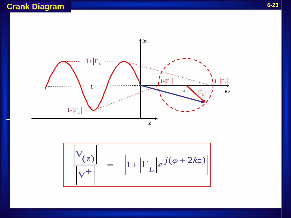
6-23
1- LΓ
Im
Re1 ΓL
V( ) ( 2 )1V
ΓLz j φ kze +++
=
1- LΓ 1+ LΓ
1+ LΓ
1
z
Crank Diagram
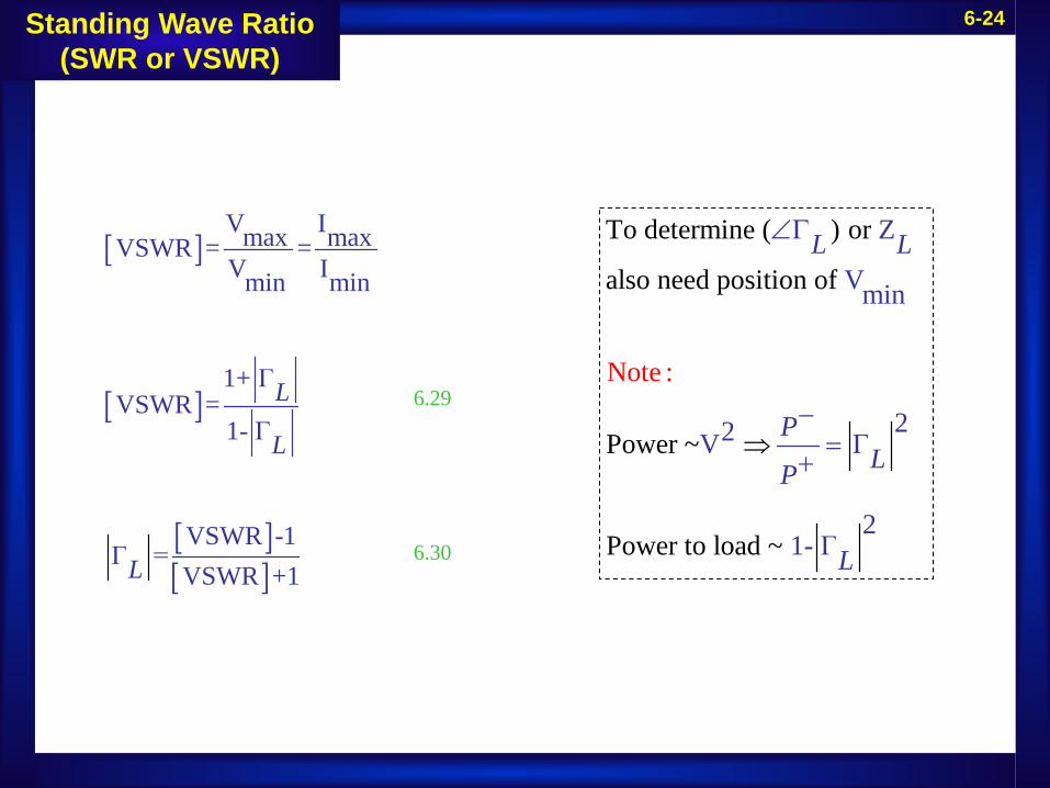
6-24
[ ]
[ ]
[ ][ ]
V Imax maxVSWR = =V Imin min
1+ ΓVSWR =
1- Γ
VSWR -1Γ =
VSWR +1
L
L
L
6.29
Z
Vmin
N
To dete
ote :
rmine ( ) or
also need position of
P2
ower ~
Power t
2V Γ
21o load ~ Γ
-
L L
PLP
L
⇒
∠Γ
−=
+
6.30
Standing Wave Ratio (SWR or VSWR)

6-25
[ ] [ ]Z 17.4 30 Z 500
Z 1 Z 0Γ 0.24 .55Z 1 Z 0
1.
an
99Γ 0
d
.6
or
jL
ZnL L jL ZnL L
jeL
= − =
− −= = = − −
+ +
−=
Ω Ω
Example
ZLZ0
+V 5. V25 =Ex. 6.6
Γ 0.6
Γ 1.99
L
Lφ
=
= ∠ =V when
max
V when min
2 0 2
2 3
,
φ kz - π
φ
, ,...
, ..kz π π .
+ =
+ = − −
where
z
1
+
V(z)V
1.6
0.4
-0.092λ-0.342λ-0.592λ

6-26
V 2min
( 1.99)
where
.0922 2(2 )
m
m
k z
zk
φ π
π φ π λ λπ
+ = −
− − − += = = −
z
8.4
2.1
-0.092λ-0.342λ-0.592λ
V
maxV
minV
Ex. 6.6
Example
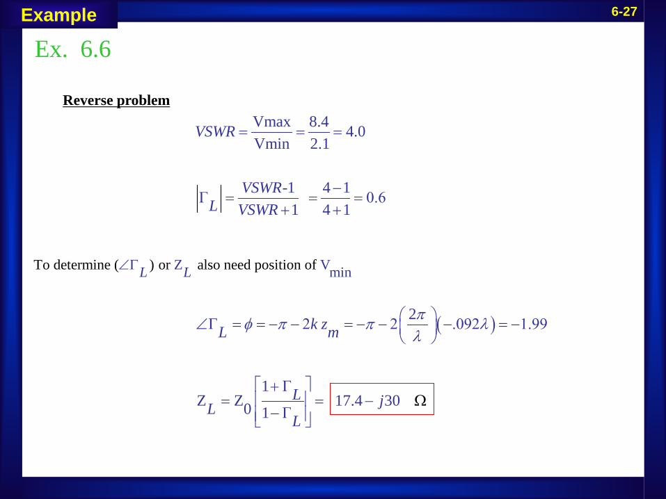
6-27
( )
Vmax 8.4 4.0Vmin 2.1
-1 4 1Γ 0.61 4 1
2Γ 2 2 .092 1.99
1 ΓZ Z 17.4 300 1 Γ
VSWR
VSWRL VSWR
k zL m
L jLL
πφ π π λλ
= = =
−= = =
+ +
∠ = = − − = − − − = −
+ = = −−
Ω
Reverse problem
Ex. 6.6
To determine ( ) or also need position ofZ VminL L∠Γ
Example
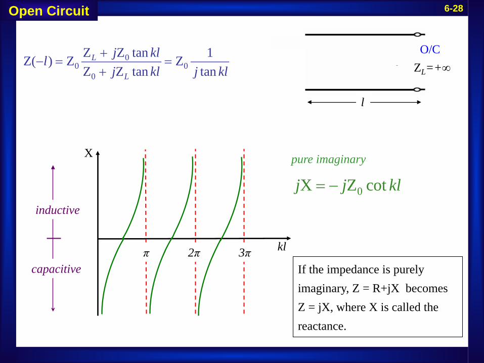
6-28Open Circuit
00 0
0
Z Z tan 1Z( ) Z Z Z Z tan tan
L
L
j kllj kl j kl
+− = =
+
X
klπ 2π 3π
inductive
capacitive
0X Z cotj j kl= −
pure imaginary
ZL=+∞O/C
l
If the impedance is purely imaginary, Z = R+jX becomes Z = jX, where X is called the reactance.

6-29
ZL=+∞O/C
l
X
klπ
inductive
capacitive
0X Z cotj j kl= −
pure imaginary
( )at
(short circuit)
2 4
Z 0 4 near is inductive
near is ca
Z
Note:
0 Z pa citi ve
kl l
kl
kl
π λ
λ
π
= ⇒ =
− =
≤
≥
Open Circuit
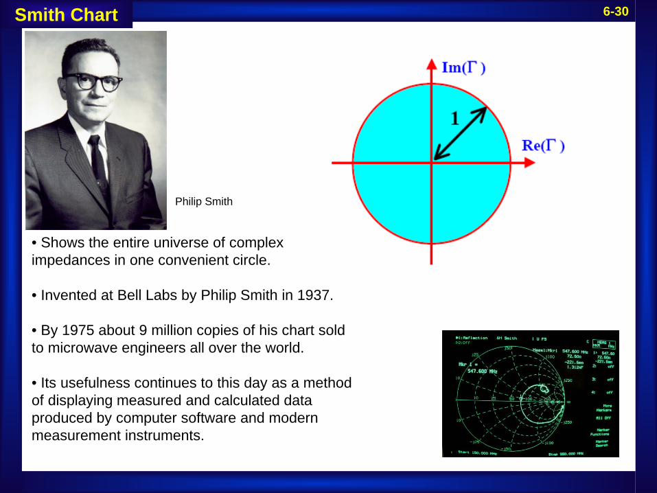
6-30Smith Chart
• Shows the entire universe of complex impedances in one convenient circle.
• Invented at Bell Labs by Philip Smith in 1937.
• By 1975 about 9 million copies of his chart sold to microwave engineers all over the world.
• Its usefulness continues to this day as a method of displaying measured and calculated data produced by computer software and modern measurement instruments.
Philip Smith
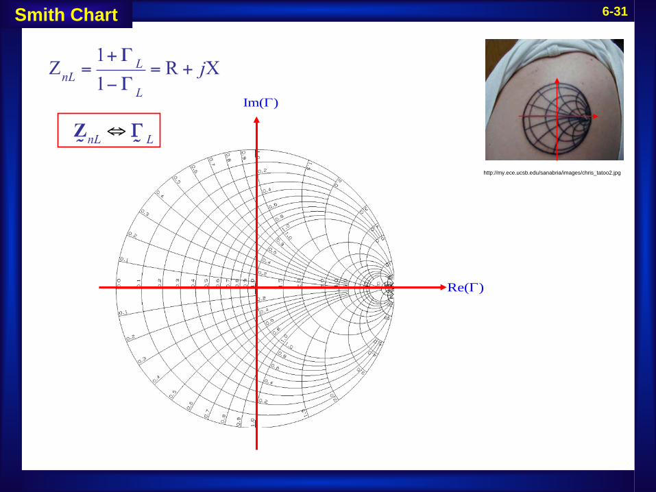
6-31
Im( )Γ
Re( )Γ
Smith Chart
http://my.ece.ucsb.edu/sanabria/images/chris_tatoo2.jpg

6-32Constant R Circles
on Chart
Rn=0Rn=0.5
Rn=1
Rn=2 Rn=50
Z Chart
Rn: normalized resistance
nnnL [ ]
mpedance =
resistance + reactance
X Z i
Rj
j Ω= +
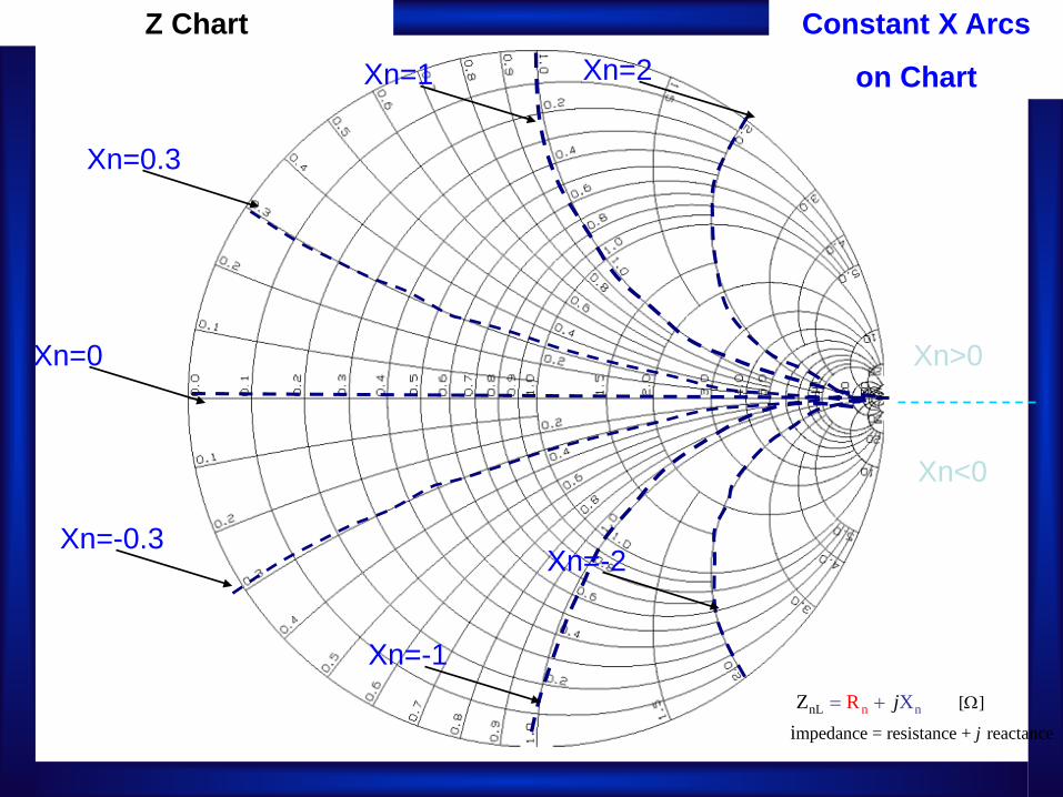
6-33
Xn=0
Xn=0.3
Xn=-0.3
Xn=1
Xn=-1
Xn=2
Xn=-2
Xn>0
Xn<0
Constant X Arcs
on Chart
Z Chart
nnnL [ ]
mpedance =
resistance + reactance
X Z i
Rj
j Ω= +

6-34nnnL
nL
[ ]
X R Z
[ ] 0.2 0.3 Z
j
j
Ω= +
Ω= −
Rn=0.2 circle
Xn=-0.3 arc x

6-35nnnL
nL
[ ]
X R Z
[ ] 0.2 0.3 Z
j
j
Ω= +
Ω= −
x
Using your compass draw the 0.2-j0.3 circle with center at zn=1.
(NOTE: this circle is not on the chart until you draw it.
1 Xcircle
j+
6-36
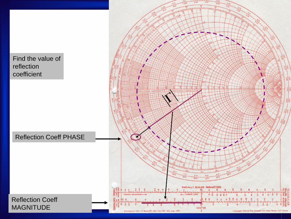
Find the value of reflection coefficient
Reflection Coeff magnitude Reflection Coeff magnitude Reflection Coeff MAGNITUDE
Reflection Coeff PHASE
6-37
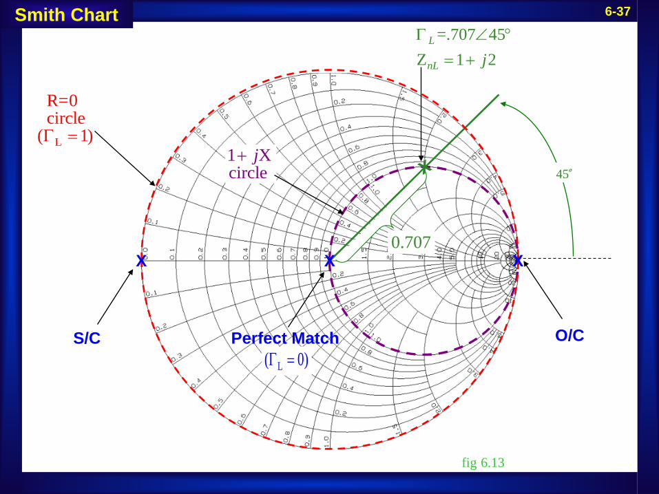
S/C O/CPerfect Match
1 Xcircle
j+
=.707 45Z 1 2
L
nL jΓ ∠ °
= +
45
L
R=0 circle( 1)Γ =
L( 0)Γ =
0.707XXX
fig 6.13
Smith Chart
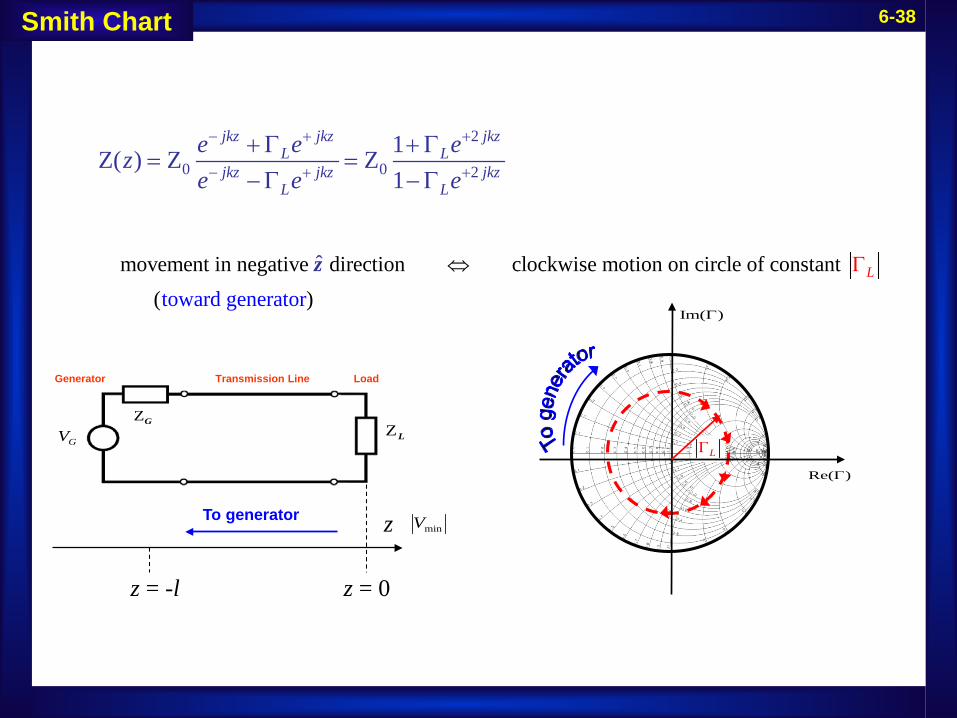
6-38
2
0 0 21Z( ) Z Z1
jkz jkz jkzL L
jkz jkz jkzL L
e e eze e e
− + +
− + +
+ Γ + Γ= =
−Γ −Γ
movement in negative direction clockwise motion on circle of constant toward generator
( )
ˆ LΓ⇔z
GZLZ
Transmission LineGenerator Load
GV
z
z = 0z = -l
minV
ΓL
Im( )Γ
Re( )Γ
To generator
Smith Chart

6-39
ΓL
Im( )Γ
Re( )Γ
360 =2 rad =2
1
complet
Y ( )= -Z
e circle ( )
can just replace by ( )
N
(
ote
)
:
n L Ln
zz
λπ
Γ⇒
°
Γ
V( ) 21V
ΓLz j kze= ++
Smith Chart
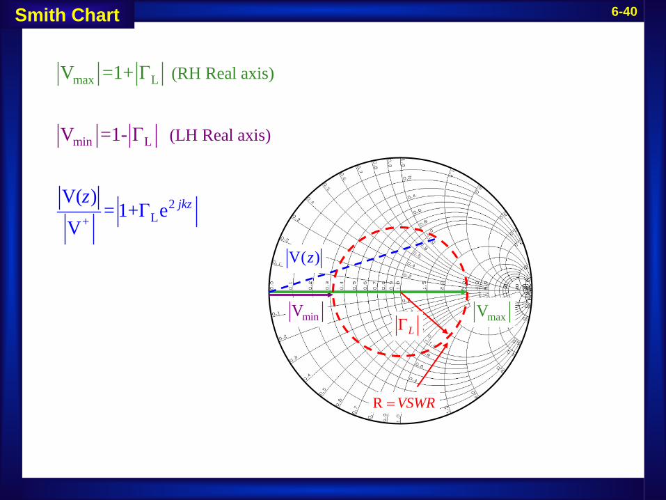
6-40
min L
ma
L+
L
2
x (RH Real axi
(LH Real axis)
s)
V =1- Γ
V( )= 1+Γ
V =1+ Γ
eV
jkzz
maxVminV
V( )z
ΓL
R VSWR=
Smith Chart

6-41
Z 1 2 nL j= +
minV maxVΓL
VLoad
nLZ
Smith Chart
=.707 45Γ ∠ °
max L
min LV =1
V =1+ Γ =1
- Γ
+0.707=1
1 .07
.7
0
0
2
7
7 0. 93= − =
VLoad
+
V(z)V
1.707
0.293
( )minz V ( )maxz Vz
45°

6-42
Z 1 2 nL j= +
Smith Chart
=.707 45Γ ∠ °
VLoad
+
V(z)V
1.707
0.293
( )minz V ( )maxz Vz
minV maxVΓL
VLoad
nLZ45°
360 on Smith Chart=2
180 on Smith Chart=4
4545 on Smith Chart=
3601
2 16
λ
λ
λ
°
°
° → =
4λ
16λ
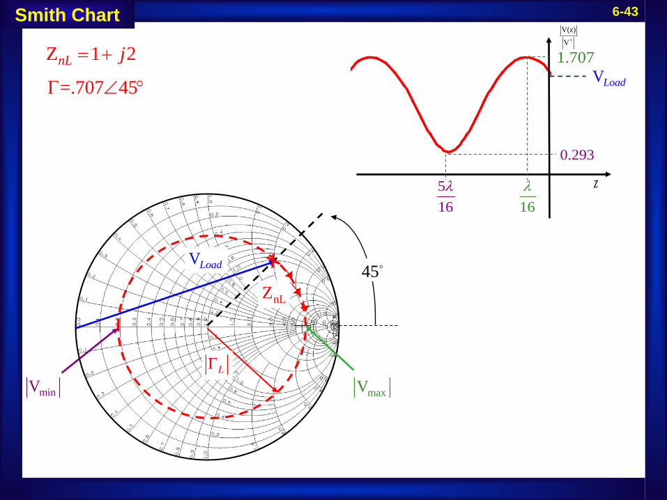
6-43
Z 1 2 nL j= +
minV maxVΓL
VLoad45
nLZ
+
V(z)V
1.707
0.293
VLoad
516λ
16λ z
Smith Chart
=.707 45Γ ∠ °
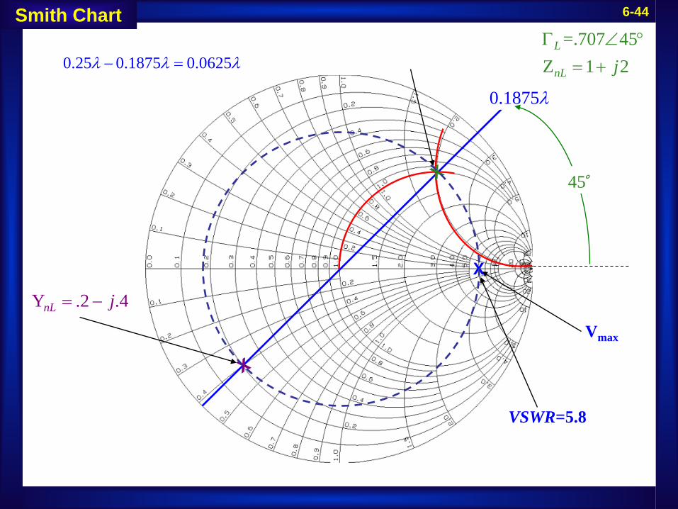
6-44
VSWR=5.8
X
0.1875λ
Y .2 .4 nL j= −
=.707 45Z 1 2
L
nL jΓ ∠ °
= +
45
Vmax
0.25 0.1875 0.0625λ λ λ− =
Smith Chart
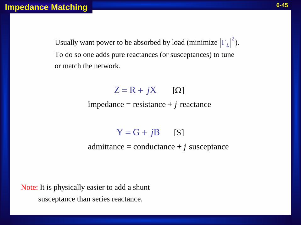
6-45Impedance Matching
2Usually want power to be absorbed by load (minimize ).To do so one adds pure reactances (or susceptances) to tune or match the network.
Γ
L
[ ]
mpedance = resistance + reactance
[S]
admittance = conductance + suscepta
nce
Z R X
Y
i
G B
j
j
j
j
Ω= +
= +
It is physically easier to add a shunt susceptance than series reactaNote:
nce.
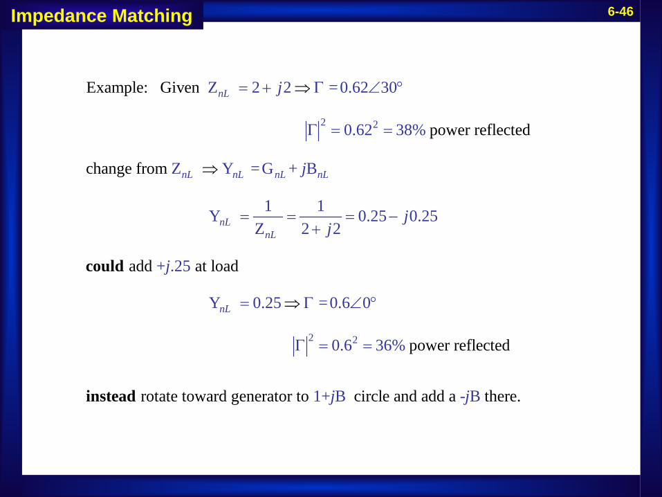
6-46
2 2
Z 2 2 =0.62 30
0.
Example: Given
power reflected
cha
62 38%
Z Y =G + B
1 1
nge from
Y 0.2Z 2 2
nL
nL nL nL nL
nLnL
j
j
j
= + Γ ∠ °
Γ = =
= = =+
⇒
⇒
2 2
5 0.25
+ .25
Y 0.25 =0.6 0
0.6 3
add at load
power reflected
rotate tow
6
ard generator
%
t 1+ Bo cir
nL
j
j
j
−
= Γ ∠ °
Γ = =
⇒
could
instead cle and add a tB .- herej
Impedance Matching

6-47Smith Chart
0S
.ol
36utio
20.21
n: Add at 1.57
1.Or - 57 at 9j
jλ
λ+
0.170. 0.2198041 λλ λ=+0.320. 0.3632041 λλ λ=+
Z 2 2 nL j= +
0.178λ
Y 0.25 0. 5 2nL j= −
1 1.57j+
1 1.57j−
0.322λ
0.041λ
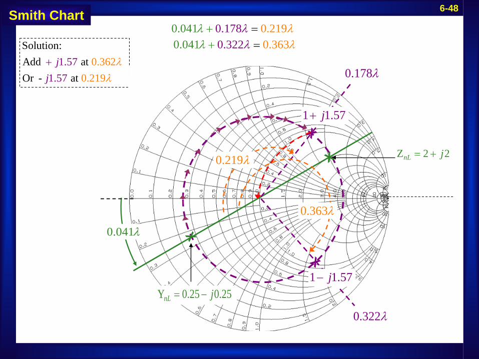
6-48Smith Chart
0S
.ol
36utio
20.21
n: Add at 1.57
1.Or - 57 at 9j
jλ
λ+
0.170. 0.2198041 λλ λ=+0.320. 0.3632041 λλ λ=+
Z 2 2 nL j= +
0.178λ
Y 0.25 0. 5 2nL j= −
1 1.57j+
1 1.57j−
0.322λ
0.363λ
0.219λ
0.041λ

6-49
http://www.ocf.berkeley.edu/~joydip/smithchart/index.html
Smith Chart Applet

6-50Standing Wave Pattern
ZL
z0.219λ− 0
nLZ
1.62
0.78
0.219λ
0.042λ1.55
( )
( )
max
min
1.55
1.620.38
0.78
0
0.219
loadV V
VV
V λ
=
=
=
=
=
−
Voltages: Unmatched Line
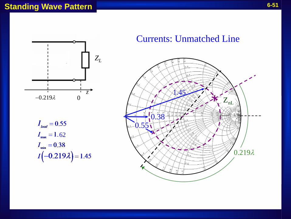
6-51Standing Wave Pattern
ZL
z0.219λ− 0
nLZ
0.219λ
0.550.38
62
1.45
Currents: Unmatched Line

6-52Standing Wave Pattern
ZL
z
-jB
0.219λ− 0nLZ
1.62
0.78
0.219λ
1.55
( )
max
min
1.551.620.38
0.780.219
loadVVV
V λ
=
=
=
=−
Voltages: Matched Line

6-53
ZL
z0
ZL
z
-jB
0.219λ− 0
1+ LΓ
1- LΓ
z
ΓL
2.08 2.00
0.71
0.49
1.86
0.042λ−0.219λ−
|V|
|I|
1+ LΓ
1- LΓ
z
ΓL
1.621.55
0.550.38
1.45
0.78
0.042λ−0.219λ−
|V|
|I|
0.38
0.292λ−
fig 6.19a
fig 6.19b
1
MATCHED
UNMATCHED
Standing Wave Pattern
( )
( )
max
min
max
min
1.551.620
0.551.55
.38
0.78
0.38
1.45
0.219
0.219
l
load
oad
II
I
VVV
V
I
λ
λ=
=
=
=
=
=
=
=
−
−
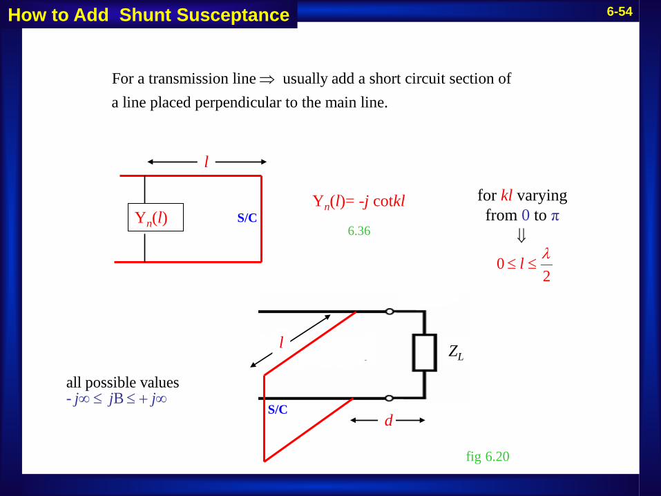
6-54How to Add Shunt Susceptance
For a transmission line usually add a short circuit section of a line placed perpendicular to the main line.
⇒
Yn(l)
l
Yn(l)= -j cotkl
ZLl
d
for kl varyingfrom 0 to π
fig 6.20
6.36
0
2
l λ
≤ ≤
⇓
all possible values- Bj j j∞ ≤ ≤ + ∞
S/C
S/C
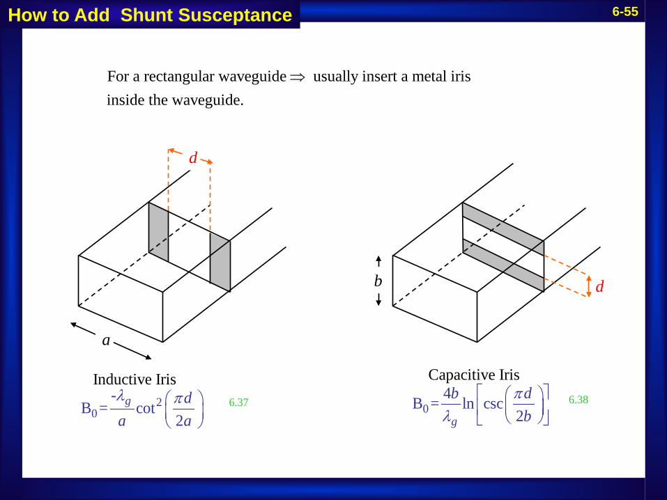
6-55How to Add Shunt Susceptance
For a rectangular waveguide usually insert a metal iris inside the waveguide.
⇒
6.3720
-B =
Inductive
cot2
Irisg d
a aλ π
a
d
d
b
6.380
Capacitive I4B = ln csc
s
2
ri
g
b db
πλ
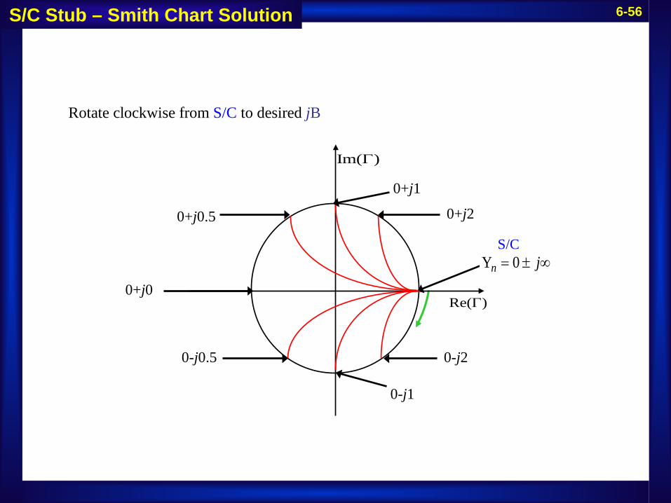
6-56S/C Stub – Smith Chart Solution
Rotate clockwise from to desirS/C ed Bj
S/C
0-j0.5
0-j1
0+j0.5
0+j1
0+j0
Y 0n j= ± ∞
Im( )Γ
Re( )Γ
0+j2
0-j2

6-57S/C Stub – Smith Chart Solution
Example: To add
B - 5 7 1.j j=
S/C
0 1.57j−
0.09λ
O/C Y cot
1.57 cot1cot 1.57 tan
1.57
2
analytically
;
[0.567
r
0.090
adian ]
3
s
n j klj j kl
kl kl
kl l
l
πλ
λ
= −− = −
= =
= =
=
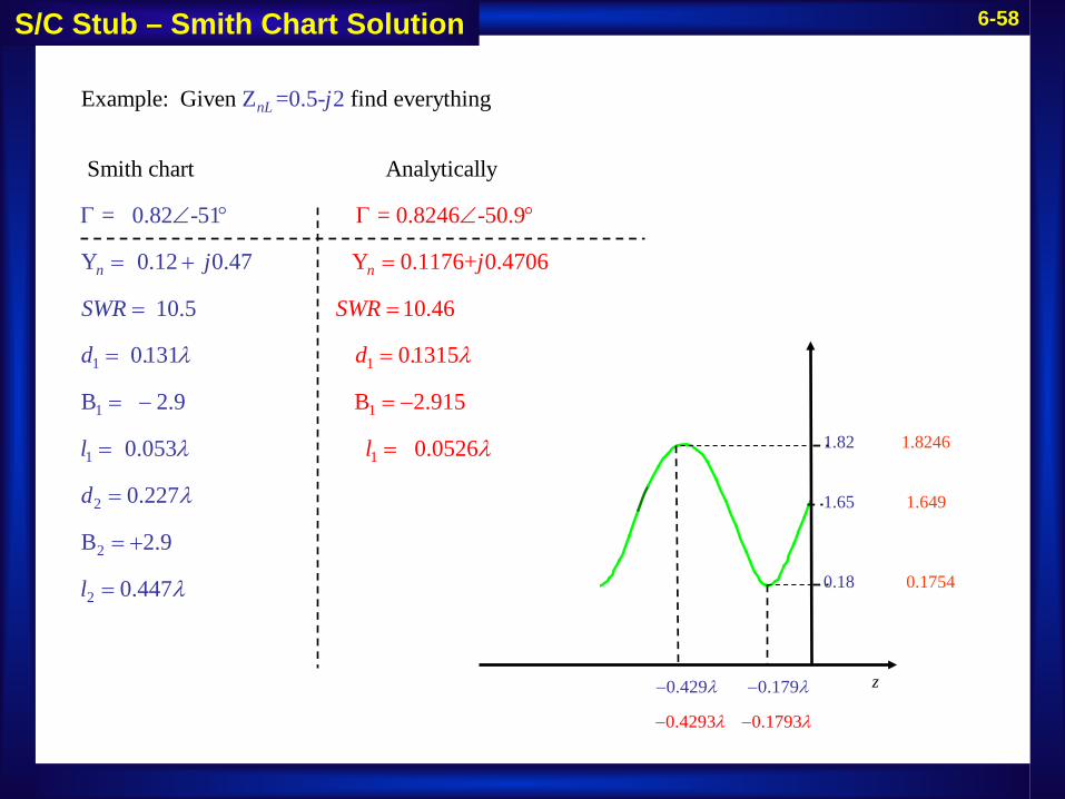
6-58S/C Stub – Smith Chart Solution
Example: Given find everything
Smith chart Analytica
=
Z =0.5- 2
0.8246 -50.9
Y 0.11
= 0.82 -51
Y 0.12 0.47
l
76+ 0.47
ly
nL
n n
j
j j
Γ
== +
Γ ∠ °∠ °
1
1
11
1
2
1
10.5
0.131
B 2.9
06
10.46
0.1315
B 2.915
0.053 0.05
0.2
26
27
B
SWR
d
l
SWR
d
l
d
λ
λ
λ
λ
λ
=
=
= −
=
=
=
=
= −
=
2
2
2.9
0.447l λ
= +
=
1+ LΓ
1- LΓ
z
ΓL
1.82
1.65
0.18
0.179λ−0.429λ−
0.4293λ−
1.8246
1.649
0.1754
0.1793λ−

6-59Smith Chart
fig 6.18
Y 0.12 0. 7 4nL j= +1 2.9j+
Z 0.5 2nL j= −
0.071λ
0.202λ
0.298λ
1 2.9j−
1 0.131d λ=2 0.227d λ=
0.82 51Γ = ∠− °

6-60Smith Chart
2.9j
0.197λ
0.303λ
2.9j− 1l
S/C
2l
1
1
(0.303 0.25)0.053
ll
λλ
= −=
2
2
(0.197 0.25)0.447
ll
λλ
= +=
1 2
N0
:.5
otell λ+ =


![Lambda Calculus - SJTUyuxi/teaching/lectures/Lambda Calculus.pdf · Lambda Calculus Alonzo Church [14Jun.1903-11Aug.1995] invented the -Calculus with a foundational motivation [1932].](https://static.fdocument.org/doc/165x107/5fb2b5193e095c5efe6ac4f7/lambda-calculus-sjtu-yuxiteachinglectureslambda-calculuspdf-lambda-calculus.jpg)