Chapter 6.

Laser: Theory and Applications

Reading: Sigman, Chapter 6, 7, and 26Bransden & Joachain, Chapter 15

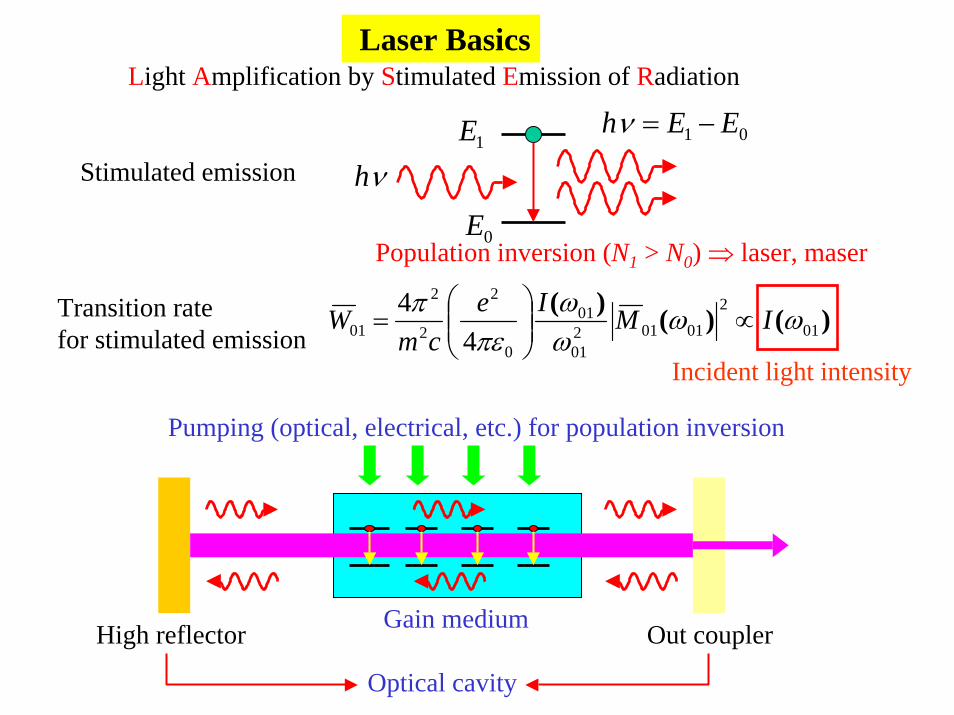
Laser Basics

Stimulated emission01 EEh −=ν

1E

0Eνh

Population inversion (N1 > N0) ⇒ laser, maser

Light Amplification by Stimulated Emission of Radiation

Transition rate for stimulated emission

)()()(01

201012

01

01

0

2

2

2

01 44 ωω

ωω

πεπ IMIe

cmW ∝⎟⎟

⎠

⎞⎜⎜⎝

⎛=

Incident light intensity

Gain mediumHigh reflector Out coupler

Optical cavity

Pumping (optical, electrical, etc.) for population inversion

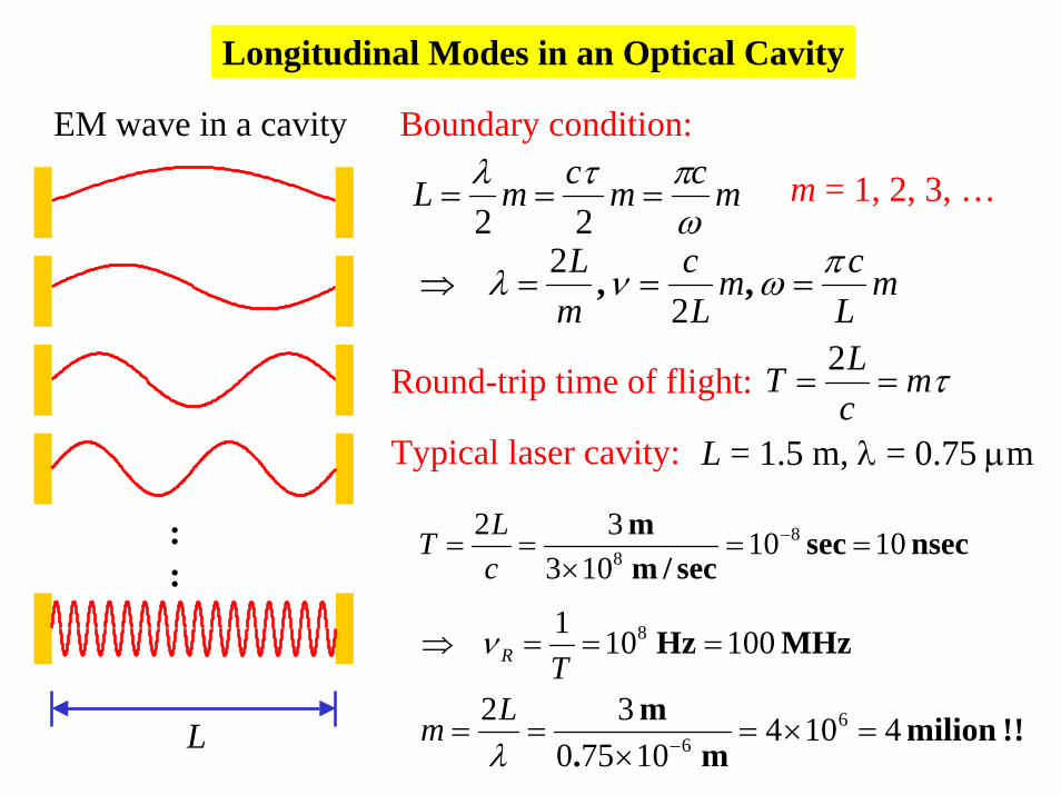
Longitudinal Modes in an Optical Cavity

Boundary condition:

::

L

EM wave in a cavity

mcmcmLωπτλ

===22

mLcm

Lc

mL πωνλ ===⇒ ,,

22

m = 1, 2, 3, …

Round-trip time of flight: τmcLT ==

2

Typical laser cavity: L = 1.5 m, λ = 0.75 µm

nsec secsec/m

m 1010103

32 88 ==

×== −

cLT

!! milion m.

m 410410750

32 66 =×=

×== −λ

Lm

MHz Hz 100101 8 ===⇒TRν

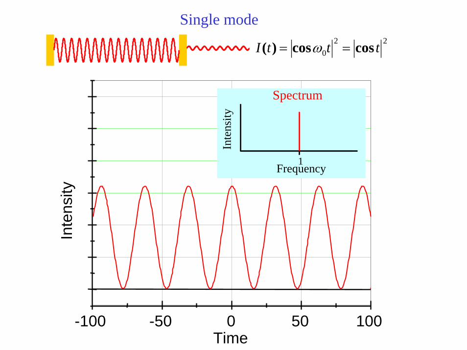
Single mode22

0 tttI coscos)( == ω

-100 -50 0 50 100Time

Inte

nsity

Frequency1

Inte

nsity

Spectrum

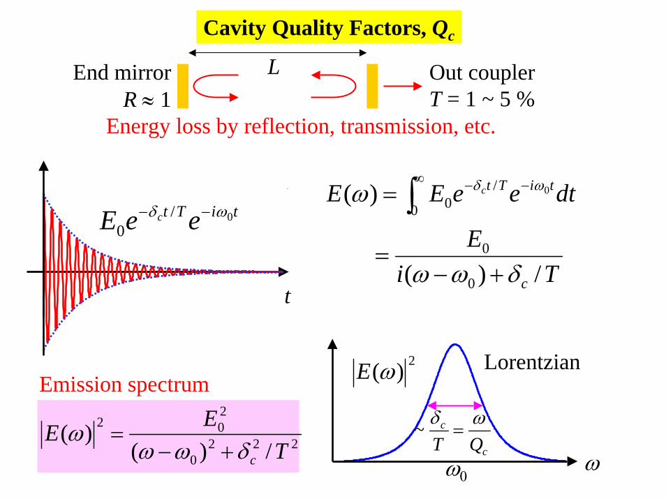
Cavity Quality Factors, Qc

End mirrorR ≈ 1

Out couplerT = 1 ~ 5 %

L

Energy loss by reflection, transmission, etc.

t

tiTt eeE c 0/0

ωδ −−

TiE

dteeEE

c

tiTtc

/)(

)(

0

0

0

/0

0

δωω

ω ωδ

+−=

= ∫∞ −−

2220

202

/)()(

TEE

cδωωω

+−=

Emission spectrum

ωω0

c

c

QTωδ

=~

2)(ωE Lorentzian

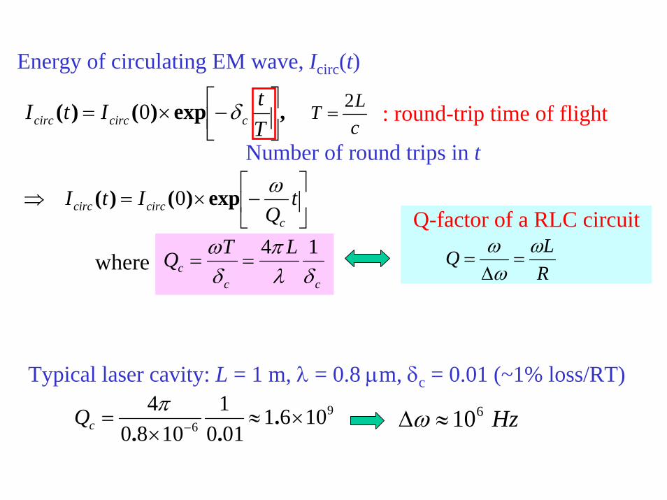
Energy of circulating EM wave, Icirc(t)

,exp)()( ⎥⎦⎤

⎢⎣⎡−×=

TtItI ccirccirc δ0

Number of round trips in t

: round-trip time of flightcLT 2

=

⎥⎦

⎤⎢⎣

⎡−×=⇒ t

QItI

ccirccirc

ωexp)()( 0

wherecc

cLTQ

δλπ

δω 14

==

Q-factor of a RLC circuit

RLQ ω

ωω

=∆

=

Typical laser cavity: L = 1 m, λ = 0.8 µm, δc = 0.01 (~1% loss/RT)9

6 10610101

10804

×≈×

= − ...

πcQ Hz610≈∆ω

[ ] )()()()()()(

)()(

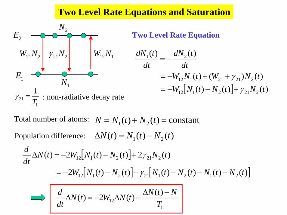
2212112

22121112

21

tNtNtNWtNWtNW

dttdN

dttdN

γγ+−−=

++−=

−=

Two Level Rate Equation

Two Level Rate Equations and Saturation

1E

2E

221NW 221Nγ

2N

1N

112NW

: non-radiative decay rate1

211T

=γ

Total number of atoms: constant)()( 21 =+= tNtNN

Population difference: )()()( 21 tNtNtN −=∆

[ ][ ] [ ])()()()()()(2

)(2)()(2)(

2121212112

2212112

tNtNtNtNtNtNW

tNtNtNWtNdtd

−−−−−−=

+−−=∆

γ

γ

112

)()(2)(T

NtNtNWtNdtd −∆

−∆−=∆

Steady-State Atomic Response: Saturation

112

)()(20)(T

NtNtNWtNdtd −∆

−∆−==∆

TWNNN ss

1221+=∆=∆

112 21,

/11

TW

WWNN

satsat

ss ≡+

=∆

0.01 0.1 1 100.0

0.2

0.4

0.6

0.8

1.0

1.2

NNss∆

TW122Signal strength,

SaturationIntensity, I=Isat

Gain coefficientin laser materials

Nm ∆∝α

sat

mm II

I/1

)( 0

+=

αα

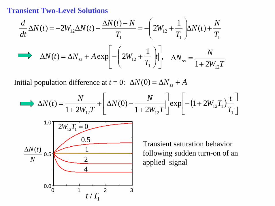
Transient Two-Level Solutions

1112

112 )(12)()(2)(

TNtN

TW

TNtNtNWtN

dtd

+∆⎟⎟⎠

⎞⎜⎜⎝

⎛+−=

−∆−∆−=∆

,12exp)(1

12 ⎥⎦

⎤⎢⎣

⎡⎟⎟⎠

⎞⎜⎜⎝

⎛+−+∆=∆ t

TWANtN ss

TWNNss

1221+=∆

Initial population difference at t = 0: ANN ss +∆=∆ )0(

( ) ⎥⎦

⎤⎢⎣

⎡+−⎥

⎦

⎤⎢⎣

⎡+

−∆++

=∆1

1121212

21exp21

)0(21

)(TtTW

TWNN

TWNtN

0 1 2 30.0

0.5

1.0

NtN )(∆

1/Tt

Transient saturation behavior following sudden turn-on of an applied signal

02 112 =TW

5.0124

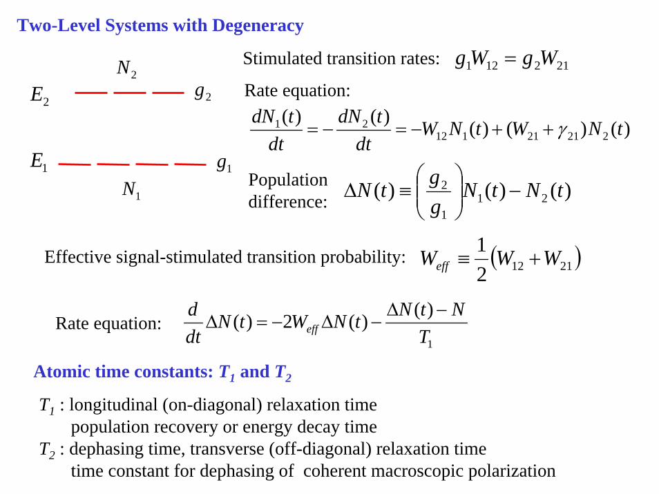
Two-Level Systems with Degeneracy

1E

2E 2g

1N1g

2N

)()()( 211

2 tNtNggtN −⎟⎟

⎠

⎞⎜⎜⎝

⎛≡∆Population

difference:

Stimulated transition rates: 212121 WgWg =

)()()()()(22121112

21 tNWtNWdt

tdNdt

tdN γ++−=−=

Rate equation:

Effective signal-stimulated transition probability: ( )211221 WWWeff +≡

1

)()(2)(T

NtNtNWtNdtd

eff−∆

−∆−=∆Rate equation:

Atomic time constants: T1 and T2

T1 : longitudinal (on-diagonal) relaxation timepopulation recovery or energy decay time

T2 : dephasing time, transverse (off-diagonal) relaxation timetime constant for dephasing of coherent macroscopic polarization

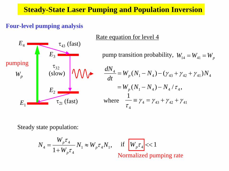
Rate equation for level 4

pWWW == 4114

,/)(

)()(

4441

4414243414

τ

γγγ

NNNW

NNNWdt

dN

p

p

−−=

++−−=

41424344

1 γγγγτ

++=≡where

pump transition probability,

Steady-State Laser Pumping and Population Inversion

Four-level pumping analysis

E1

E2

E3

E4 τ43 (fast)

τ32(slow)

τ21 (fast)

Wp

pumping

Steady state population:

,1 141

4

44 NWN

WW

N pp

p ττ

τ≈

+= if 14 <<τpW

Normalized pumping rate

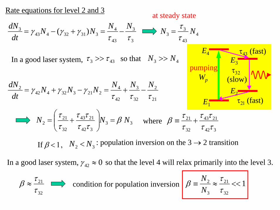
21

2

32

3

42

4221332442

2

τττγγγ NNNNNN

dtdN

−+=−+=

33342

2143

32

212 NNN β

ττττ

ττ

=⎟⎟⎠

⎞⎜⎜⎝

⎛+=

342

2143

32

21

ττττ

ττβ +≡where

If β < 1, 32 NN < : population inversion on the 3 → 2 transition

In a good laser system, 43 NN >>433 ττ >> so that

Rate equations for level 2 and 3

3

3

43

433132443

3 )(ττ

γγγ NNNNdt

dN−=+−=

at steady state

443

33 NN

ττ

=

E1

E2

E3

E4 τ43 (fast)

τ32(slow)

τ21 (fast)

Wp

pumping

In a good laser system, 042 ≈γ so that the level 4 will relax primarily into the level 3.

32

21

ττβ ≈ condition for population inversion 1

32

21

3

2 <<≈≡ττβ

NN

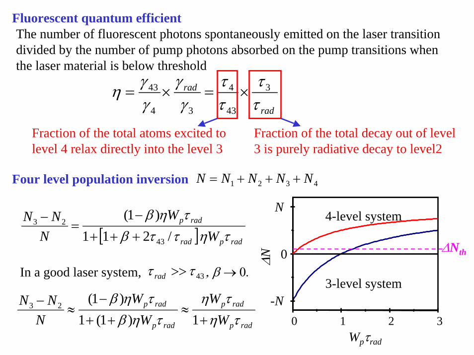
Fluorescent quantum efficient

rad

rad

ττ

ττ

γγ

γγη 3

43

4

34

43 ×=×=

The number of fluorescent photons spontaneously emitted on the laser transition divided by the number of pump photons absorbed on the pump transitions when the laser material is below threshold

Fraction of the total atoms excited to level 4 relax directly into the level 3

Fraction of the total decay out of level 3 is purely radiative decay to level2

Four level population inversion

[ ] radprad

radp

WW

NNN

τηττβτηβ

/211)1(

43

23

+++

−=

−

4321 NNNNN +++=

In a good laser system, 43ττ >>rad

radp

radp

radp

radp

WW

WW

NNN

τητη

τηβτηβ

+≈

++

−≈

−1)1(1

)1(23

, β → 0.3-level system

0 1 2 3

-N

0

N

∆N

Wpτrad

4-level system

∆Nth

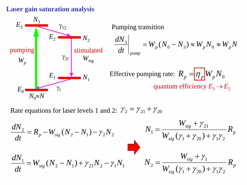
Laser gain saturation analysis

E0

E1

E2

E3 γ32

γ21

γ1

Wp

pumping

N0≈N

N1

N2

N3

Wsig

stimulated

Pumping transition

NWNWNNWdt

dNppp

pump

≈≈−= 0303 )(

0NWR ppp η=Effective pumping rate:

quantum efficiency E3 → E2

22122 )( NNNWR

dtdN

sigp γ−−−=

Rate equations for laser levels 1 and 2:

11221121 )( NNNNW

dtdN

sig γγ −+−=

20212 γγγ +=

psig

sig RW

WN

21201

211 )( γγγγ

γ++

+=

psig

sig RW

WN

21201

12 )( γγγγ

γ++

+=

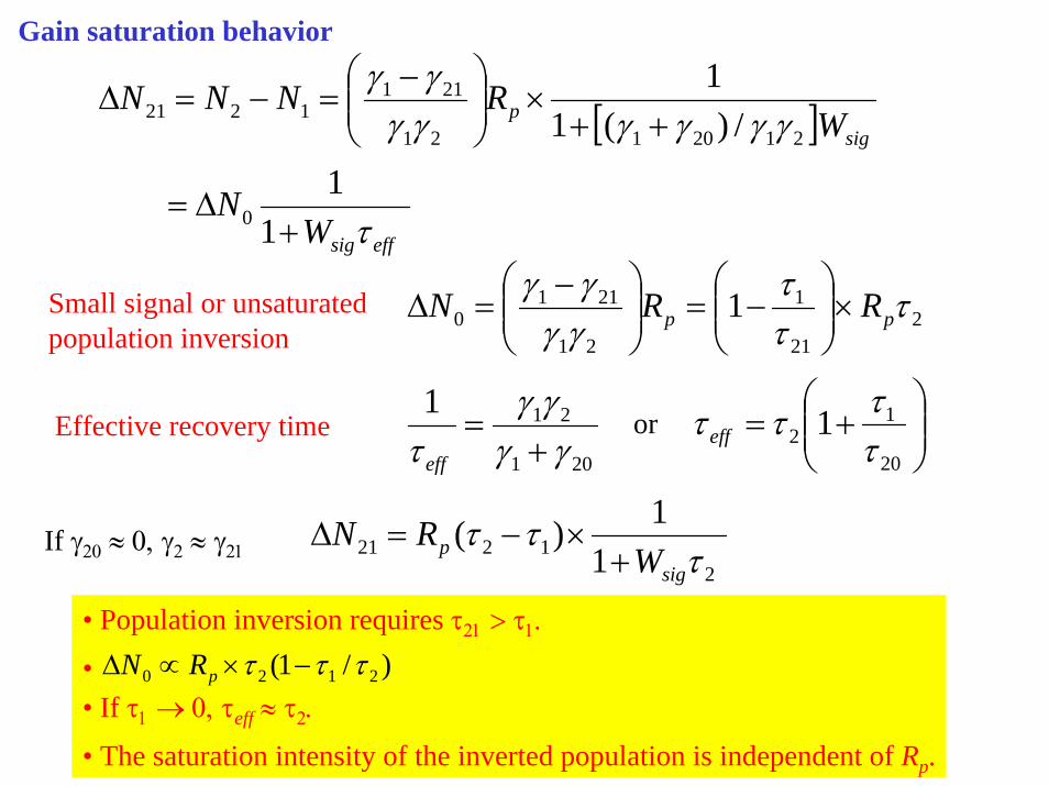
Gain saturation behavior

[ ]

effsig

sigp

WN

WRNNN

τ

γγγγγγγγ

+∆=

++×⎟⎟

⎠

⎞⎜⎜⎝

⎛ −=−=∆

11

/)(11

0

2120121

2111221

Small signal or unsaturated population inversion

221

1

21

2110 1 τ

ττ

γγγγ

pp RRN ×⎟⎟⎠

⎞⎜⎜⎝

⎛−=⎟⎟

⎠

⎞⎜⎜⎝

⎛ −=∆

Effective recovery time201

211γγ

γγτ +

=eff

⎟⎟⎠

⎞⎜⎜⎝

⎛+=

20

12 1

ττττ effor

If γ20 ≈ 0, γ2 ≈ γ212

1221 11)(

τττ

sigp W

RN+

×−=∆

• Population inversion requires τ21 > τ1.

•• If τ1 → 0, τeff ≈ τ2.

• The saturation intensity of the inverted population is independent of Rp.

)/1( 2120 τττ −×∝∆ pRN

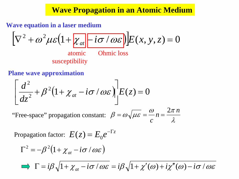
Wave Propagation in an Atomic Medium

Wave equation in a laser medium

( )[ ] 0),,(/122 =−++∇ zyxEiat ωεσχµεωOhmic lossatomic

susceptibility

( ) 0)(/122

2

=⎥⎦

⎤⎢⎣

⎡−++ zEi

dzd

at ωεσχβ

Plane wave approximation

“Free-space” propagation constant:λπωµεωβ nn

c2

===

Propagation factor:

( )ωεσχβ /122 iat −+−=Γ

zeEzE Γ−= 0)(

ωεσωχωχβωεσχβ /)()(1/1 iiiii at −′′+′+=−+=Γ

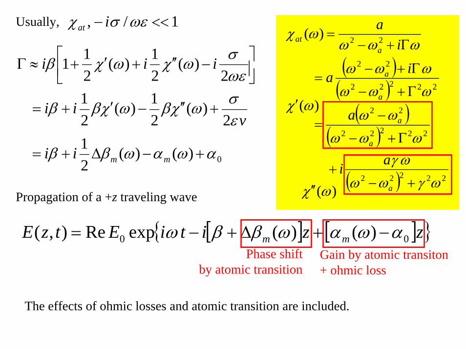
1/, <<− ωεσχ iatUsually,

0)()(21

2)(

21)(

21

2)(

21)(

211

αωαωββ

εσωχβωχββ

ωεσωχωχβ

+−∆+=

+′′−′+=

⎥⎦⎤

⎢⎣⎡ −′′+′+≈Γ

mmii

vii

iii

Propagation of a +z traveling wave

[ ] [ ]{ }zzitiEtzE mm 00 )()(expRe),( αωαωββω −+∆+−=

The effects of ohmic losses and atomic transition are included.

Phase shiftby atomic transition

Gain by atomic transiton+ ohmic loss

( )( )

( )( )

( ) 22222

22222

22

22222

22

22)(

ωγωωωγ

ωωωωω

ωωωωωω

ωωωωχ

+−+

Γ+−

−=

Γ+−

Γ+−=

Γ+−=

a

a

a

a

a

aat

ai

a

ia

ia

)(ωχ′

)(ωχ ′′

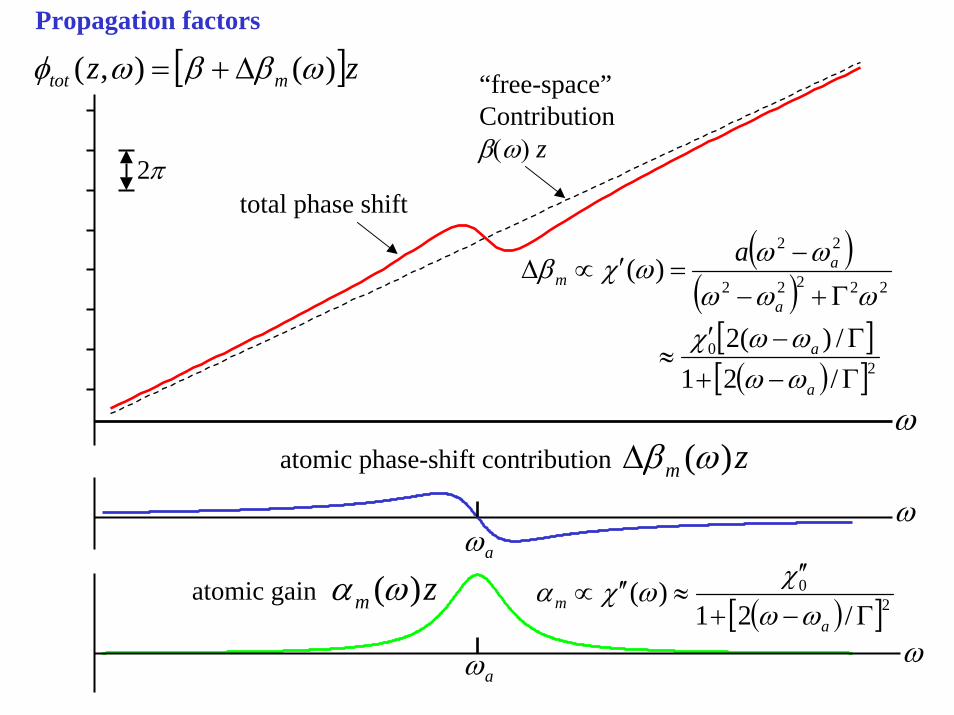
atomic phase-shift contribution zm )(ωβ∆

aωω

Propagation factors

[ ]zz mtot )(),( ωββωφ ∆+=

π2total phase shift

“free-space”Contributionβ(ω) z

ω

( )( )

[ ]( )[ ]2

0

22222

22

/21/)(2

)(

Γ−+Γ−′

≈

Γ+−

−=′∝∆

a

a

a

am

a

ωωωωχ

ωωωωωωχβ

aω

atomic gain zm )(ωα

ω( )[ ]2

0

/21)(

Γ−+

′′≈′′∝

am ωω

χωχα

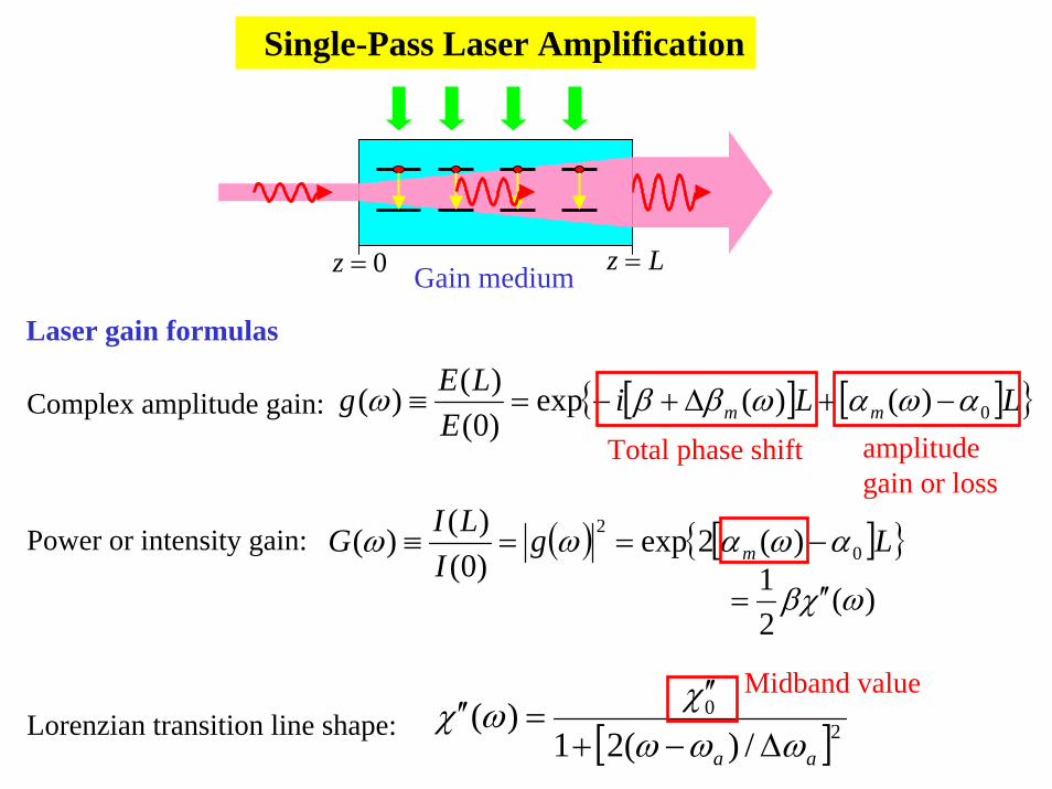
Single-Pass Laser Amplification

Gain medium0=z Lz =

Laser gain formulas

Complex amplitude gain: [ ] [ ]{ }LLiE

LEg mm 0)()(exp)0()()( αωαωββω −+∆+−=≡

Total phase shift amplitude gain or loss

Power or intensity gain: ( ) [ ]{ }LgI

LIG m 02 )(2exp

)0()()( αωαωω −==≡

)(21 ωχβ ′′=

Lorenzian transition line shape: [ ]20

/)(21)(

aa ωωωχωχ

∆−+

′′=′′

Midband value

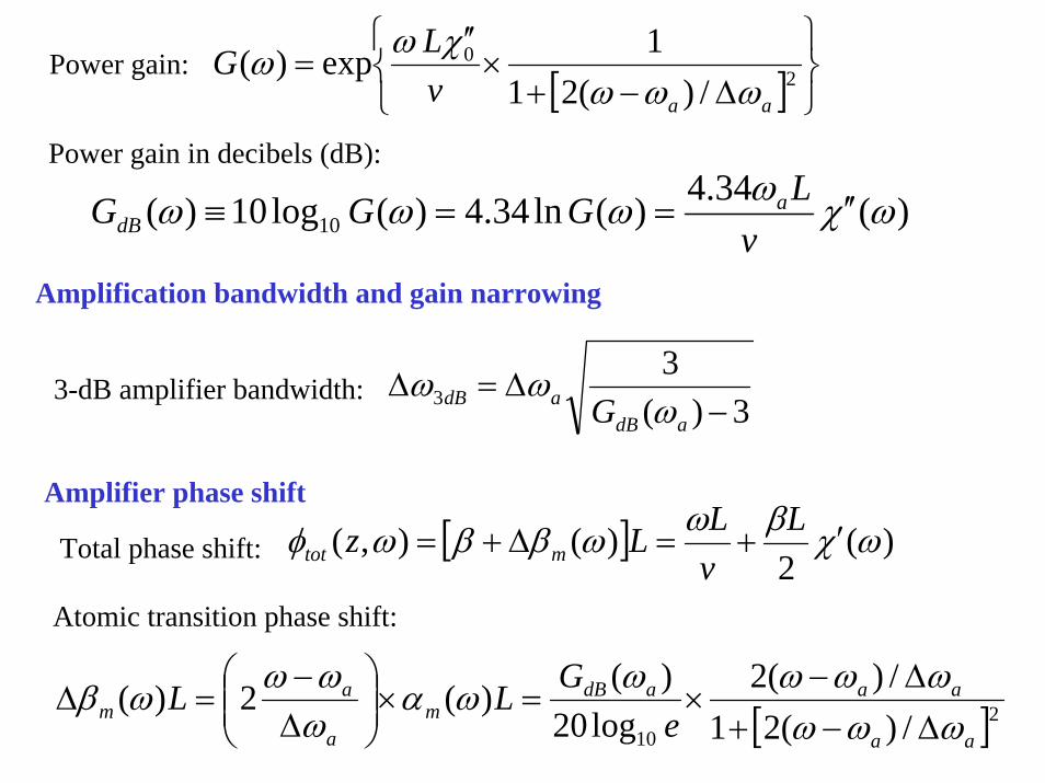
Power gain:[ ] ⎭

⎬⎫

⎩⎨⎧

∆−+×

′′= 2

0

/)(211exp)(

aavLG

ωωωχωω

Power gain in decibels (dB):

)(34.4)(ln34.4)(log10)( 10 ωχωωωω ′′==≡v

LGGG adB

Amplification bandwidth and gain narrowing

3-dB amplifier bandwidth:3)(

33 −

∆=∆adB

adB G ωωω

Amplifier phase shift

[ ] )(2

)(),( ωχβωωββωφ ′+=∆+=L

vLLz mtotTotal phase shift:

[ ]210 /)(21

/)(2log20

)()(2)(aa

aaadBm

a

am e

GLLωωω

ωωωωωαωωωωβ

∆−+∆−

×=×⎟⎟⎠

⎞⎜⎜⎝

⎛∆−

=∆

Atomic transition phase shift:

Saturation Intensities in Laser Materials

Saturation of the population difference

sateff IIN

WNN

/11

11

00 +×∆=

+×∆=∆

τ

INIdzdI

m σα ∆== 2Traveling wave:Stimulated transition cross-section

Population difference:

sat

mm IzI

zdz

zdIzI /)(1

2)(2)()(

1 0

+==

αα σα 002 Nm ∆≡where

∫∫ =⎥⎦

⎤⎢⎣

⎡+

=

=

L

m

II

IIsat

dzdIII

out

in 00211 α

00 ln2ln GLI

IIII

msat

inout

in

out ==−

+⎟⎟⎠

⎞⎜⎜⎝

⎛α where )2exp( 00 LG mα≡

unsaturatedpower gain

⎥⎦

⎤⎢⎣

⎡ −−×=⎥

⎦

⎤⎢⎣

⎡ −−×=

⎥⎦

⎤⎢⎣

⎡ −−×=≡

sat

out

sat

in

sat

inout

in

out

GIIGG

IIGG

IIIG

IIG

)1(exp)1(exp

exp

00

0

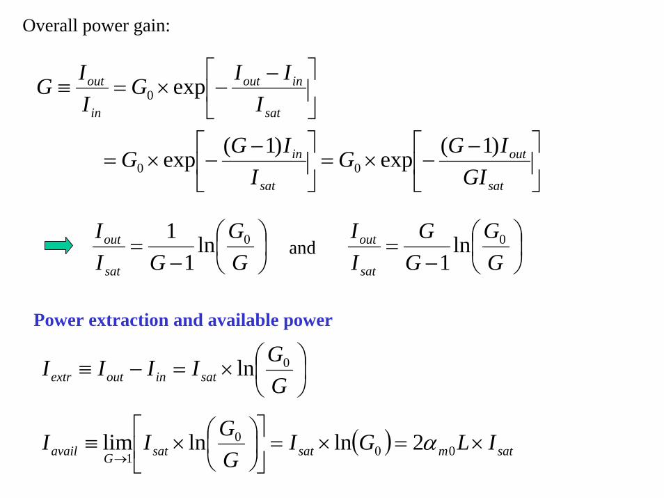
Overall power gain:

⎟⎠⎞

⎜⎝⎛

−=

GG

GII

sat

out 0ln1

1⎟⎠⎞

⎜⎝⎛

−=

GG

GG

II

sat

out 0ln1

and

Power extraction and available power

⎟⎠⎞

⎜⎝⎛×=−≡

GGIIII satinoutextr

0ln

( ) satmsatsatGavail ILGIGGII ×=×=⎥

⎦

⎤⎢⎣

⎡⎟⎠⎞

⎜⎝⎛×≡

→ 000

12lnlnlim α

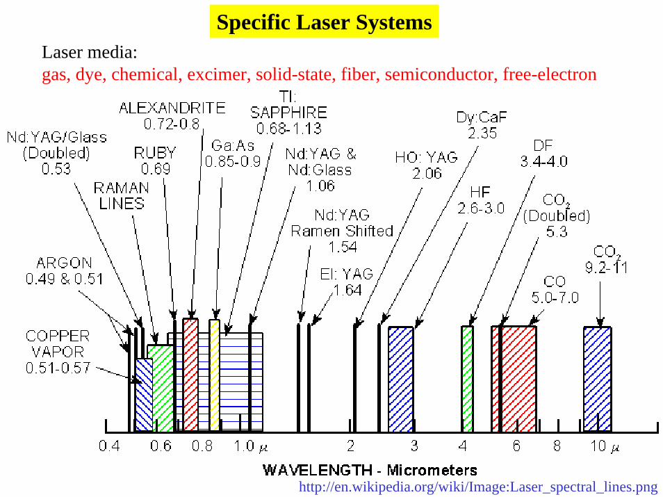
Specific Laser SystemsLaser media: gas, dye, chemical, excimer, solid-state, fiber, semiconductor, free-electron

http://en.wikipedia.org/wiki/Image:Laser_spectral_lines.png

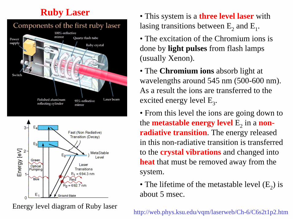
Ruby Laser

http://web.phys.ksu.edu/vqm/laserweb/Ch-6/C6s2t1p2.htmEnergy level diagram of Ruby laser

• This system is a three level laser with lasing transitions between E2 and E1. • The excitation of the Chromium ions is done by light pulses from flash lamps (usually Xenon). • The Chromium ions absorb light at wavelengths around 545 nm (500-600 nm). As a result the ions are transferred to the excited energy level E3. • From this level the ions are going down to the metastable energy level E2 in a non-radiative transition. The energy released in this non-radiative transition is transferred to the crystal vibrations and changed into heat that must be removed away from the system. • The lifetime of the metastable level (E2) is about 5 msec.

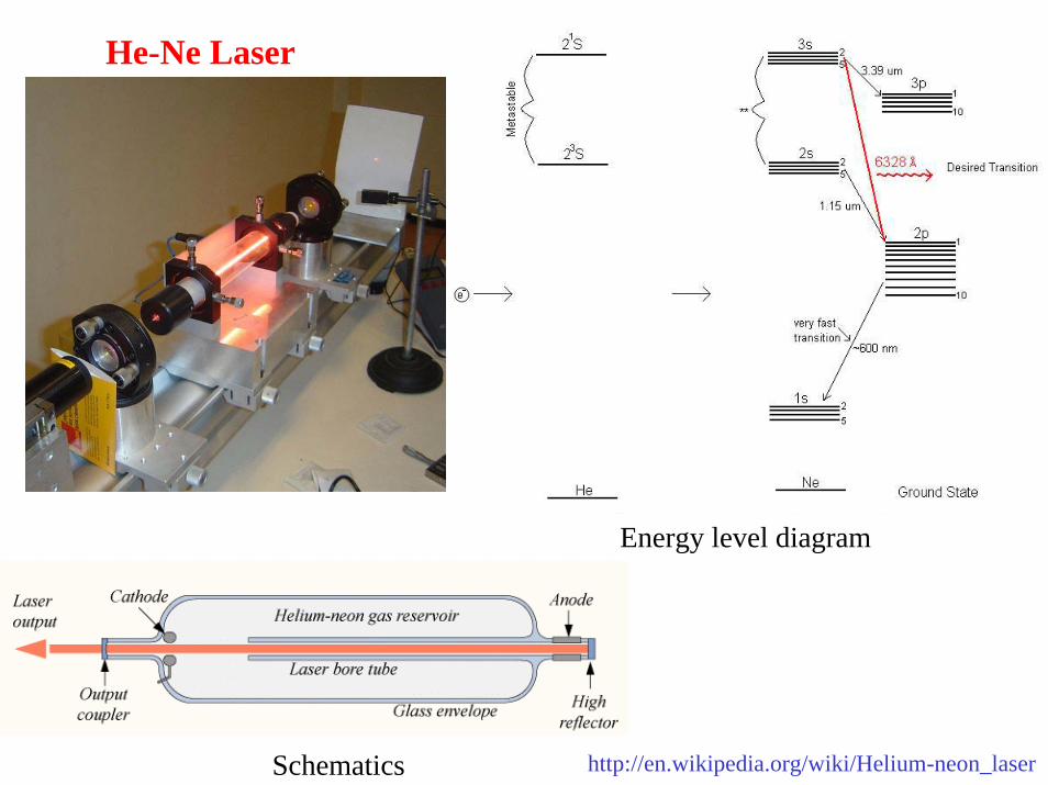
He-Ne Laser

Energy level diagram

Schematics http://en.wikipedia.org/wiki/Helium-neon_laser

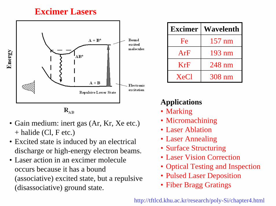
Excimer Lasers

Applications• Marking • Micromachining • Laser Ablation • Laser Annealing • Surface Structuring • Laser Vision Correction • Optical Testing and Inspection • Pulsed Laser Deposition • Fiber Bragg Gratings

• Gain medium: inert gas (Ar, Kr, Xe etc.) + halide (Cl, F etc.)

• Excited state is induced by an electrical discharge or high-energy electron beams.

• Laser action in an excimer molecule occurs because it has a bound (associative) excited state, but a repulsive (disassociative) ground state.

Excimer WavelenthFe 157 nm

ArF 193 nmKrF 248 nm

XeCl 308 nm

http://tftlcd.khu.ac.kr/research/poly-Si/chapter4.html

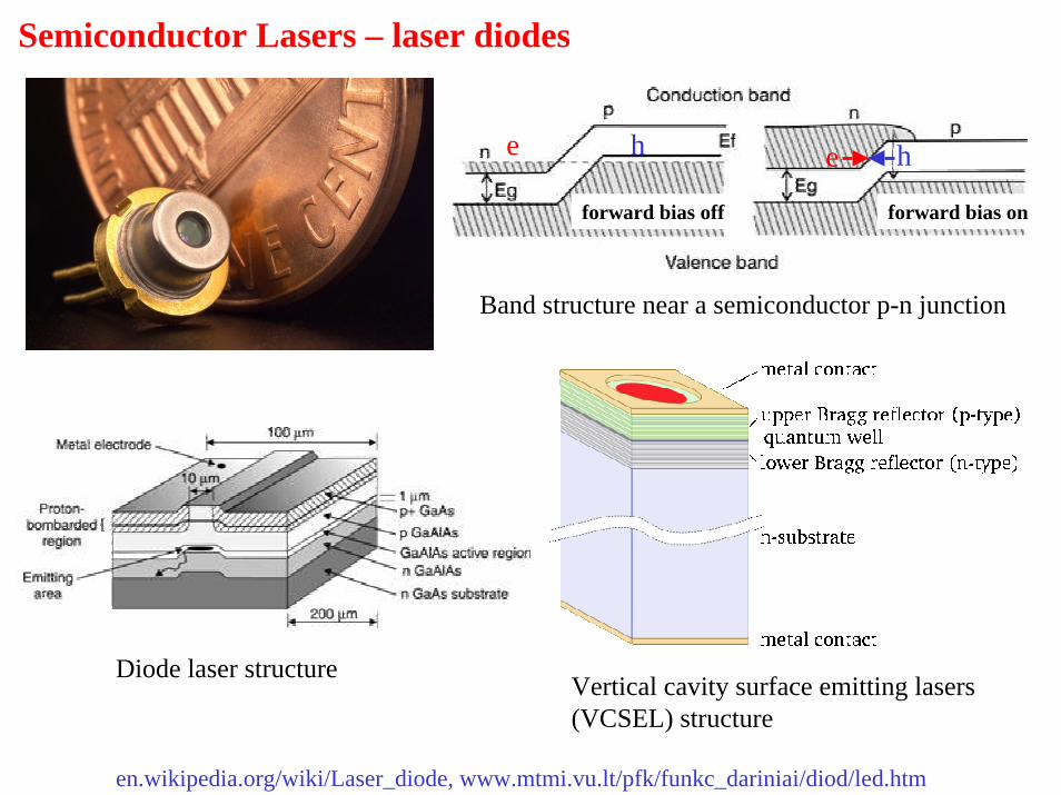
Semiconductor Lasers – laser diodes

Vertical cavity surface emitting lasers (VCSEL) structure

Band structure near a semiconductor p-n junction

e h e h

forward bias off forward bias on

Diode laser structure

en.wikipedia.org/wiki/Laser_diode, www.mtmi.vu.lt/pfk/funkc_dariniai/diod/led.htm

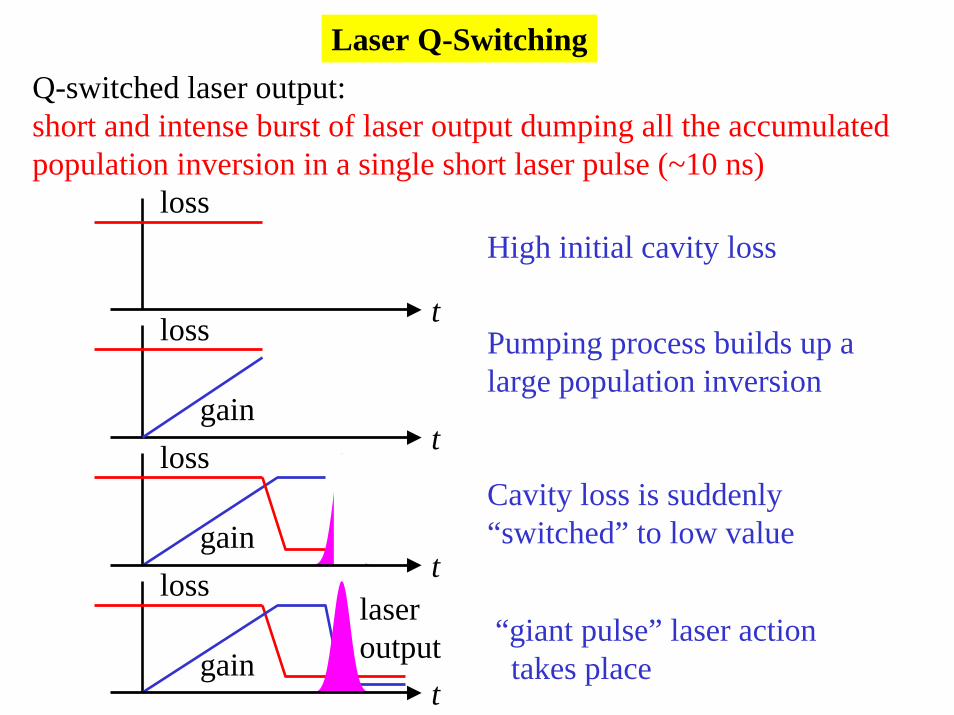
Laser Q-SwitchingQ-switched laser output: short and intense burst of laser output dumping all the accumulated population inversion in a single short laser pulse (~10 ns)

High initial cavity lossloss

gain

loss

loss

lossgain

gain

laseroutput

t

t

tPumping process builds up a large population inversion

t

Cavity loss is suddenly “switched” to low value

“giant pulse” laser action takes place

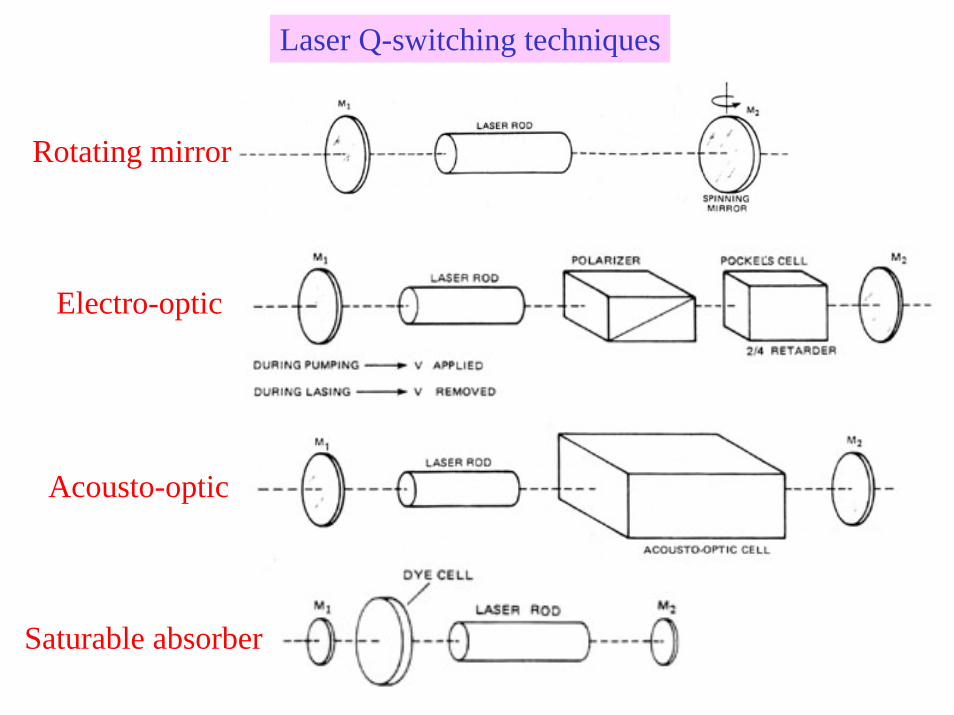
Laser Q-switching techniques

Rotating mirror

Electro-optic

Acousto-optic

Saturable absorber

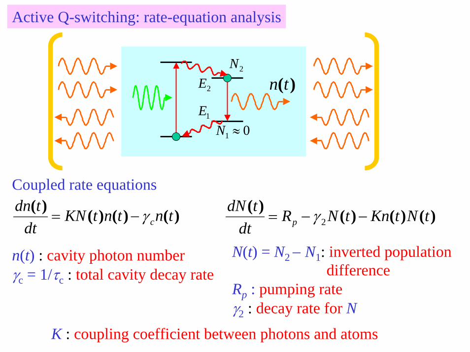
Active Q-switching: rate-equation analysis

2E

1E01 ≈N

2N)(tn

Coupled rate equations

)()()()( tNtKntNRdt

tdNp −−= 2γ)()()()( tntntKN

dttdn

cγ−=

N(t) = N2 − N1: inverted population difference

Rp : pumping rateγ2 : decay rate for N

n(t) : cavity photon numberγc = 1/τc : total cavity decay rate

K : coupling coefficient between photons and atoms

Pumping interval, and population build-up

gaint

lossPumping process builds up a large population inversion

n(t) = 0 and a pump pulse with constant intensity Rp is turned on at t = 0.

[ ])/exp()(/)()(222 1 τττ tRtNtNR

dttdN

pp −−=⇒−=

Pump Pulse Durationτ2 2τ2

2τpR

N(t)

Energy storage during the pumping interval for a fixed pumping rate

Typical solid state lasers: τ2 ≈ 200 µs

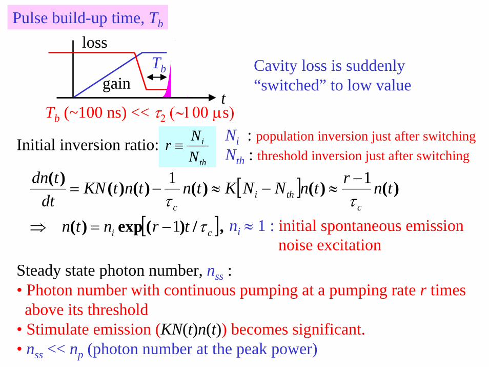
Pulse build-up time, Tb

Initial inversion ratio:th

i

NNr ≡

Ni : population inversion just after switchingNth : threshold inversion just after switching

[ ]

[ ],/)(exp)(

)()()()()()(

ci

cthi

c

trntn

tnrtnNNKtntntKNdt

tdn

τττ

1

11

−=⇒

−≈−≈−=

loss

gaint

Cavity loss is suddenly “switched” to low value

Tb

Tb (~100 ns) << τ2 (∼100 µs)

ni ≈ 1 : initial spontaneous emission noise excitation

Steady state photon number, nss : • Photon number with continuous pumping at a pumping rate r times above its threshold

• Stimulate emission (KN(t)n(t)) becomes significant.• nss << np (photon number at the peak power)

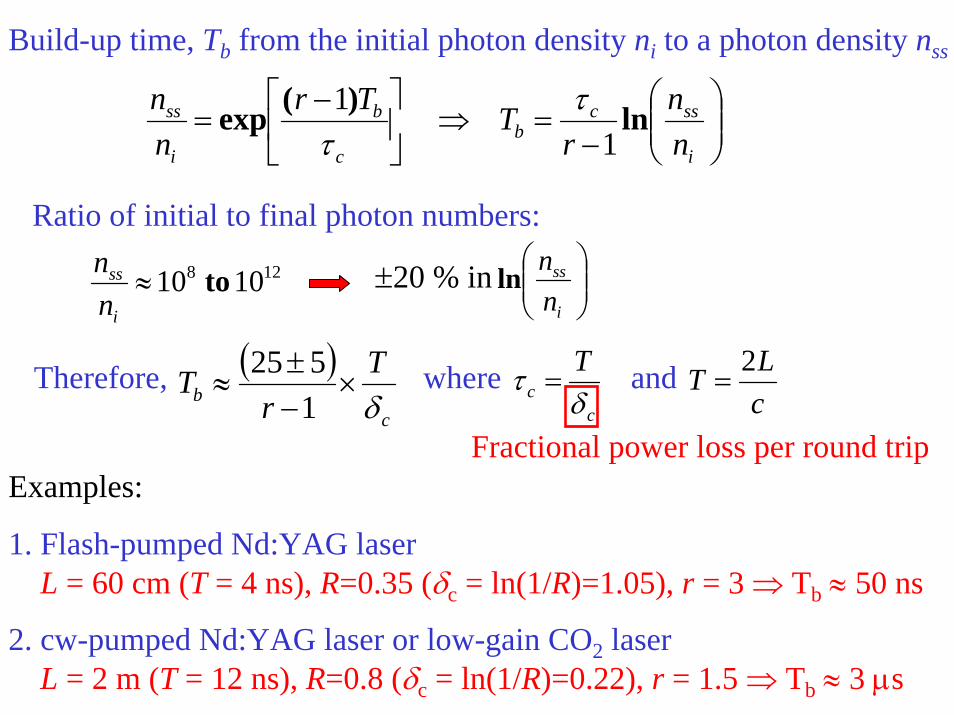
Build-up time, Tb from the initial photon density ni to a photon density nss

⎟⎟⎠

⎞⎜⎜⎝

⎛−

=⇒⎥⎦

⎤⎢⎣

⎡ −=

i

sscb

c

b

i

ss

nn

rTTr

nn ln)(exp

11 τ

τ

Ratio of initial to final photon numbers:128 1010 to≈

i

ss

nn ±20 % in ⎟⎟

⎠

⎞⎜⎜⎝

⎛

i

ss

nnln

( )c

bT

rT

δ×

−±

≈1525

cc

Tδ

τ =wherecLT 2

=

Fractional power loss per round trip

Therefore, and

Examples:

1. Flash-pumped Nd:YAG laserL = 60 cm (T = 4 ns), R=0.35 (δc = ln(1/R)=1.05), r = 3 ⇒ Tb ≈ 50 ns

2. cw-pumped Nd:YAG laser or low-gain CO2 laserL = 2 m (T = 12 ns), R=0.8 (δc = ln(1/R)=0.22), r = 1.5 ⇒ Tb ≈ 3 µs

Pulse output interval

[ ] )()()()()()( tnNtNKtntntKNdt

tdnthc −=−= γ

loss

gainlaseroutput

t )()()()()()( tNtKntNtKntNRdt

tdNp −≈−−= 2γ

at the switching time t = tiInitial conditions: thi rNNN == 1== innand

)(ln)()(

))(()(ln)()(

)()(

tNN

rNtNNtn

NtNN

tNNdNN

Ntn

dNN

NdnN

NNdNdn

iii

ii

th

tN

Nth

tN

Nthtn

nth

i

ii

−−≈⇒

−−=⎟⎠⎞

⎜⎝⎛ −≈⇒

⎟⎠⎞

⎜⎝⎛ −=⇒

−=

∫

∫∫

1

1

th

i

NNr =where

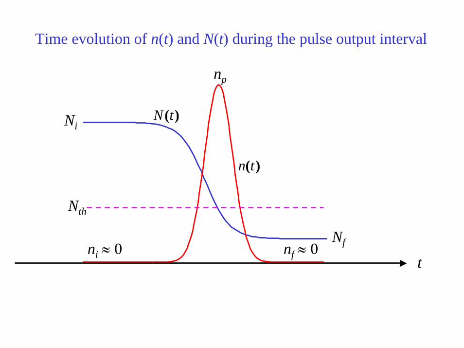
Time evolution of n(t) and N(t) during the pulse output interval

Ni

Nf

Nth

ni ≈ 0 nf ≈ 0

np

t

)(tN

)(tn

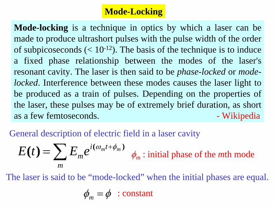
Mode-Locking

Mode-locking is a technique in optics by which a laser can be made to produce ultrashort pulses with the pulse width of the order of subpicoseconds (< 10-12). The basis of the technique is to induce a fixed phase relationship between the modes of the laser's resonant cavity. The laser is then said to be phase-locked or mode-locked. Interference between these modes causes the laser light to be produced as a train of pulses. Depending on the properties ofthe laser, these pulses may be of extremely brief duration, as short as a few femtoseconds. - Wikipedia

General description of electric field in a laser cavity

∑ +=m

tim

mmeEtE )()( φω

The laser is said to be “mode-locked” when the initial phases are equal.

φm : initial phase of the mth mode

φφ =m : constant

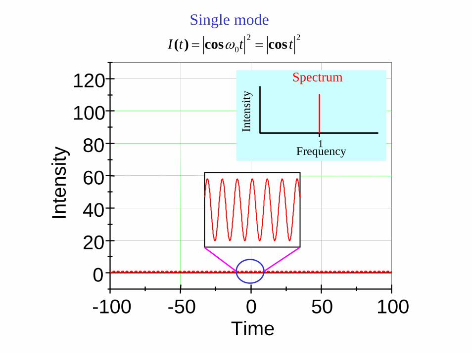
Single mode22

0 tttI coscos)( == ω

-100 -50 0 50 1000

20406080

100120

Time

Inte

nsity Frequency

1

Inte

nsity

Spectrum

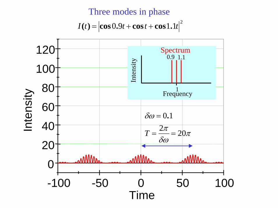
Three modes in phase21190 ttttI .coscos.cos)( ++=

-100 -50 0 50 1000

20406080

100120

Time

Inte

nsity Frequency

1

Inte

nsity

Spectrum0.9 1.1

πδω

πδω

20210

==

=

T

.

Eleven modes with random phases2

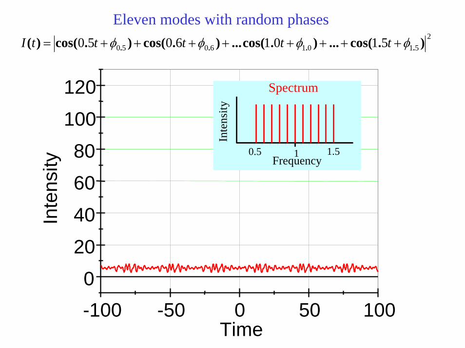
51016050 51016050 ).cos(...).cos(...).cos().cos()( .... φφφφ ++++++++= tttttI

-100 -50 0 50 1000

20406080

100120

Time

Inte

nsity Frequency

1

Inte

nsity

Spectrum

0.5 1.5

Eleven modes with the same phase, φ = 025141016050 ttttttI .cos.cos....cos....cos.cos)( ++++=

-100 -50 0 50 1000

20406080

100120

Time

Inte

nsity Frequency

1

Inte

nsity

Spectrum

0.5 1.5

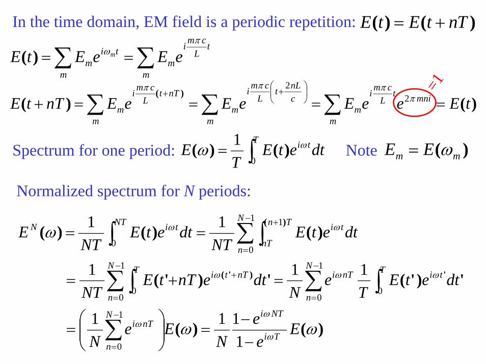
In the time domain, EM field is a periodic repetition: )()( TntEtE +=

∑∑ ==m

tL

cmi

mm

tim eEeEtE m

πω)(

)()()(

tEeeEeEeEnTtE mni

m

tL

cmi

mm m

cnLt

Lcmi

m

nTtL

cmi

m ====+ ∑∑ ∑⎟⎠⎞

⎜⎝⎛ ++ π

πππ2

2 =1

dtetET

ET ti∫=0

1 ωω )()( )( mm EE ω=Spectrum for one period: Note

Normalized spectrum for N periods:

)()(

')'(')'(

)()()(

')'(

)(

ωω

ω

ω

ωω

ωωω

ωω

Eee

NEe

N

dtetET

eN

dtenTtENT

dtetENT

dtetENT

E

Ti

NTiN

n

nTi

N

n

T tinTiN

n

T nTti

N

n

Tn

nT

tiNT tiN

−−

=⎟⎟⎠

⎞⎜⎜⎝

⎛=

=+=

==

∑

∑ ∫∑∫

∑∫∫

−

=

−

=

−

=

+

−

=

+

1111

111

11

1

0

1

00

1

00

1

0

1

0

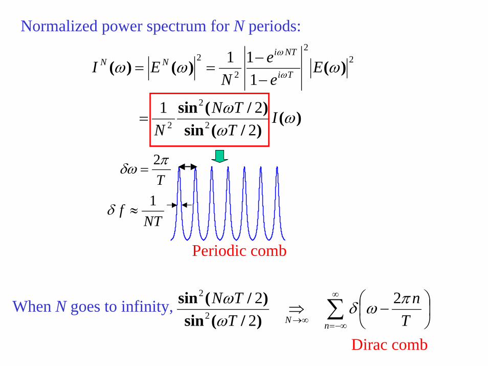
Normalized power spectrum for N periods:

)()/(sin)/(sin

)()()(

ωωω

ωωω ω

ω

ITTN

N

Eee

NEI Ti

NTiNN

221

111

2

2

2

22

2

2

=

−−

==

Periodic comb

Tπδω 2

=

NTf 1

≈δ

When N goes to infinity, ∑∞

−∞=∞→⎟⎠⎞

⎜⎝⎛ −⇒

nN Tn

TTN πωδ

ωω 2

22

2

2

)/(sin)/(sin

Dirac comb

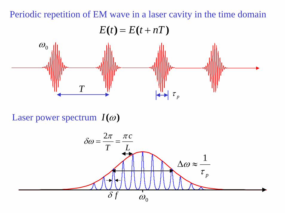
Periodic repetition of EM wave in a laser cavity in the time domain

)()( TntEtE +=

T

0ω

pτ

Laser power spectrum )(ωI

0ω

pτω 1

≈∆

Lc

Tππδω ==

2

fδ

-100 -50 0 50 100

Time

020406080

100120

Inte

nsity

020406080

100120

Inte

nsity

020406080

100120

Inte

nsity

020406080

100120

Inte

nsity

Frequency1

Inte

nsity

0.5 1.5

1

Inte

nsity

0.5 1.5

Inte

nsity

Inte

nsity

Spectrum

10.5 1.5

10.5 1.5

Eleven modesrandom phases

Eleven modessame phase

Singlemode

Threemodesin phase

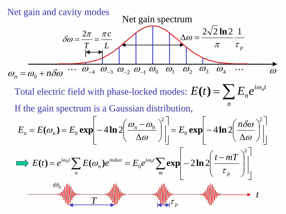
Net gain and cavity modes

Total electric field with phase-locked modes:

If the gain spectrum is a Gaussian distribution,

⎥⎥⎦

⎤

⎢⎢⎣

⎡⎟⎠⎞

⎜⎝⎛

∆−=

⎥⎥⎦

⎤

⎢⎢⎣

⎡⎟⎠⎞

⎜⎝⎛

∆−

−==2

0

20

0 2424ω

δωωωωω nEEEE n

nn lnexplnexp)(

∑∑ ⎥⎥

⎦

⎤

⎢⎢

⎣

⎡

⎟⎟⎠

⎞⎜⎜⎝

⎛ −−==

m p

ti

n

tinn

ti mTteEeEetE2

0 2200

τω ωδωω lnexp)()(

∑=n

tin

neEtE ω)(

0ω

pτπω 1222 ln

=∆Lc

Tππδω ==

2

ω1ω 3ω2ω 4ω1−ω2−ω4−ω 3−ω

Net gain spectrum

δωωω nn += 0……

T0ω

pτt

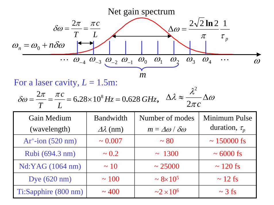
For a laser cavity, L = 1.5m:

pτπω 1222 ln

=∆Lc

Tππδω ==

2

ω

Net gain spectrum

δωωω nn += 0

……

m0ω 1ω 3ω2ω 4ω1−ω2−ω4−ω 3−ω

ωπλλ ∆≈∆

c2

2

Gain Medium(wavelength)

Bandwidth∆λ (nm)

Number of modesm = ∆ω / δω

Minimum Pulse duration, τp

Ar+-ion (520 nm) ~ 0.007 ~ 80 ~ 150000 fs

Rubi (694.3 nm) ~ 0.2 ~ 1300 ~ 6000 fs

Nd:YAG (1064 nm) ~ 10 ~ 25000 ~ 120 fs

Dye (620 nm) ~ 100 ~ 8×105 ~ 12 fs

Ti:Sapphire (800 nm) ~ 400 ~2 ×106 ~ 3 fs

,.. GHzHzLc

T6280102862 8 =×===

ππδω

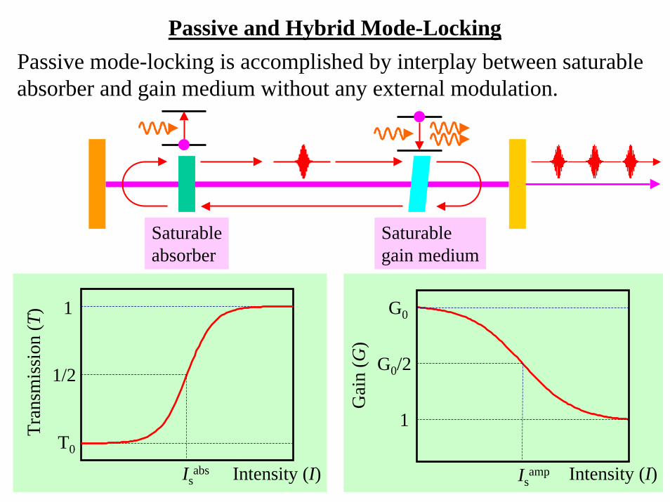
Passive and Hybrid Mode-LockingPassive mode-locking is accomplished by interplay between saturable absorber and gain medium without any external modulation.

Saturableabsorber

Saturablegain medium

T0

1

Intensity (I)Isabs

1/2

Tran

smis

sion

(T)

1

G0

Intensity (I)Isamp

G0/2G

ain

(G)

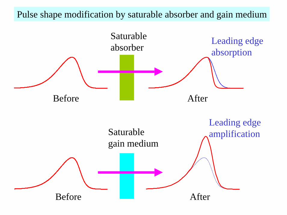
Pulse shape modification by saturable absorber and gain medium

Saturable absorber

Leading edgeabsorption

Before After

Leading edgeamplificationSaturable

gain medium

Before After

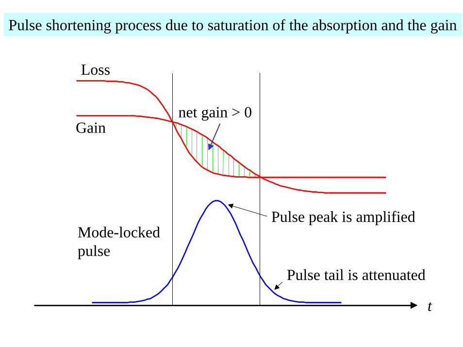
Pulse shortening process due to saturation of the absorption and the gain

Loss

Gainnet gain > 0

Pulse peak is amplified

Pulse tail is attenuated

Mode-lockedpulse

t

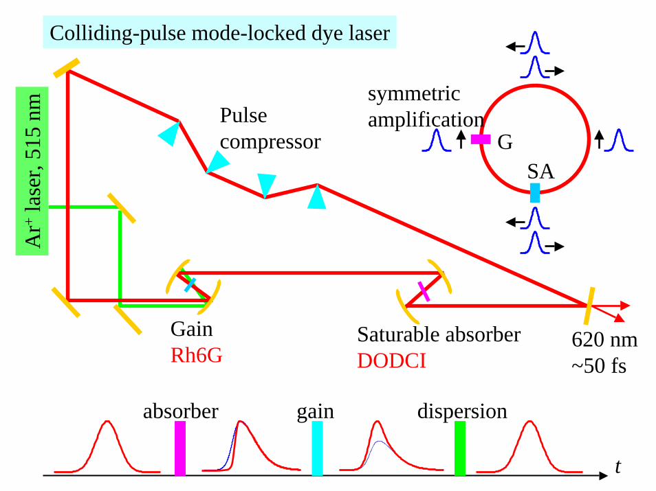
Colliding-pulse mode-locked dye laser

GSA

Ar+

lase

r, 51

5 nm Pulse

compressor

GainRh6G

Saturable absorberDODCI

620 nm~50 fs

symmetric amplification

absorber gain dispersion

t

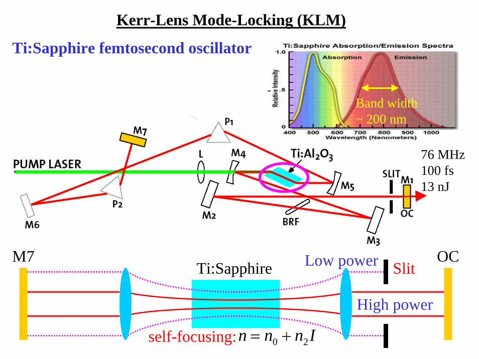
Kerr-Lens Mode-Locking (KLM)

Ti:Sapphire

High power

Low power

self-focusing:

SlitM7 OC

Ti:Sapphire femtosecond oscillator

76 MHz100 fs13 nJ

Band width~ 200 nm

Innn 20 +=

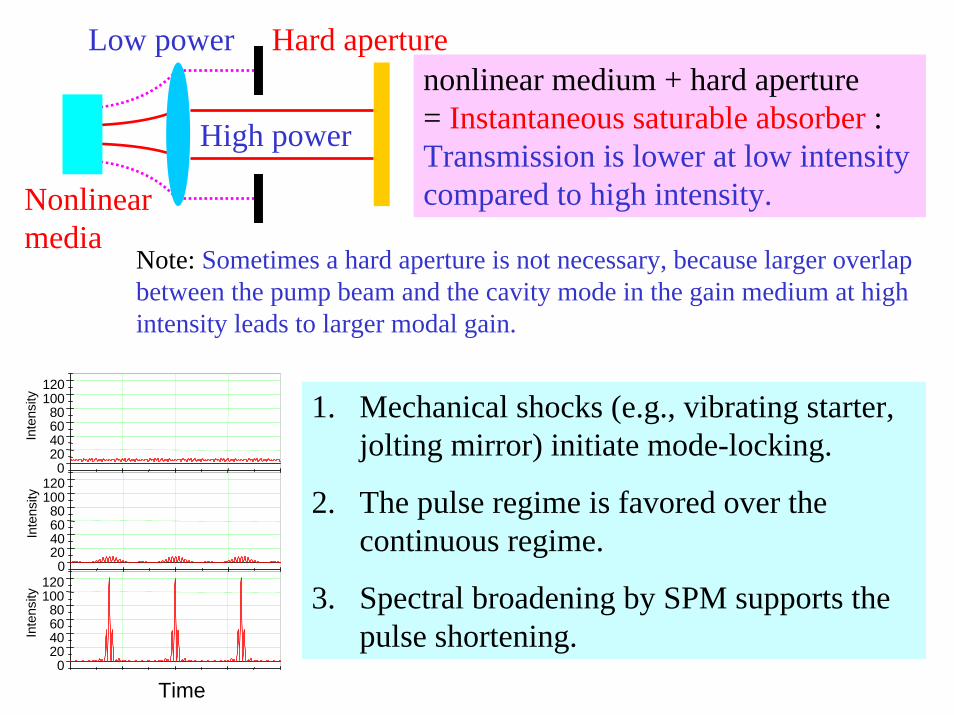
High power

Low power Hard aperturenonlinear medium + hard aperture= Instantaneous saturable absorber :Transmission is lower at low intensity compared to high intensity.Nonlinear

mediaNote: Sometimes a hard aperture is not necessary, because larger overlap between the pump beam and the cavity mode in the gain medium at high intensity leads to larger modal gain.

Time

020406080

100120

Inte

nsity

020406080

100120

Inte

nsity

020406080

100120

Inte

nsity 1. Mechanical shocks (e.g., vibrating starter,

jolting mirror) initiate mode-locking.

2. The pulse regime is favored over the continuous regime.

3. Spectral broadening by SPM supports the pulse shortening.