Chapter 5

Multifactor Pricing Models

5.1 Multifactor Pricing Models

Motivation: Empirical evidences show that the market β does not

completely explain the cross section risk; More factors are needed to

explain the cross-sectional risk.

Commonly-used factors:

— proxies of market portfolio;149

150

— Firm characteristics: “size e ect”, “PE e ect”, “book-marketff ffratios”:

*** size e ect: di erence of returns on a portfolio with small capi-ff fftalization and high capitalization;

*** PE e ect: di erence of returns on a portfolio with small PE andff ffhigh PE;

— Macroeconomic and market variables: “maturity premium”

(yield spread between long and short rates), expected inflation,

unexpected inflation, industrial production growth, “default pre-

mium” (yield spread between high and low grade bonds).

Notation:

151

— R = (R1, · · · , RN )T is a vector of returns of N traded assets.

— f is the measurements (returns) related to K common factors.

The Models: The cross-sectional risk is modelled as

R = a + Bf + ε,

E(ε) = 0, Var(ε) = Σ.

For example, the return of the ith portfolio is

Rit = ai + bi1f1t + · · · + biKfKt + εit, t = 1, · · · , T.

Here, the factor sensitivity parameters (loadings) bij are an extension

of the market beta to the multi-factor model.

Statistical point of view: With more factors, the market portfo-

152

lio can be better approximated and pricing errors can be reduced.

Constraints: Financial economics theory puts theoretical constraints

on the intercepts ai. Here are some backgrounds.

Theoretical Background:

— derived by Ross (1976) using the Arbitrage Pricing Theory (APT). In the absence of arbitrage

in large economies, Ross (1976) showed that

µ = ER ≈ γ01 + BλK .

* γ0 is the model zero-beta parameter, equals to riskfree return if such an asset exists.

* λK is a vector of factor risk premia, e.g. λK = E(f − γ01) if tradable.

— derived by the Intertemporal CAPM (ICAPM) of Merton (1973), which shows

µ = γ01 + BλK .

— a generalization of CAPM.

153

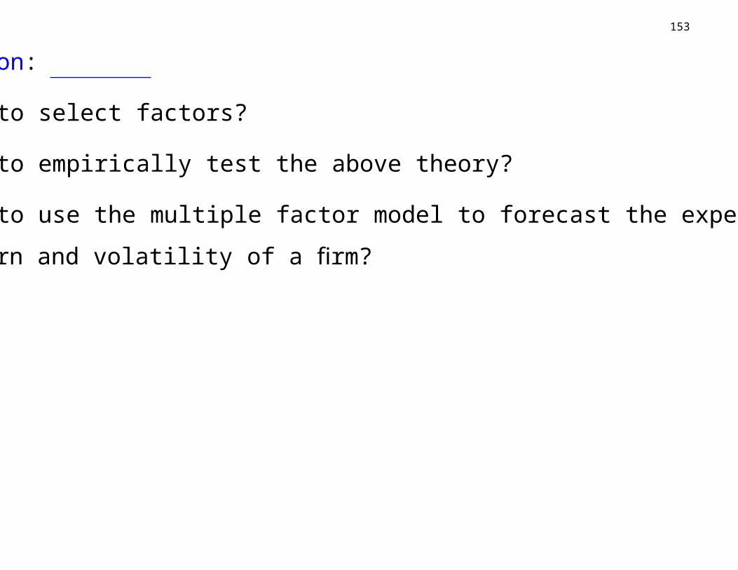
Question:

— How to select factors?

— How to empirically test the above theory?

— How to use the multiple factor model to forecast the expected

return and volatility of a firm?

154

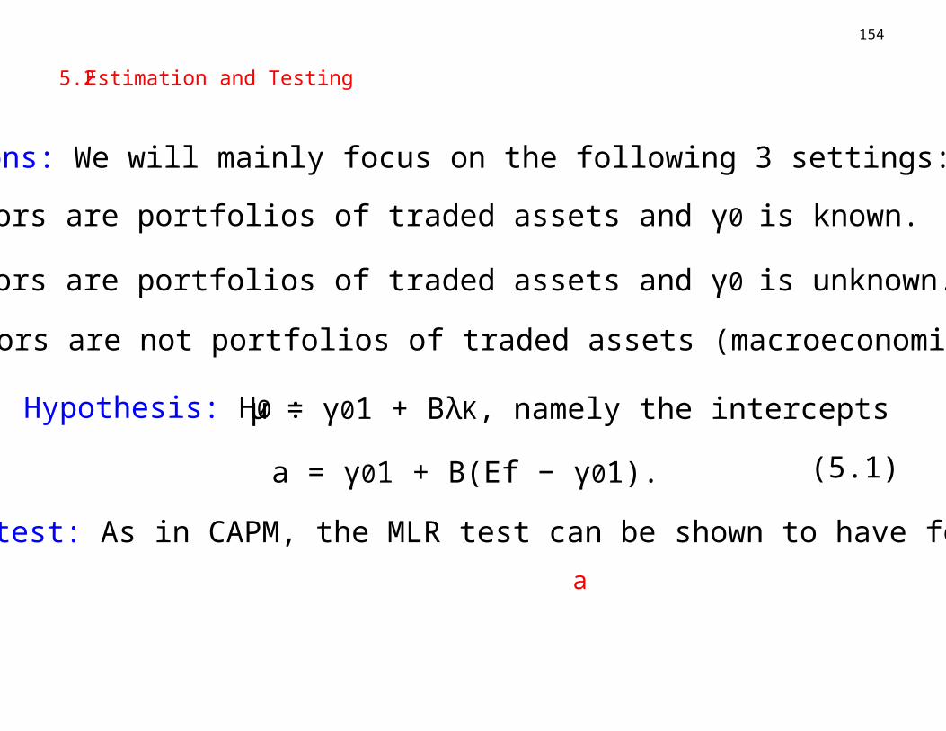
5.2 Estimation and Testing

Situations: We will mainly focus on the following 3 settings:

(a) Factors are portfolios of traded assets and γ0 is known.

(b) Factors are portfolios of traded assets and γ0 is unknown.

(c) Factors are not portfolios of traded assets (macroeconomic var).

Hypothesis: H0 : µ = γ01 + BλK, namely the intercepts

a = γ01 + B(Ef − γ01). (5.1)

MLR test: As in CAPM, the MLR test can be shown to have form

a

155

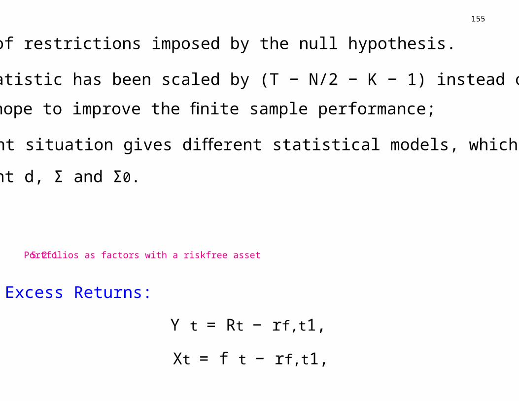
— d = # of restrictions imposed by the null hypothesis.

— the statistic has been scaled by (T − N/2 − K − 1) instead of T

in an hope to improve the finite sample performance;

— di erent situation gives di erent statistical models, which result inff ff

di erent d, Σ and Σff 0.

5.2.1 Portfolios as factors with a riskfree asset

Excess Returns:

Y t = Rt − rf,t1,

Xt = f t − rf,t1,

(Y t − Y¯ )(Xt − X)T (Xt − X)(Xt − X)T

a = Y¯ − BX,

156

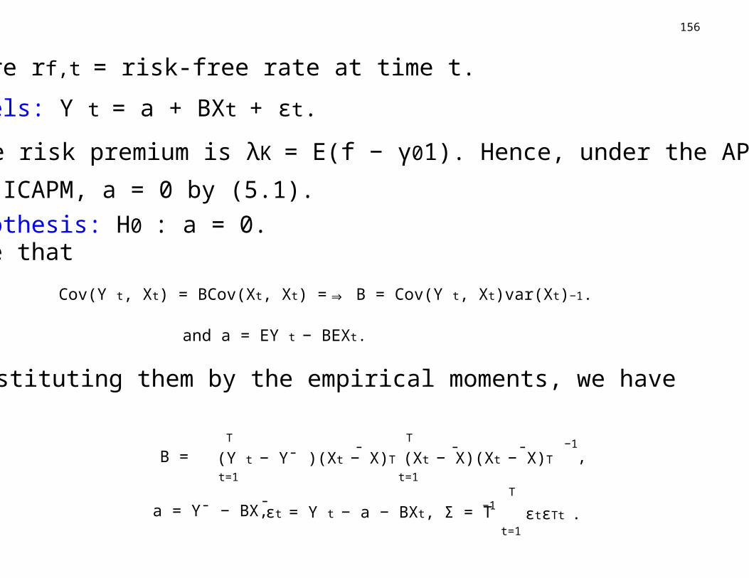
where rf,t = risk-free rate at time t.

Models: Y t = a + BXt + εt.

The risk premium is λK = E(f − γ01). Hence, under the APT

and ICAPM, a = 0 by (5.1).

Hypothesis: H0 : a = 0.Note that

Cov(Y t, Xt) = BCov(Xt, Xt) = B = Cov(Y ⇒ t, Xt)var(Xt)−1.

and a = EY t − BEXt.

Substituting them by the empirical moments, we haveMLE:

B =T

t=1

¯T

t=1

¯ ¯−1

,

¯ εt = Y t − a − BXt, Σ = T −1T

t=1

εtεTt .

tXt ][

157

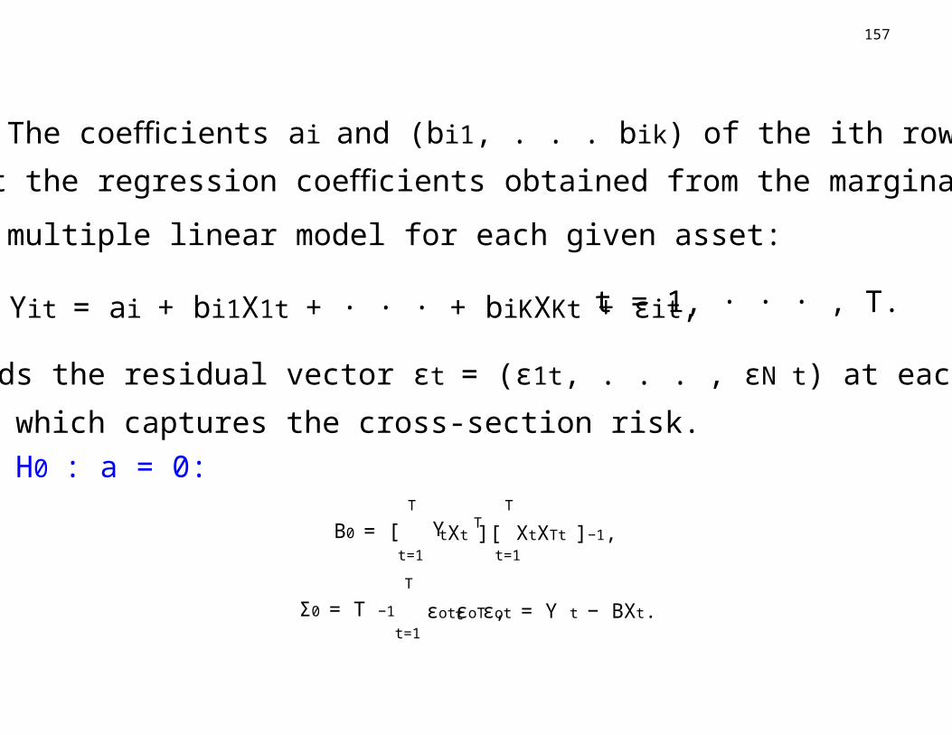
Remark: The coe cients affi i and (bi1, . . . bik) of the ith row of B

are just the regression coe cients obtained from the marginal models:ffiFit the multiple linear model for each given asset:

Yit = ai + bi1X1t + · · · + biKXKt + εit, t = 1, · · · , T.

This yields the residual vector εt = (ε1t, . . . , εN t) at each given time

period t, which captures the cross-section risk.

MLE under H0 : a = 0:

B0 = [T

t=1

Y TT

t=1

XtXTt ]−1,

Σ0 = T −1

T

t=1tεotεoT , εot = Y t − BXt.

¯ T −1[1 + X ΩK X]−1aT Σ−1a ∼0 FN,T −N −K .

158

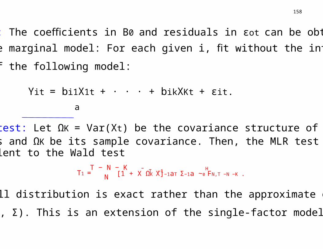
Remark: The coe cients in Bffi 0 and residuals in εot can be obtained

via the marginal model: For each given i, fit without the intercept

term of the following model:

Yit = bi1X1t + · · · + bikXKt + εit.

a

Exact test: Let ΩK = Var(Xt) be the covariance structure of Kfactors and ΩK be its sample covariance. Then, the MLR test isequivalent to the Wald test

T1 =T − N − K

NH

This null distribution is exact rather than the approximate one if

ε N (∼ 0, Σ). This is an extension of the single-factor model.

159

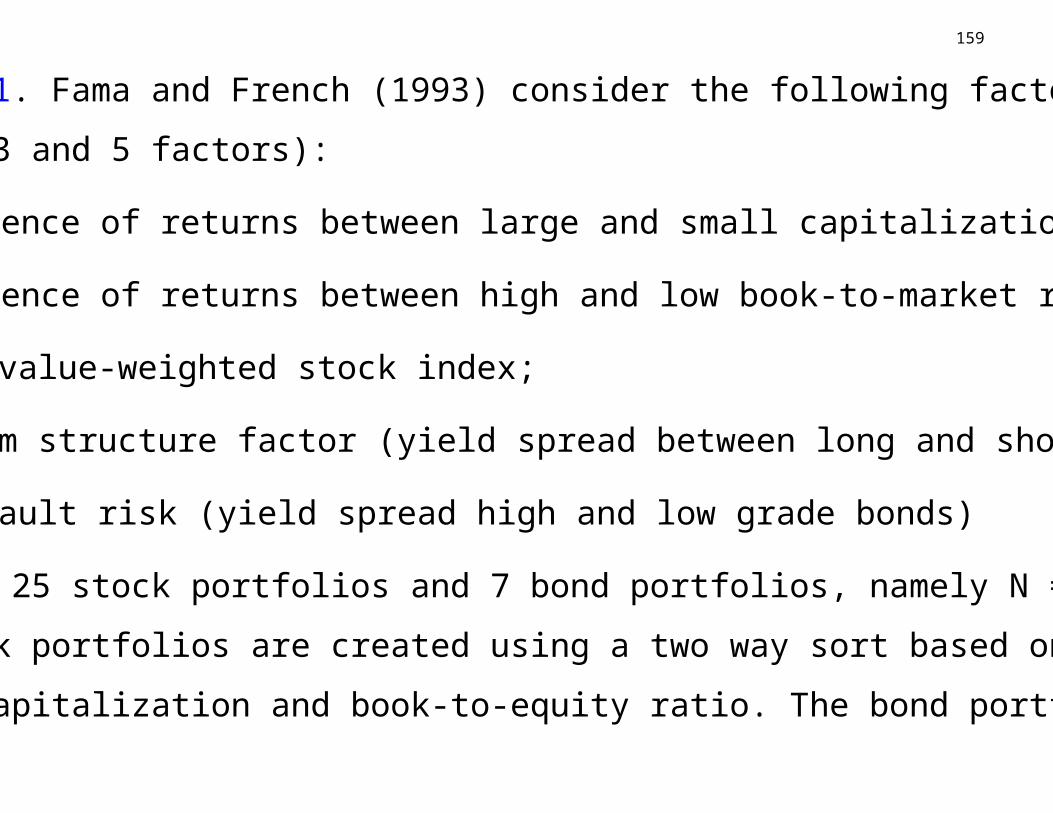
Example 1. Fama and French (1993) consider the following factors

(K = 2, 3 and 5 factors):

1. di erence of returns between large and small capitalization;ff

2. di erence of returns between high and low book-to-market ratios;ff

3. CRSP value-weighted stock index;

4. a term structure factor (yield spread between long and short bonds);

5. a default risk (yield spread high and low grade bonds)

They use 25 stock portfolios and 7 bond portfolios, namely N = 32.

The stock portfolios are created using a two way sort based on the

market capitalization and book-to-equity ratio. The bond portfolios

160

include five US government and two corporate bound portfolios. The

period of study is 1963/07–1991/12, namely T = 354. The P-values

are summarized as follows based on the test statistic T1.

Table 5.1: Summary of testing results using the exact F-test

K 2 3 5

P-value 0.010 0.039 0.025

Fama and Fama find

— some improvement going from two factors to five factors;

— three factors are necessary when testing portfolio consisting only

of stocks;

— five factors when bond portfolio is included.

161

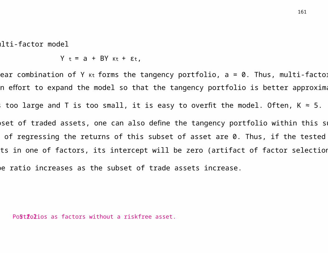
Remarks:∗

1. In the multi-factor model

Y t = a + BY Kt + εt,

when a linear combination of Y Kt forms the tangency portfolio, a = 0. Thus, multi-factor

model is an e ort to expand the model so that the tangency portfolio is better approximated.ff

2. When K is too large and T is too small, it is easy to overfit the model. Often, K ≈ 5.

3. For a subset of traded assets, one can also define the tangency portfolio within this subset. The

intercepts of regressing the returns of this subset of asset are 0. Thus, if the tested assets have

high weights in one of factors, its intercept will be zero (artifact of factor selection).

4. The Sharpe ratio increases as the subset of trade assets increase.

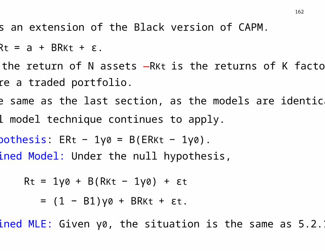
5.2.2 Portfolios as factors without a riskfree asset.

162

This is an extension of the Black version of CAPM.

Model: Rt = a + BRKt + ε.

— Rt is the return of N assets —RKt is the returns of K factors,

which are a traded portfolio.

MLE: The same as the last section, as the models are identical. The

marginal model technique continues to apply.

Null hypothesis: ERt − 1γ0 = B(ERKt − 1γ0).

Constrained Model: Under the null hypothesis,

Rt = 1γ0 + B(RKt − 1γ0) + εt

= (1 − B1)γ0 + BRKt + εt.

Constrained MLE: Given γ0, the situation is the same as 5.2.1

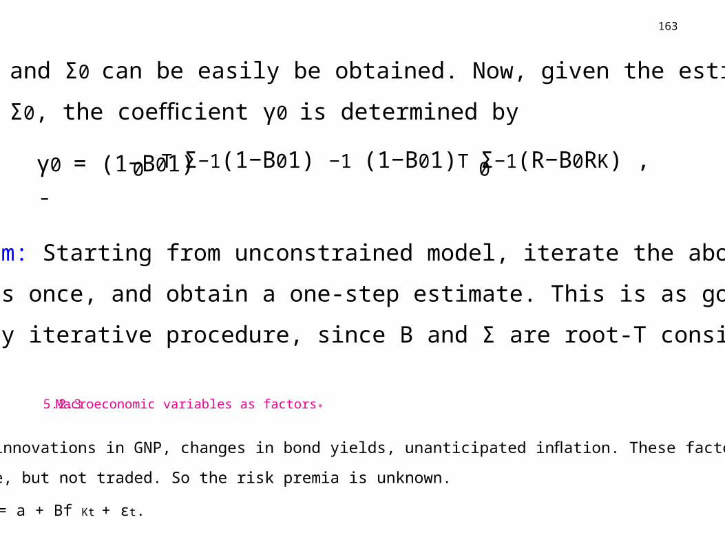
T Σ−1(1−B01) −1 (1−B01)T Σ−1(R−B0RK) ,

163

and B0 and Σ0 can be easily be obtained. Now, given the estimated

B0 and Σ0, the coe cient γffi 0 is determined by

γ0 = (1−B01) 0 0

¯ ¯

Algorithm: Starting from unconstrained model, iterate the above

equations once, and obtain a one-step estimate. This is as good as

the fully iterative procedure, since B and Σ are root-T consistent.

5.2.3 Macroeconomic variables as factors∗

Example: innovations in GNP, changes in bond yields, unanticipated inflation. These factors are

observable, but not traded. So the risk premia is unknown.

Model: Rt = a + Bf Kt + εt.

164

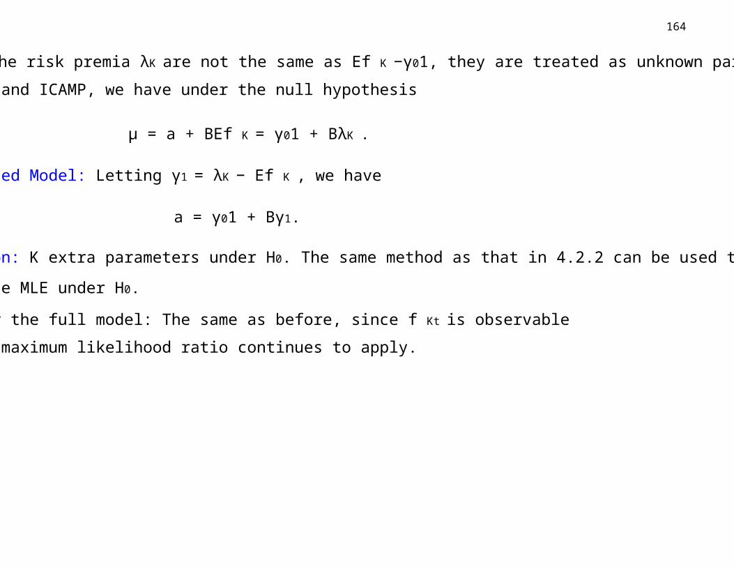
Since the risk premia λK are not the same as Ef K −γ01, they are treated as unknown parameters.

From APT and ICAMP, we have under the null hypothesis

µ = a + BEf K = γ01 + BλK .

Constrained Model: Letting γ1 = λK − Ef K , we have

a = γ01 + Bγ1.

Comparison: K extra parameters under H0. The same method as that in 4.2.2 can be used to

obtain the MLE under H0.

MLE under the full model: The same as before, since f Kt is observable

MLR: The maximum likelihood ratio continues to apply.

λk = X = T −1

165

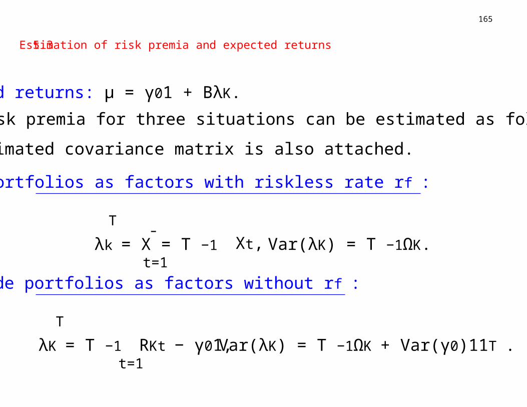
5.3 Estimation of risk premia and expected returns

¯

Expected returns: µ = γ01 + BλK.

The risk premia for three situations can be estimated as follows.

The estimated covariance matrix is also attached.

Trade portfolios as factors with riskless rate rf :

T

Xt, Var(λK) = T −1ΩK.

λK = T −1

t=1

Trade portfolios as factors without rf :

T

t=1RKt − γ01, Var(λK) = T −1ΩK + Var(γ0)11T .

166

λK = T −1

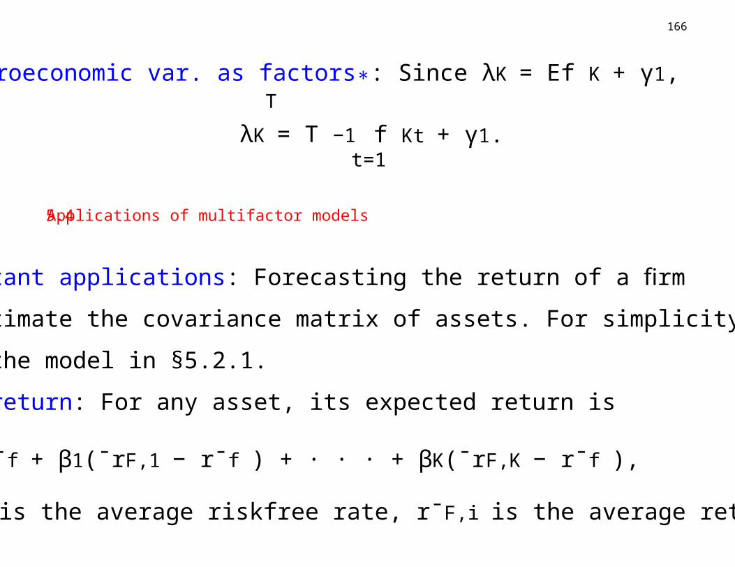
Macroeconomic var. as factors∗: Since λK = Ef K + γ1,T

t=1f Kt + γ1.

5.4 Applications of multifactor models

Two important applications: Forecasting the return of a firm

and to estimate the covariance matrix of assets. For simplicity, we

consider the model in §5.2.1.

Forecast return: For any asset, its expected return is

r¯f + β1(¯rF,1 − r¯f ) + · · · + βK(¯rF,K − r¯f ),

where r¯f is the average riskfree rate, r¯F,i is the average return of the

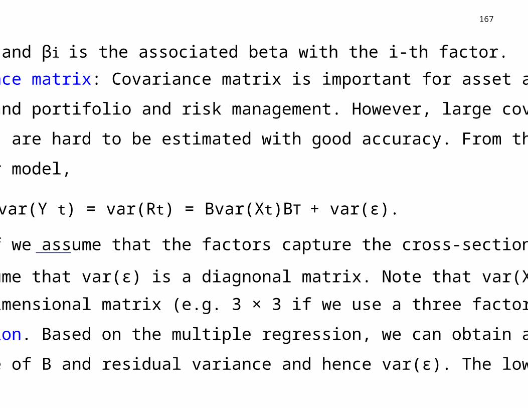
167

factor, and βi is the associated beta with the i-th factor.

Covariance matrix: Covariance matrix is important for asset allo-

cation and portifolio and risk management. However, large covariance

matrices are hard to be estimated with good accuracy. From the mul-

tifactor model,

var(Y t) = var(Rt) = Bvar(Xt)BT + var(ε).

Idea: If we assume that the factors capture the cross-section risk, we

may assume that var(ε) is a diagnonal matrix. Note that var(Xt) is

a low-dimensional matrix (e.g. 3 × 3 if we use a three factor model).

Estimation. Based on the multiple regression, we can obtain an

estimate of B and residual variance and hence var(ε). The low-

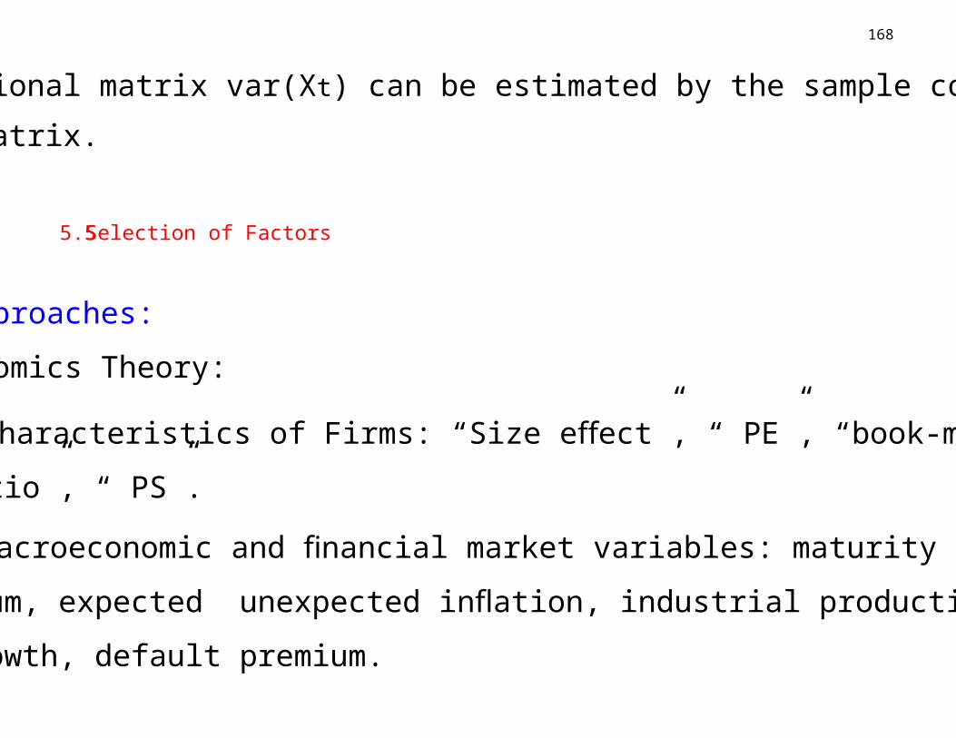
168

dimensional matrix var(Xt) can be estimated by the sample covari-

ance matrix.

5.5 Selection of Factors

Two approaches:

— Economics Theory:

(a) Characteristics of Firms: “Size e ect”, “ PE”, “book-marketffratio”, “ PS”.

(b) macroeconomic and financial market variables: maturity pre-

mium, expected unexpected inflation, industrial production

growth, default premium.

= B B + Σ, B = ΩK B.

169

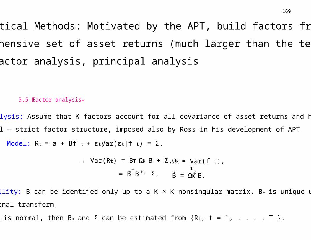
— Statistical Methods: Motivated by the APT, build factors from a

comprehensive set of asset returns (much larger than the test sets),

e.g. factor analysis, principal analysis

5.5.1 Factor analysis∗

Factor analysis: Assume that K factors account for all covariance of asset returns and hence Σ

is diagonal — strict factor structure, imposed also by Ross in his development of APT.

Model: Rt = a + Bf t + εt, Var(εt|f t) = Σ.

⇒ Var(Rt) = BT ΩK B + Σ,

∗T ∗

ΩK = Var(f t),1

∗ 2

Identifiability: B can be identified only up to a K × K nonsingular matrix. B ∗ is unique up to

an orthogonal transform.

MLE: If εt is normal, then B ∗ and Σ can be estimated from Rt, t = 1, . . . , T .

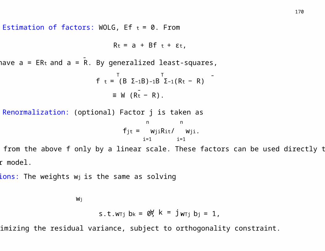
we have a = ERt and a = R. By generalized least-squares,

¯f t = (B Σ−1B)−1B Σ−1(Rt − R)

≡ W (Rt − R).

170

Estimation of factors: WOLG, Ef t = 0. From

Rt = a + Bf t + εt,

¯

T T

¯

Renormalization: (optional) Factor j is taken as

fjt =n

i=1

wjiRit/n

i=1

wji.

This di ers from the above f only by a linear scale. These factors can be used directly to fit aff

multi-factor model.

Interpretations: The weights wj is the same as solving

wj

s.t.wTj bk = 0, ∀ k = j, wTj bj = 1,

i.e. minimizing the residual variance, subject to orthogonality constraint.

171

Proof: Let ej be the K-dimensional unit vector with one at the jth position. Then, the side

condition can be written asT

B wj = ej.

By the Lagrange multiplier method, we minimize

T

Taking derivative and setting it to zero

Σwj − Bλ = 0 or wj = Σ−1Bλ.

Now, using the constraintT T

T

T

T T

The converse follow obvious from the above derivation:

TB wj = ej.

172

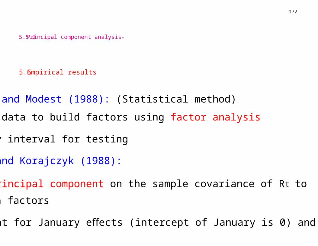
5.5.2

5.6

Principal component analysis∗

Empirical results

Lehmann and Modest (1988): (Statistical method)

— daily data to build factors using factor analysis

— weekly interval for testing

Connor and Korajczyk (1988):

— use principal component on the sample covariance of Rt to

obtain factors

— account for January e ects (intercept of January is 0) and non Jan.ff

173

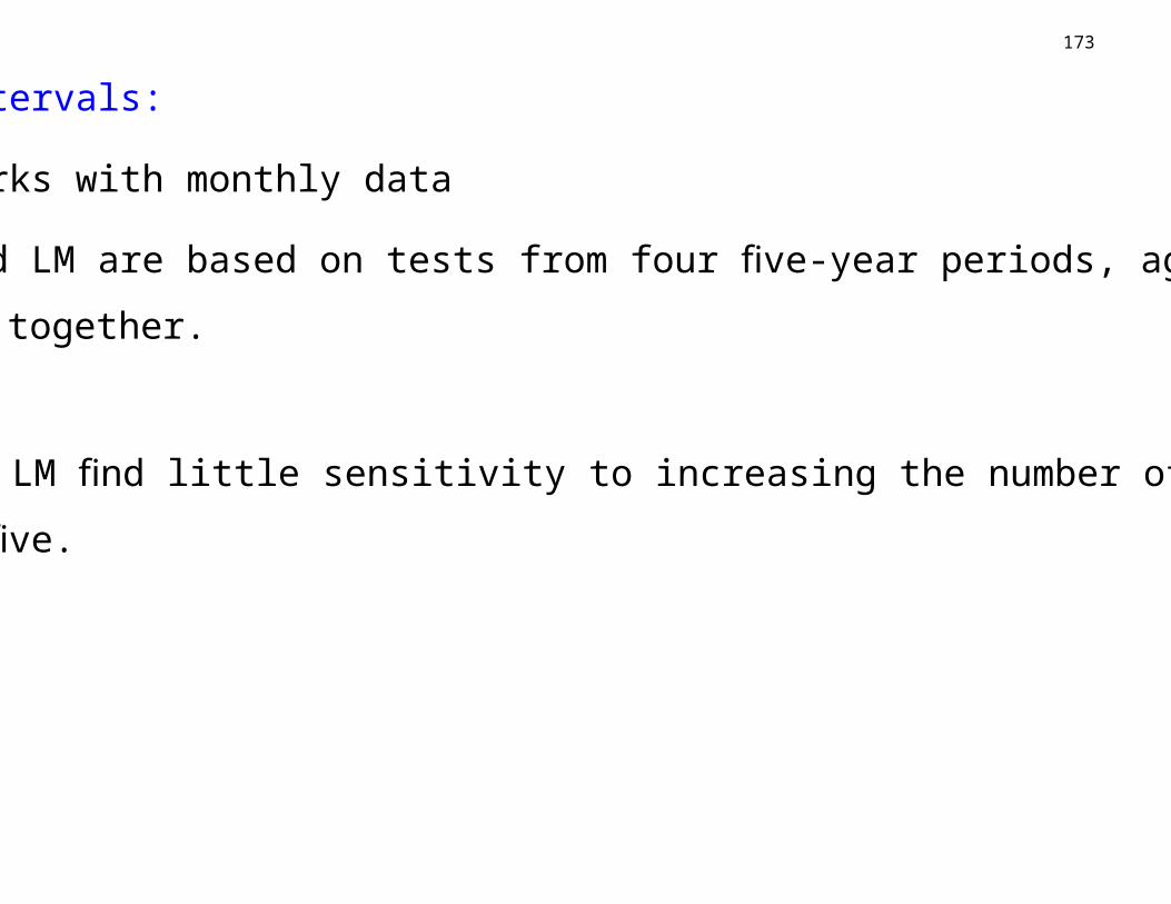
Test intervals:

— CK works with monthly data

— CK and LM are based on tests from four five-year periods, aggre-

gated together.

Results:

CK and LM find little sensitivity to increasing the number of factors

beyond five.

174

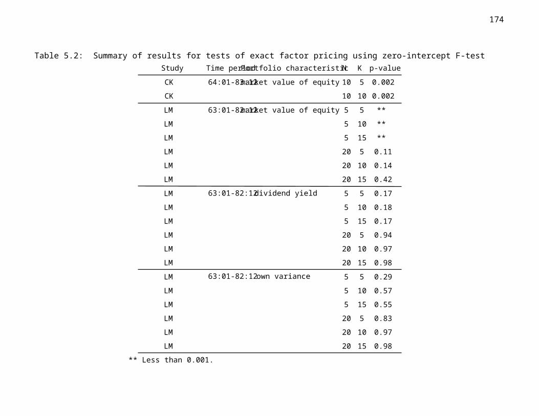
Table 5.2: Summary of results for tests of exact factor pricing using zero-intercept F-test

Time period

64:01-83:12

63:01-82:12

63:01-82:12

63:01-82:12

Portfolio characteristic

market value of equity

market value of equity

dividend yield

own variance

Study

CK

CK

LM

LM

LM

LM

LM

LM

LM

LM

LM

LM

LM

LM

LM

LM

LM

LM

LM

LM

N

10

10

5

5

5

20

20

20

5

5

5

20

20

20

5

5

5

20

20

20

K

5

10

5

10

15

5

10

15

5

10

15

5

10

15

5

10

15

5

10

15

p-value

0.002

0.002

**

**

**

0.11

0.14

0.42

0.17

0.18

0.17

0.94

0.97

0.98

0.29

0.57

0.55

0.83

0.97

0.98

** Less than 0.001.