Chapter 5:

Consumer Choices and Economic

Behavior

Key Topics

1. The budget constrainta. Definition, equation, graph, opportunity cost

b. Impact of ΔI, ΔPx, ΔPy

2. Utilitya. Total and marginal

b. Indifference curve: definition, slope

c. Utility maximization

Key Topics

3. Downward-sloping demand factorsa. Diminishing marginal utility

b. Income effect

c. Substitution effect

4. Other consumer decisionsa. Work or leisure

b. Save or borrow

Questions

1. What does it mean if you have a ‘budget constraint’?

2. How can your attainable consumption choices be shown mathematically and graphically?

Budget Constraint

The maximum Q combinations of goods

that can be purchased given one’s income and the prices of the goods.

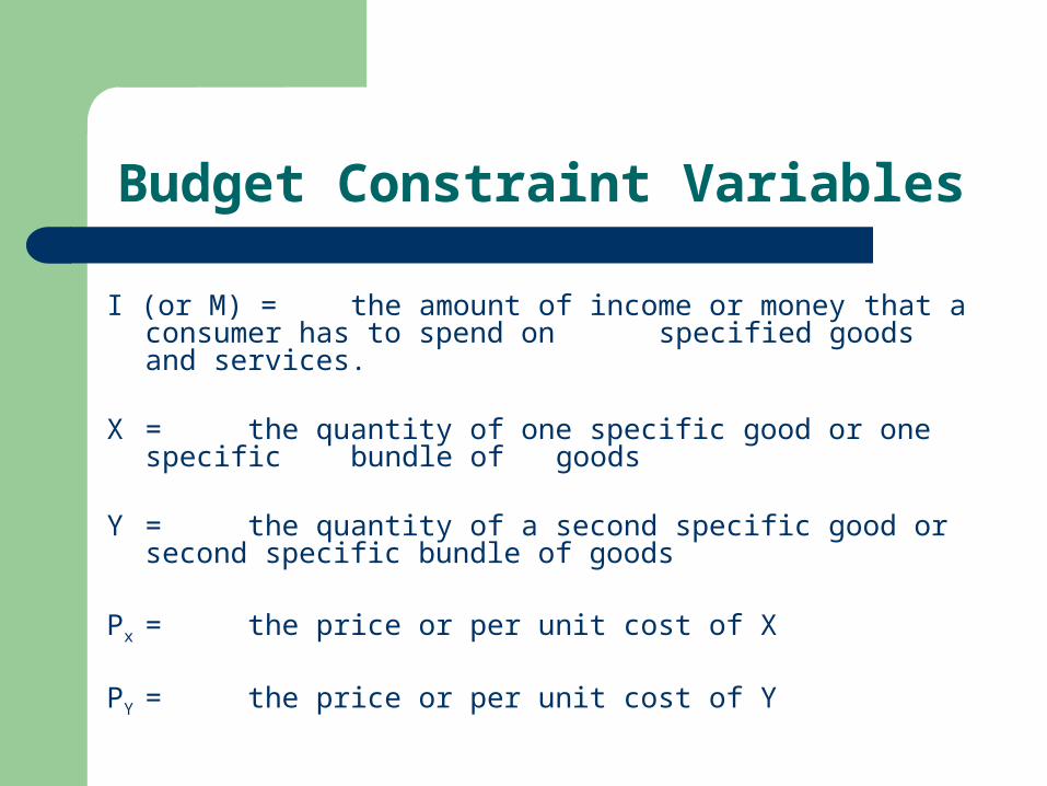
Budget Constraint Variables

I (or M) = the amount of income or money that a consumer has to spend on

specified goods and services.

X = the quantity of one specific good or one specific bundle of goods

Y = the quantity of a second specific good or second specific bundle of goods

Px = the price or per unit cost of X

PY = the price or per unit cost of Y

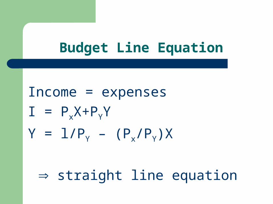
Budget Line Equation

Income = expenses

I = PxX+PYY

Y = l/PY – (Px/PY)X

straight line equation

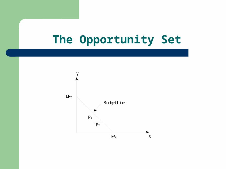
The Opportunity Set

Y

I/PYI/PY

Budget Line

PX

PY

I/PX X

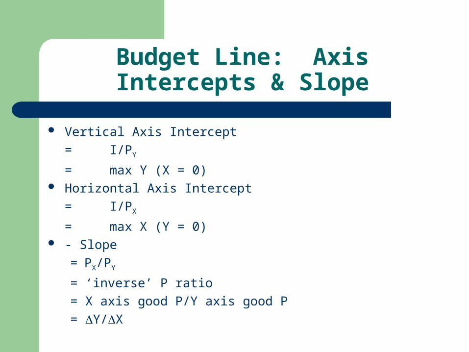
Budget Line: Axis Intercepts & Slope

Vertical Axis Intercept

= I/PY

= max Y (X = 0) Horizontal Axis Intercept

= I/PX

= max X (Y = 0) - Slope

= PX/PY

= ‘inverse’ P ratio

= X axis good P/Y axis good P

= Y/X

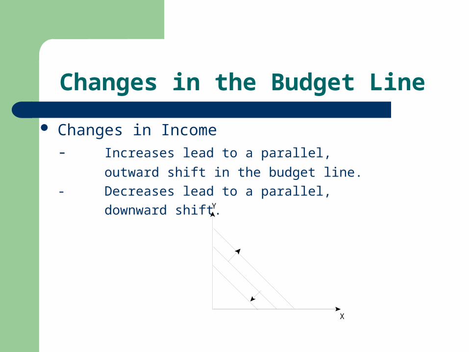
Changes in the Budget Line

Changes in Income

- Increases lead to a parallel,

outward shift in the budget line.

- Decreases lead to a parallel,

downward shift. Y

X

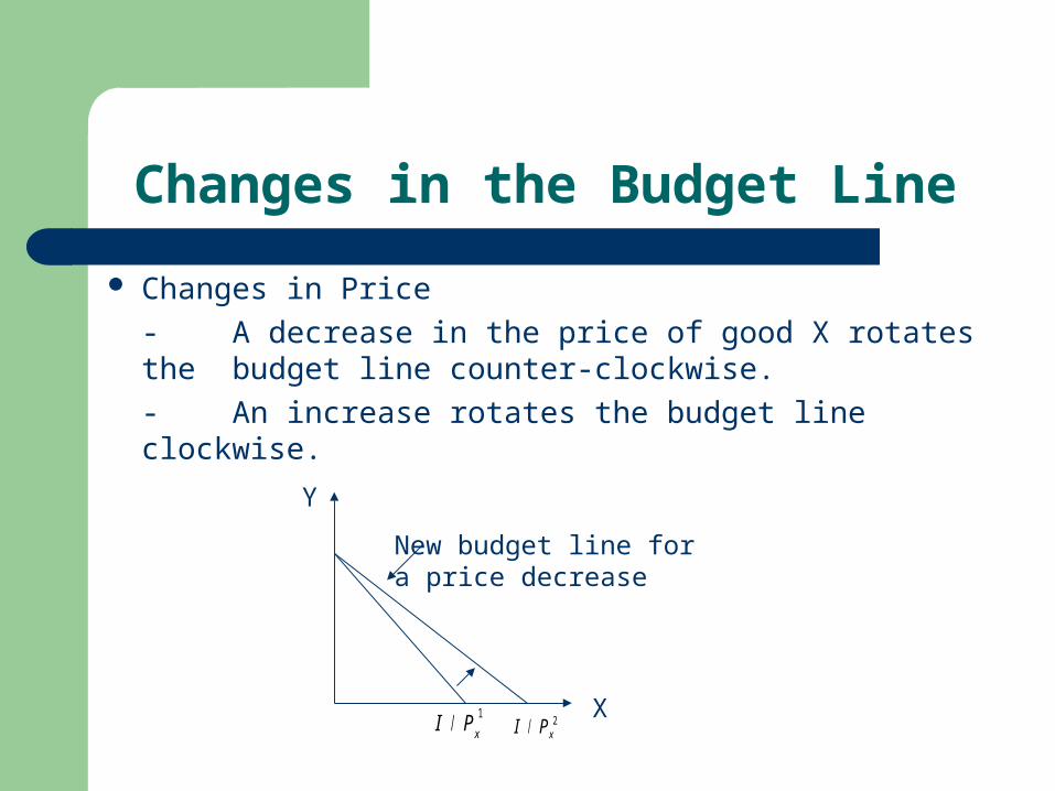
Changes in the Budget Line

Changes in Price

- A decrease in the price of good X rotates the budget line counter-clockwise.

- An increase rotates the budget line clockwise.

I Px

/1

New budget line fora price decrease

X

Y

I Px/ 2

Q. What Are Your Preferences?

LunchA: 1 drink, 1 pizza sliceB: 1 drink, 2 pizza slicesC: 2 drinks, 1 pizza slice

EntertainmentA: 1 movie, 1 dinnerB: 1 movie, 2 dinnersC: 2 movies, 1 dinnerFor each, indicate which of the following you prefer:

A vs B, B vs C, or A vs C

Utility Concepts

Utility:satisfaction received from consuming goods

Cardinal utility:satisfaction levels that can be measured or specified with numbers (units = ‘utils’)

Ordinal utility:satisfaction levels that can be ordered or ranked

Marginal utility:the additional utility received per unit of additional unit of an item consumed (ΔU/ ΔX)

Utility Assumptions

1. Complete (or continuous) can rank all bundles of goods

2. Consistent (or transitive) preference orderings are logical and consistent

3. Consumptive (nonsatiation) more of a ‘normal’ good is preferred to less

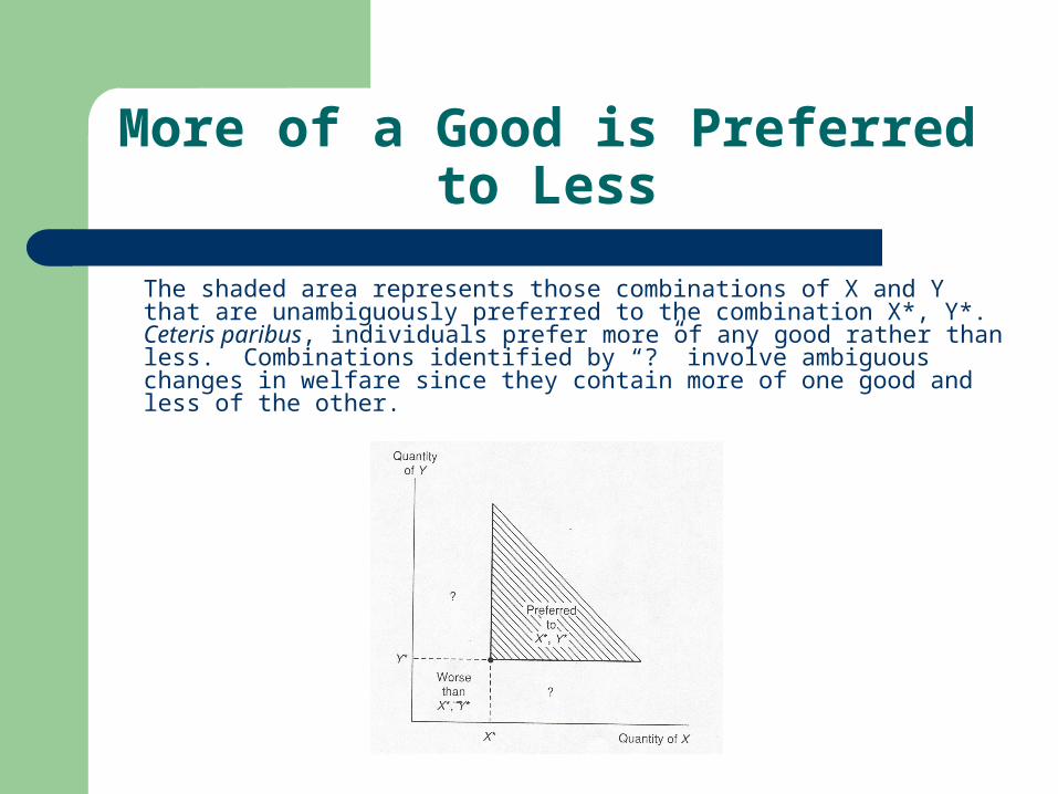
More of a Good is Preferred to Less

The shaded area represents those combinations of X and Y that are unambiguously preferred to the combination X*, Y*. Ceteris paribus, individuals prefer more of any good rather than less. Combinations identified by “?” involve ambiguous changes in welfare since they contain more of one good and less of the other.

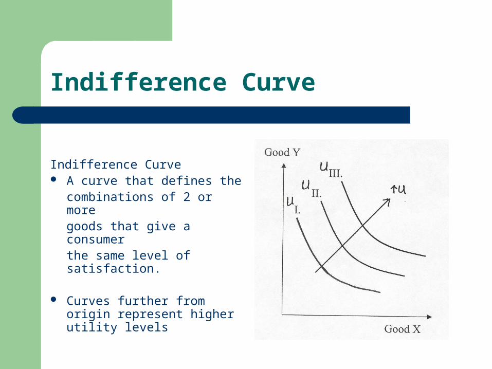
Indifference Curve

Indifference Curve A curve that defines the

combinations of 2 or more goods that give a consumer the same level of satisfaction.

Curves further from origin represent higher utility levels

A ‘bad’ good, or an economic ‘bad’ is an item that a consumer does not like or enjoy, which means their total satisfaction level is lower the more of the item they have. This also means the marginal utility of the item is negative.

MRS & MU

MRS= - slope of indifference curve= -Y/ X= the rate at which a consumer is willing to

exchange Y for 1more (or less) unit of XU = 0 along given indiff curve

= MUx(X)+MUY(Y) = 0

= - Y/ X = MUx/MUY

= - slope = inverse MU ratio

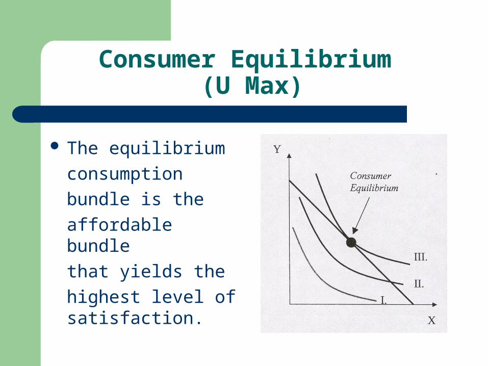
Consumer Equilibrium (U Max)

The equilibrium

consumption

bundle is the

affordable bundle

that yields the

highest level of satisfaction.

Equal Slopes Condition (for consumer equilibrium)

MUX/MUY = PX/PY

MUX/PX = MUY/PY

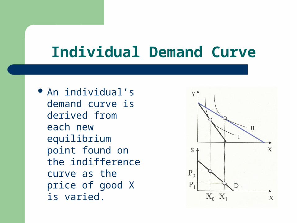
Individual Demand Curve

An individual’s demand curve is derived from each new equilibrium point found on the indifference curve as the price of good X is varied.

Diminishing Marginal Utility

The law of diminishing marginal utility:

The more of one good consumed in a given period, the less satisfaction (utility) generated by consuming each additional (marginal) unit of the same good.

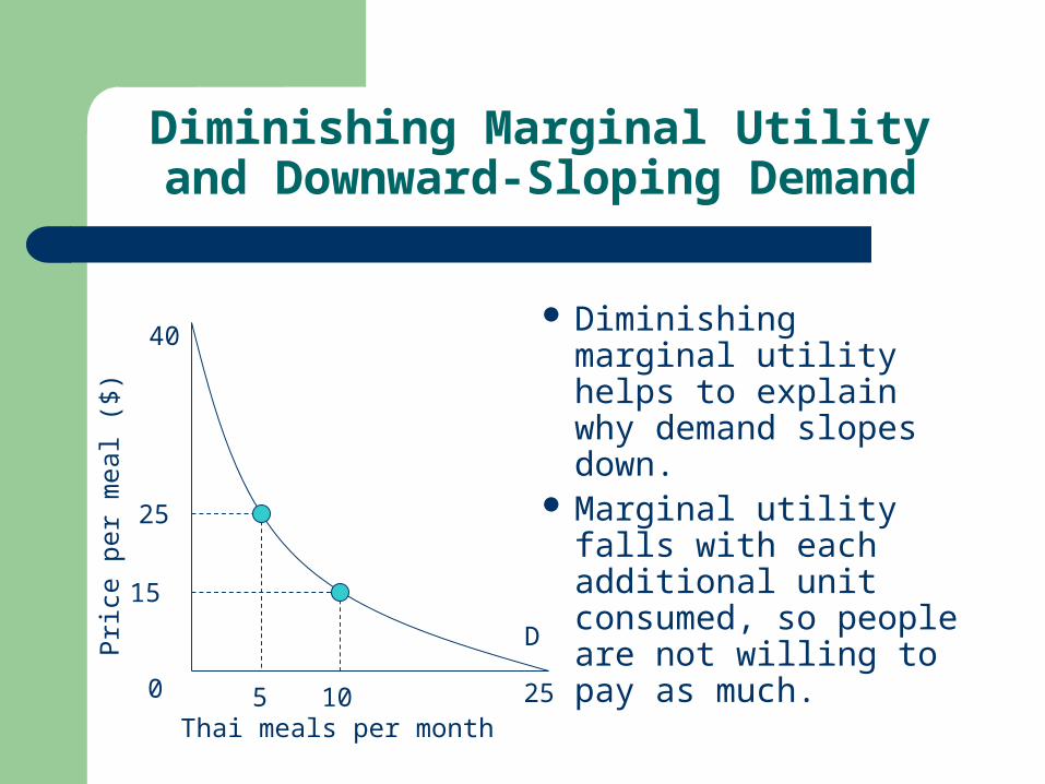
Diminishing Marginal Utility and Downward-Sloping Demand

Diminishing marginal utility helps to explain why demand slopes down.

Marginal utility falls with each additional unit consumed, so people are not willing to pay as much.

40

25

15

0 5 10 25

D

Thai meals per month

Pric

e pe

r m

eal (

$)

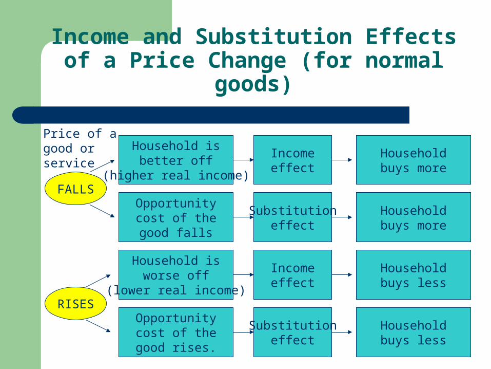
Income and Substitution Effects of a Price Change (for normal goods)

Household isbetter off

(higher real income)

Opportunitycost of thegood falls

Household isworse off

(lower real income)

Opportunitycost of thegood rises.

Incomeeffect

Substitutioneffect

Incomeeffect

Substitutioneffect

Householdbuys more

FALLS

RISES

Householdbuys more

Householdbuys less

Householdbuys less

Price of agood or service

Household Choices in Labor Markets

As in output markets, households face constrained choices in input markets. They must decide:

1. Whether to work2. How much to work3. What kind of a job to work atThese decisions are affected by:1. The availability of jobs2. Market wage rates3. The skill possessed by the household

The Price of Leisure

W = wage rate

= the price (or the opportunity cost or lost benefits) of either

unpaid work or leisure.

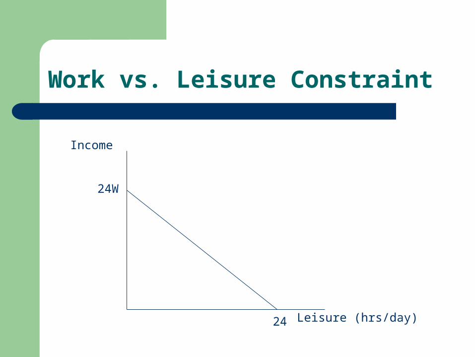
Work vs. Leisure Constraint

24W

24 Leisure (hrs/day)

Income

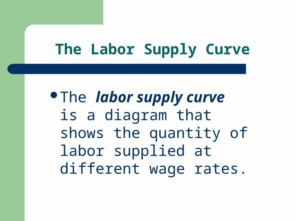
The Labor Supply Curve

The labor supply curve is a diagram that shows the quantity of labor supplied at different wage rates.

Saving and Borrowing: Present Versus Future Consumption

Households can use present income to finance future spending (i.e., save), or they can use future funds to finance present spending (i.e., borrow).

In deciding how much to save and how much to spend today, interest rates define the opportunity cost of present consumption in terms of foregone future consumption.

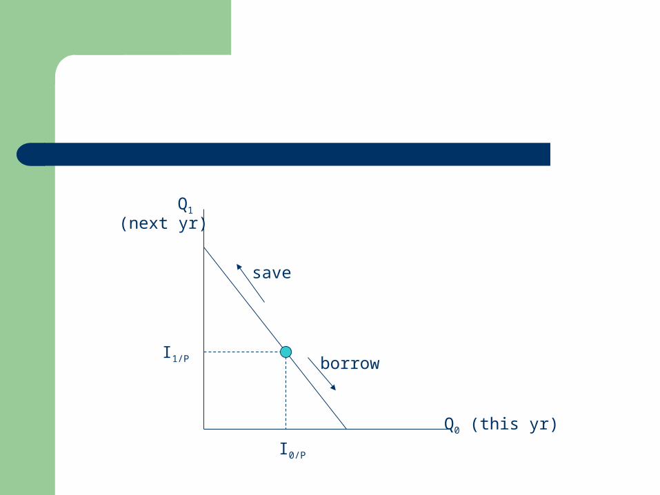
borrow

save

Q1

(next yr)

I1/P

I0/P

Q0 (this yr)