Chapter 4 Numerical Techniques for Parabolic, Elliptic ... · Page 4-1 Chapter 4 Numerical...
74
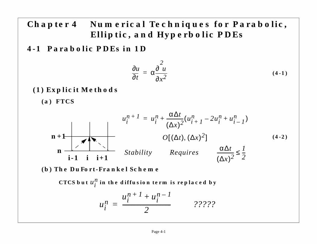
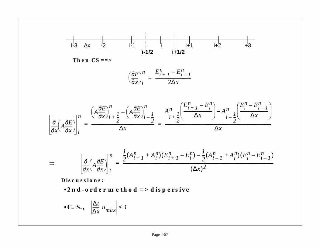
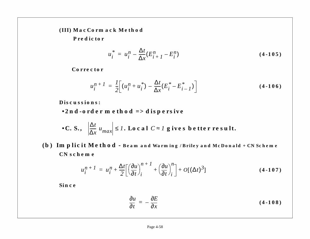
Page 4-1 Chapter 4 Numerical Techniques for Parabolic, Elliptic, and Hyperbolic PDEs 4-1 Parabolic PDEs in 1D (4-1) (1) Explicit Methods (a) FTCS (4-2) (b) The DuFort-Frankel Scheme CTCS but in the diffusion term is replaced by t ∂ ∂u α x 2 2 ∂ ∂ u = u i n 1 + u i n α∆ t ∆ x ( ) 2 -------------- u i 1 + n 2u i n – u i 1 – n + ( ) + = O ∆ t ( ) ∆ x ( ) 2 , [ ] Stability Requires α∆ t ∆ x ( ) 2 -------------- 1 2 -- ≤ i-1 i i+1 n n+1 u i n u i n u i n 1 + u i n 1 – + 2 --------------------------------- = ?????
Transcript of Chapter 4 Numerical Techniques for Parabolic, Elliptic ... · Page 4-1 Chapter 4 Numerical...
r Parabolic,DEs
(4-1)
(4-2)
ui 1–n+ )
∆ t
x)2---------
12---≤
Page 4-1
Chapter 4 Numerical Techniques foElliptic, and Hyperbolic P
4-1 Parabolic PDEs in 1D
(1) Explicit Methods
(a) FTCS
(b) The DuFort-Frankel Scheme
CTCS but in the diffusion term is replaced by
t∂∂u α
x2
2
∂∂ u
=
uin 1+ ui
n α∆ t
∆x( )2-------------- ui 1+
n 2uin–(+=
O ∆t( ) ∆x( )2,[ ]
Stability Requiresα∆(
-----i-1 i i+1
n
n+1
uin
uin
uin 1+ ui
n 1–+
2---------------------------------= ?????
(4-3)
(4-4)
called time linear extrapolation?
t)] ∆t( ) O ∆t( )2[ ]+
)2]
1-----
1+ ui 1–n+ )
Page 4-2
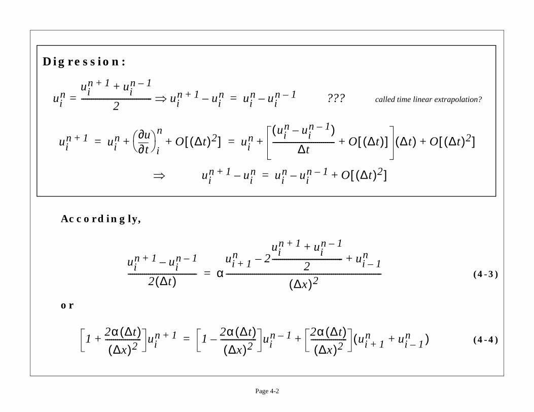
Digression:
Accordingly,
or
uin
uin 1+ ui
n 1–+
2-----------------------------------= ui
n 1+ uin–⇒ ui
n uin 1––= ???
uin 1+ ui
nt∂∂u
i
nO ∆t( )2[ ]+ + ui
nui
n uin 1––( )
∆t------------------------------- O ∆([++= =
⇒ uin 1+ ui
n– uin ui
n 1–– O ∆t([+=
uin 1+ ui
n 1––
2 ∆t( )---------------------------------- α
ui 1+n 2
uin 1+ ui
n 1–+
2-----------------------------------– ui –
n+
∆x( )2------------------------------------------------------------------------=
12α ∆ t( )∆x( )2
------------------+ uin 1+ 1
2α ∆ t( )∆x( )2
------------------– uin 1– 2α ∆ t( )
∆x( )2------------------ ui
n(+=
(4-5)
e rate, such that
ol. to start with and 2
(4-3)/(4-4) gives
x)2 O ∆x( )4[ ]+t
n
tx
---- 0⇒
αt2
2
∂∂ u
A Hyp. Eq.=
Page 4-3
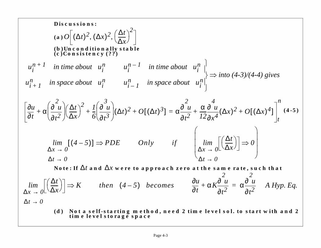
Discussions:
(a)
(b)Unconditionally stable(c)Consistency (??)
Note: If and were to approach zero at the sam
(d) Not a self-starting method, need 2 time level stime level storage space
O ∆t( )2 ∆x( )2 ∆t∆x------ 2
, ,
uin 1+ in time about ui
n uin 1– in time about ui
n
ui 1+n in space about ui
n ui 1–n in space about ui
n
into⇒
t∂∂u α
t2
2
∂∂ u
∆t
∆x------ 2 1
6---
t3
3
∂∂ u
∆t( )2 O ∆t( )3[ ]+ ++ αt2
2
∂∂ u α
12------
x4
4
∂∂ u ∆(+=
4 5–( )[ ]∆x 0→∆t 0→
lim PDE⇒ Only if∆∆--
∆x 0→∆t 0→
lim
∆t ∆x
∆t∆x------
∆x 0→∆t 0→
lim K⇒ then 4 5–( ) becomest∂∂u αK
t2
2
∂∂ u
+
icit Scheme)
(4-6)
(4-7)ui
n 1+ uin–
β 1≤ ≤
∆t( )2[ ]
Page 4-4
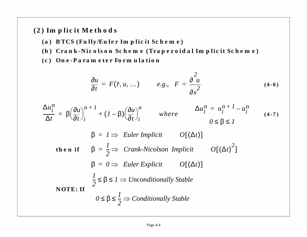
(2) Implicit Methods
(a) BTCS (Fully/Euler Implicit Scheme)
(b) Crank-Nicolson Scheme (Trapezoidal Impl
(c) One-Parameter Formulation
then if
NOTE: If
t∂∂u
F r u …, ,( )= e.g., Fx
2
2
∂
∂ u=
∆uin
∆t---------- β
t∂∂u
i
n 1+1 β–( )
t∂∂u
i
n+= where
∆uin =
0
β 1 Euler Implicit⇒= O ∆t( )[ ]
β 12--- Crank-Nicolson Implicit⇒= O
β 0 Euler Explicit⇒= O ∆t( )[ ]12--- β 1 Unconditionally Stable⇒≤ ≤
0 β 12--- Conditionally Stable⇒≤ ≤
(4-8)
(4-9)
er/nonlinear in u):
∂∂
linearization, e.g.,
nO ∆t( )2[ ]+
E Au∂∂E
and Bu∂∂F
= =
n Bn∆un O ∆t( )2[ ]+ +
Page 4-5
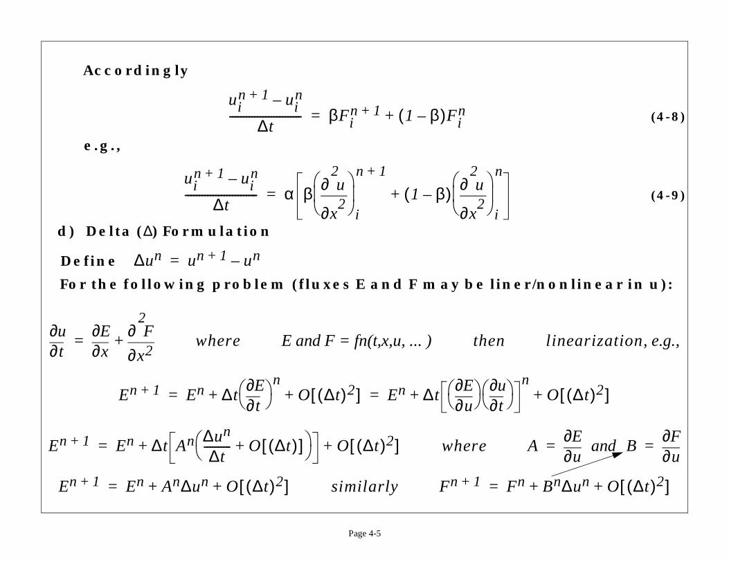
Accordingly
e.g.,
d) Delta (∆) Formulation
Define
For the following problem (fluxes E and F may be lin
uin 1+ ui
n–
∆t-------------------------- βFi
n 1+ 1 β–( )Fin+=
uin 1+ ui
n–
∆t-------------------------- α β
x2
2
∂
∂ u
i
n 1+
1 β–( )x
2
2
∂
∂ u
i
n
+=
∆un un 1+ un–=
tu
x∂∂E
x2
2
∂∂ F
+= where E and F = fn(t,x,u, ... ) then
En 1+ En ∆tt∂∂E n
O ∆t( )2[ ]+ + En ∆tu∂∂E
t∂∂u += =
n 1+ En ∆t An ∆un
∆t---------- O ∆t( )[ ]+ O ∆t( )2[ ]+ += where
En 1+ En An∆un O ∆t( )2[ ]+ += similarly Fn 1+ F=
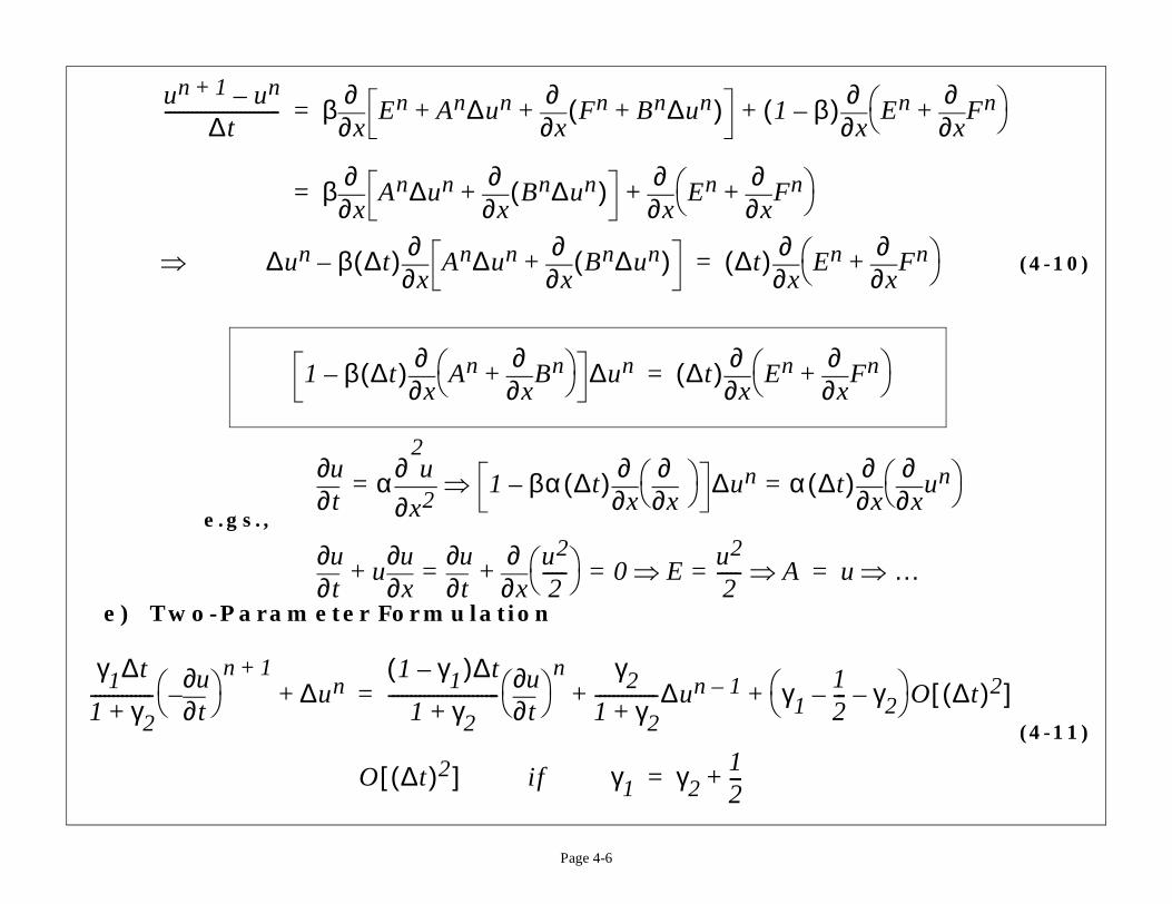
(4-10)
(4-11)
x∂∂
Enx∂∂
Fn+
x∂∂
Fn+
Fn
)x∂∂
x∂∂
un
u …⇒
γ2– O ∆t( )2[ ]
Page 4-6
e.gs.,
e) Two-Parameter Formulation
un 1+ un–∆t
-------------------------- βx∂∂
En An∆unx∂∂
Fn Bn∆un+( )+ + 1 β–( )+=
βx∂∂
An∆unx∂∂
Bn∆un( )+x∂∂
Enx∂∂
Fn+ +=
⇒ ∆un β ∆t( )x∂∂
An∆unx∂∂
Bn∆un( )+– ∆t( )x∂∂
En=
1 β ∆t( )x∂∂
Anx∂∂
Bn+ – ∆un ∆t( )
x∂∂
Enx∂∂
+=
t∂∂u α
x2
2
∂∂ u
= 1 βα ∆t( )x∂∂
x∂∂
– ∆un α ∆ t(=⇒
t∂∂u
ux∂∂u
+t∂∂u
x∂∂ u2
2----- += 0= E⇒ u2
2-----= A⇒ =
γ1∆t
1 γ2+--------------
t∂∂u
–
n 1+∆un+
1 γ– 1( )∆t
1 γ2+-------------------------
t∂∂u
n γ21 γ2+--------------∆un 1– γ1
12---–
+ +=
O ∆t( )2[ ] if γ1 γ212---+=
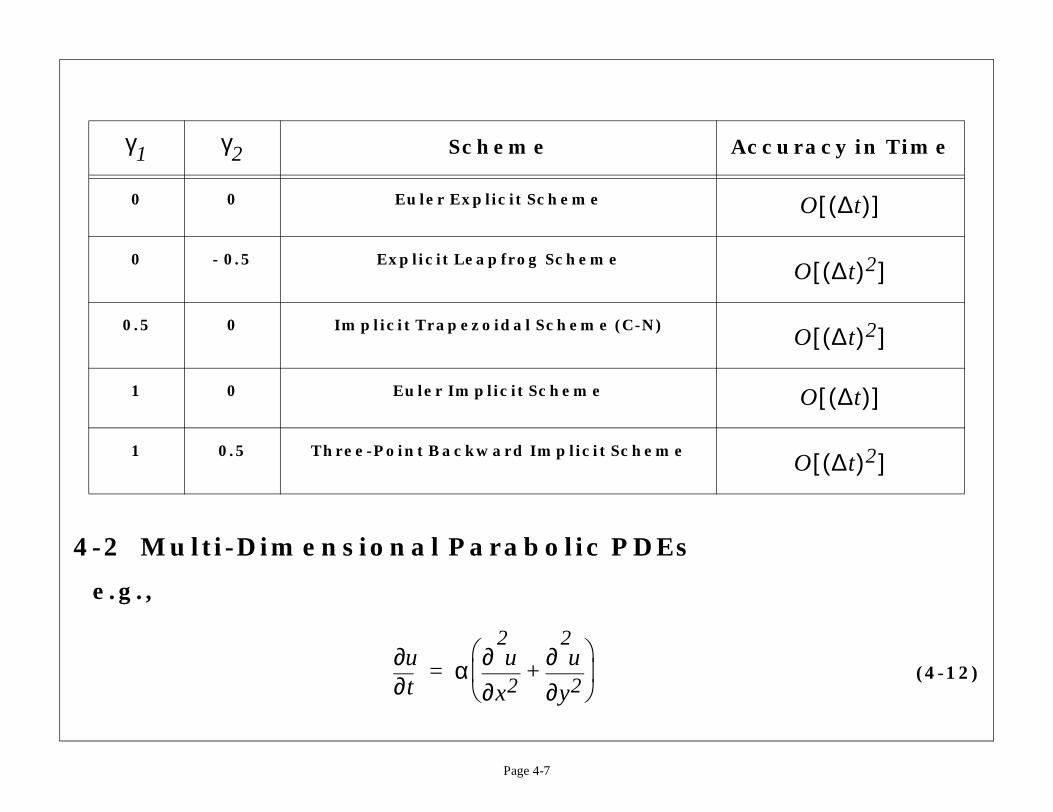
4
(4-12)
Accuracy in Time
O ∆t( )[ ]
O ∆t( )2[ ]
O ∆t( )2[ ]
O ∆t( )[ ]
O ∆t( )2[ ]
Page 4-7
-2 Multi-Dimensional Parabolic PDEs
e.g.,
Scheme
0 0 Euler Explicit Scheme
0 - 0.5 Explicit Leapfrog Scheme
0.5 0 Implicit Trapezoidal Scheme (C-N)
1 0 Euler Implicit Scheme
1 0.5 Three-Point Backward Implicit Scheme
γ1 γ2
t∂∂u α
x2
2
∂∂ u
y2
2
∂∂ u
+
=
(4-13)i j, 1–n
---------------
i
j
n
x
y
α∆ t
∆y( )2--------------
12--- or d
14---≤
Page 4-8
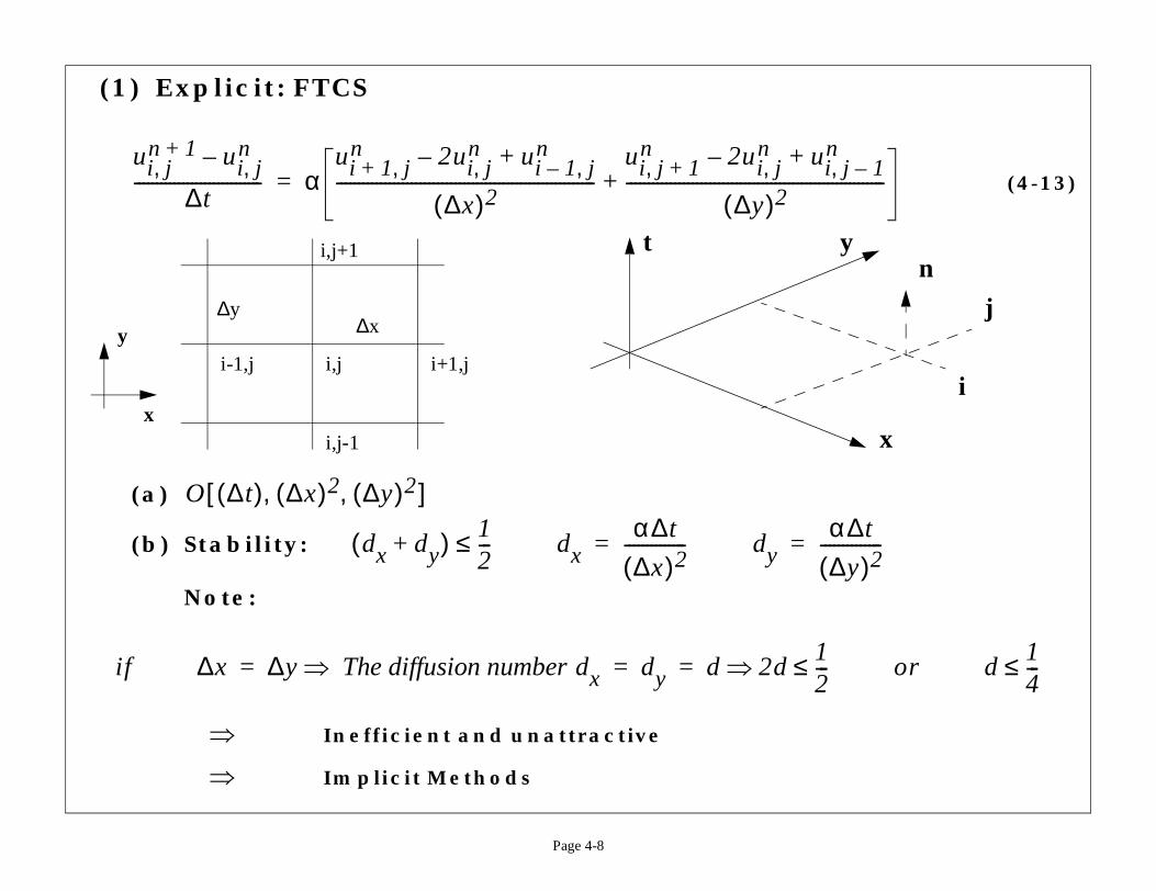
(1) Explicit: FTCS
(a)
(b) Stability:
Note:
Inefficient and unattractive
Implicit Methods
ui j,n 1+ ui j,
n–
∆t----------------------------- α
ui 1 j,+n 2ui j,
n– ui 1 j,–n+
∆x( )2-----------------------------------------------------------
ui j, 1+n 2ui j,
n– u+
∆y( )2--------------------------------------------+=
∆y∆x
i-1,j i,j i+1,j
i,j-1
i,j+1
x
y
t
O ∆t( ) ∆x( )2 ∆y( )2, ,[ ]
dx dy+( ) 12---≤ dx
α∆ t
∆x( )2--------------= dy =
if ∆x ∆y The diffusion number dx⇒ dy d 2d ≤⇒= = =
⇒
⇒
(4-14)
(4-15)
(4-16)
ed Matrix
j1+ ui j, 1–
n 1++
)2------------------------------
i j 1+,n 1+ ui j,
n–=
1+1 fi j,=
.......................
........................
............................ .
.
.
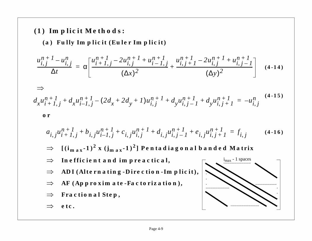
imax - 1 spaces
Page 4-9
(1) Implicit Methods:
(a) Fully Implicit (Euler Implicit)
or
[(imax-1)2 x (jmax-1)2] Pentadiagonal band
Inefficient and impreactical,
ADI (Alternating-Direction-Implicit),
AF (Approximate-Factorization),
Fractional Step,
etc.
ui j,n 1+ ui j,
n–
∆t----------------------------- α
ui 1 j,+n 1+ 2ui j,
n 1+– ui 1 j,–n 1++
∆x( )2-----------------------------------------------------------------
ui j, 1+n 1+ 2ui,
n–
∆y(-----------------------------------+=
⇒
dxui 1 j,+n 1+ dxui 1– j,
n 1+ 2dx 2dy 1+ +( )ui j,n 1+ dyui j 1–,
n 1+ dyu+ +–+
ai j, ui 1 j,+n 1+ bi j, ui 1– j,
n 1+ ci j, ui j,n 1+ di j, ui j 1–,
n 1+ ei j, ui j,n ++ + + +
⇒
⇒
⇒
⇒
⇒
⇒
..........
.
.
.
(4-17)
i j, ui j, 1–+ )n
y)2-----------------------------------
i j, ui j, 1–+ )n 1+
∆y)2-----------------------------------------
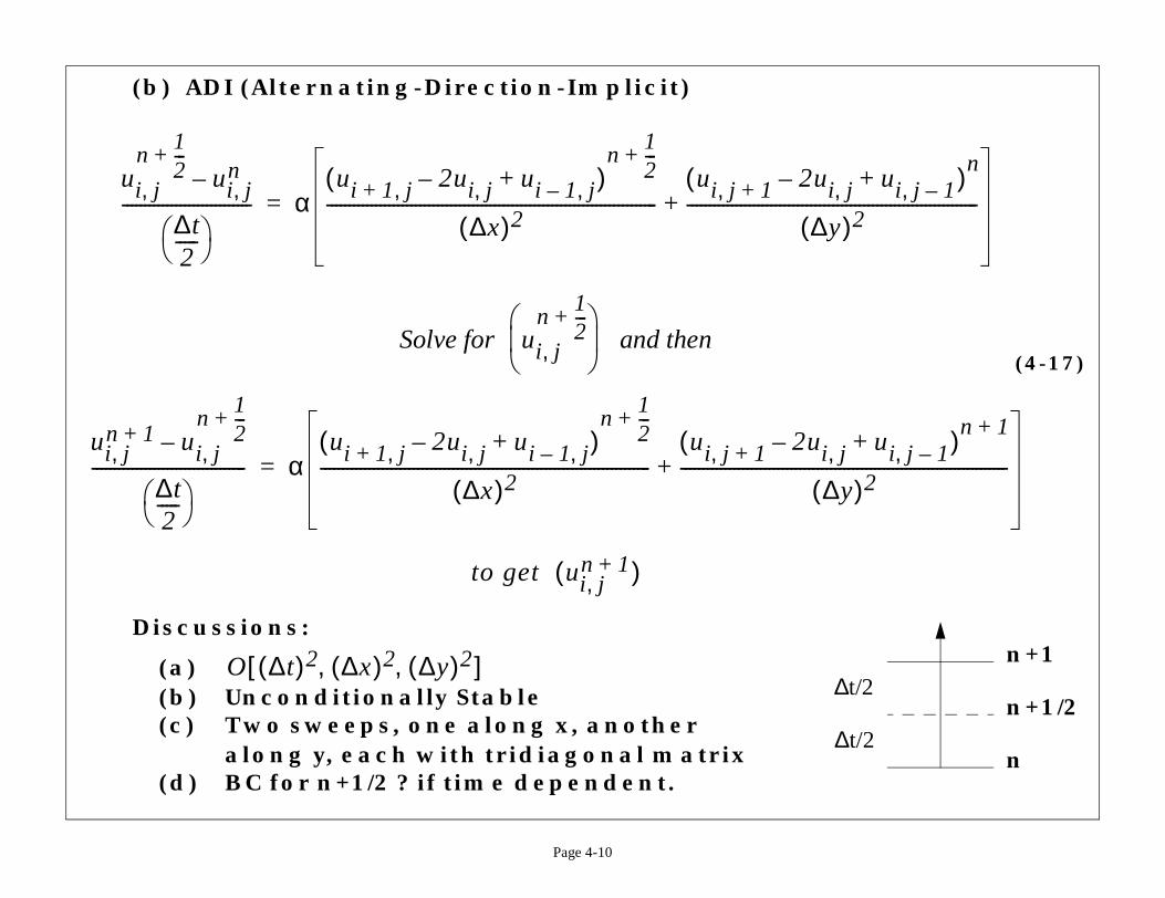
n+1
n+1/2
n
∆t/2
∆t/2
Page 4-10
(b) ADI (Alternating-Direction-Implicit)
Discussions:
(a)(b) Unconditionally Stable(c) Two sweeps, one along x, another
along y, each with tridiagonal matrix(d) BC for n+1/2 ? if time dependent.
ui j,n
12---+
ui j,n–
∆t2-----
----------------------------- αui 1 j,+ 2ui j,– ui 1 j,–+( )
n12---+
∆x( )2---------------------------------------------------------------------------
ui j, 1+ 2u–(
∆(-------------------------------+=
Solve for ui j,n
12---+
and then
ui j,n 1+ ui j,
n12---+
–
∆t2-----
----------------------------------- αui 1 j,+ 2ui j,– ui 1 j,–+( )
n12---+
∆x( )2---------------------------------------------------------------------------
ui j, 1+ 2u–(
(---------------------------------+=
to get ui j,n 1+( )
O ∆t( )2 ∆x( )2 ∆y( )2, ,[ ]
(4-18)
(4-19)
AF⇒
t∂∂u
i j,
n
α∆ t
∆x)2------------
α∆ t
∆y)2------------
j dyδy2ui j,
n+ )
Page 4-11
(c) AF (Approximate-Factorization)
Recall
Define
then for , we have
ADI AF⊂ and LU Decomposition
∆ui j,n
∆t------------- β
t∂∂u
i j,
n 1+1 β–( )
t∂∂u
i j,
n+=
⇒ ui j,n 1+ β ∆t( )
t∂∂u
i j,
n 1+– ui j,
n 1 β–( ) ∆t( )+=
δx2ui j, ui 1+ j, 2ui j,– ui 1– j,+= dx (
--=
δy2ui j, ui j 1+, 2ui j,– ui j 1–,+= dy (
--=
t∂∂u α
x2
2
∂∂ u
y2
2
∂∂ u
+
=
ui j,n 1+ β dxδx
2ui j,n 1+ dyδy
2ui j,n 1++( )– ui j,
n 1 β–( ) dxδx2ui,
n(+=
(4-20)
(4-21)
(4-22)
quence
(4-23)
(4-24)
(4-25)
ui j,*
i j,n 1+
Page 4-12
or
where
By AF, (4-20) becomes
(4-22) is solved according to the following se
Discussions:(a) (4-24) into (4-23), gives
1 β dxδx2 dyδy
2+( )–[ ] ui j,n 1+ RHS( )i j,
n=
RHS( )i j,n 1 1 β–( ) dxδx
2 dyδy2+( )+[ ] ui j,
n=
1 βdxδx2–( ) 1 βdyδy
2–( )ui j,n 1+ RHS( )i j,
n=
1 βdxδx2–( )ui j,
* RHS( )i j,n= Solve for
1 βdyδy2–( )ui j,
n 1+ ui j,*= Solve for u
1 βdxδx2–( ) 1 βdyδy
2–( )ui j,n 1+ RHS( )i j,
n=
(4-26)
(4-27)
(4-28)
(4-29)
(4-29) is
)i j,n
)dyδy2] ui j,
n
r! OK⇒
Page 4-13
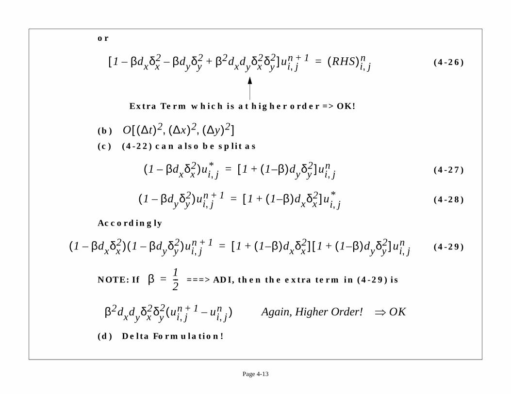
or
(b)
(c) (4-22) can also be split as
Accordingly
NOTE: If ===> ADI, then the extra term in
(d) Delta Formulation!
1 βdxδx2 βdyδy
2 β2dxdyδx2δy
2+––[ ] ui j,n 1+ RHS(=
Extra Term which is at higher order => OK!
O ∆t( )2 ∆x( )2 ∆y( )2, ,[ ]
1 βdxδx2–( )ui j,
* 1 1 β–( )dyδy2+[ ] ui j,
n=
1 βdyδy2–( )ui j,
n 1+ 1 1 β–( )dxδx2+[ ] ui j,
*=
1 βdxδx2–( ) 1 βdyδy
2–( )ui j,n 1+ 1 1 β–( )dxδx
2+[ ] 1 1 β–(+[=
β 12---=
β2dxdyδx2δy
2 ui j,n 1+ ui j,
n–( ) Again, Higher Orde
1
(4-30)
type in x or y
Type in y or x
n
y2
2
∂∂ u
n
12---+
+
Page 4-14
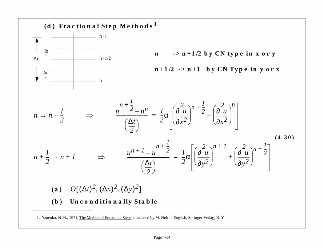
(d) Fractional Step Methods
(a)
(b) Unconditionally Stable
1. Yanenko, N. N., 1971, The Method of Fractional Steps, translated by M. Holt in English, Springer-Verlag, N. Y.
n -> n+1/2 by CN
n+1/2 -> n+1 by CN
n
n+1/2
n+1
∆t2-----
∆t2-----
∆t
n n12---+→ ⇒ u
n12---+
un–
∆t2-----
--------------------------12---α
x2
2
∂∂ u
n
12---+
x2
2
∂∂ u
+=
n12---+ n 1+→ ⇒ un 1+ u
n12---+
–
∆t2-----
----------------------------------12---α
y2
2
∂∂ u
n 1+
=
O ∆t( )2 ∆x( )2 ∆y( )2, ,[ ]
(4-31)
(4-32)
13---∆t
Page 4-15
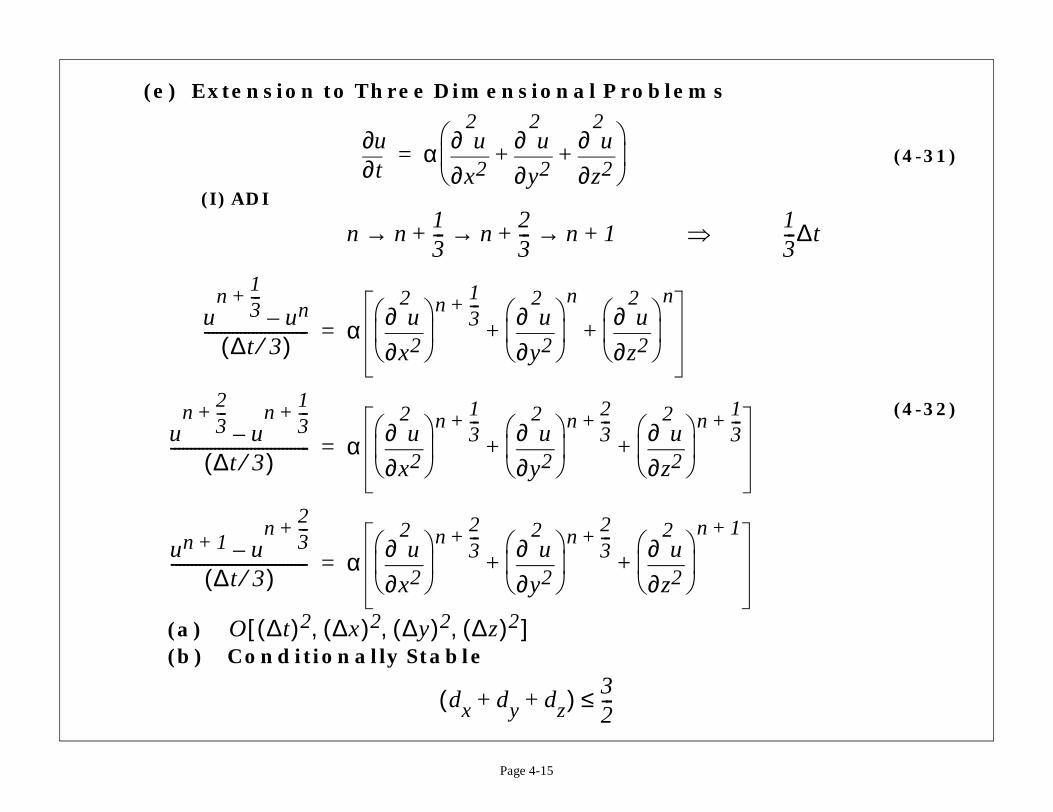
(e) Extension to Three Dimensional Problems
(I) ADI
(a)(b) Conditionally Stable
t∂∂u α
x2
2
∂∂ u
y2
2
∂∂ u
z2
2
∂∂ u
+ +
=
n n13---+ n
23---+ n 1+→ → → ⇒
un
13---+
un–∆t 3⁄( )
-------------------------- αx2
2
∂∂ u
n
13---+
y2
2
∂∂ u
n
z2
2
∂∂ u
n
+ +=
un
23---+
un
13---+
–∆t 3⁄( )
----------------------------------- αx2
2
∂∂ u
n
13---+
y2
2
∂∂ u
n
23---+
z2
2
∂∂ u
n
13---+
+ +=
un 1+ un
23---+
–∆t 3⁄( )
---------------------------------- αx2
2
∂∂ u
n
23---+
y2
2
∂∂ u
n
23---+
z2
2
∂∂ u
n 1+
+ +=
O ∆t( )2 ∆x( )2 ∆y( )2 ∆z( )2, , ,[ ]
dx dy dz+ +( ) 32---≤
(4-33)
z2
2u
n
n
z2
2
∂∂ u
n
+
z2
2
∂∂ u
n 1+
z2
2
∂∂ u
n
+
S)i j k, ,n
RHS)i j k, ,n
Page 4-16
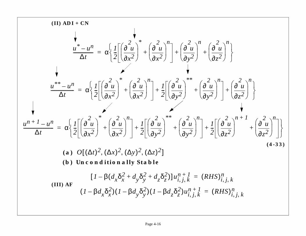
(II) ADI + CN
(a)
(b) Unconditionally Stable
(III) AF
u* un–∆t
----------------- α 12---
x2
2
∂∂ u
*
x2
2
∂∂ u
n
+y2
2
∂∂ u
n
∂∂
+ +
=
u** un–∆t
-------------------- α 12---
x2
2
∂∂ u
*
x2
2
∂∂ u
n
+12---
y2
2
∂∂ u
**
y2
2
∂∂ u
++
=
un 1+ un–∆t
-------------------------- α 12---
x2
2
∂∂ u
*
x2
2
∂∂ u
n
+12---
y2
2
∂∂ u
**
y2
2
∂∂ u
n
+12---+ +
=
O ∆t( )2 ∆x( )2 ∆y( )2 ∆z( )2, , ,[ ]
1 β dxδx2 dyδy
2 dzδz2+ +( )–[ ] ui j k, ,
n 1+ RH(=
1 βdxδx2–( ) 1 βdyδy
2–( ) 1 βdzδz2–( )ui j k, ,
n 1+ (=
(4-34)
(4-35)ui j 1–,----------------- 0=
Page 4-17
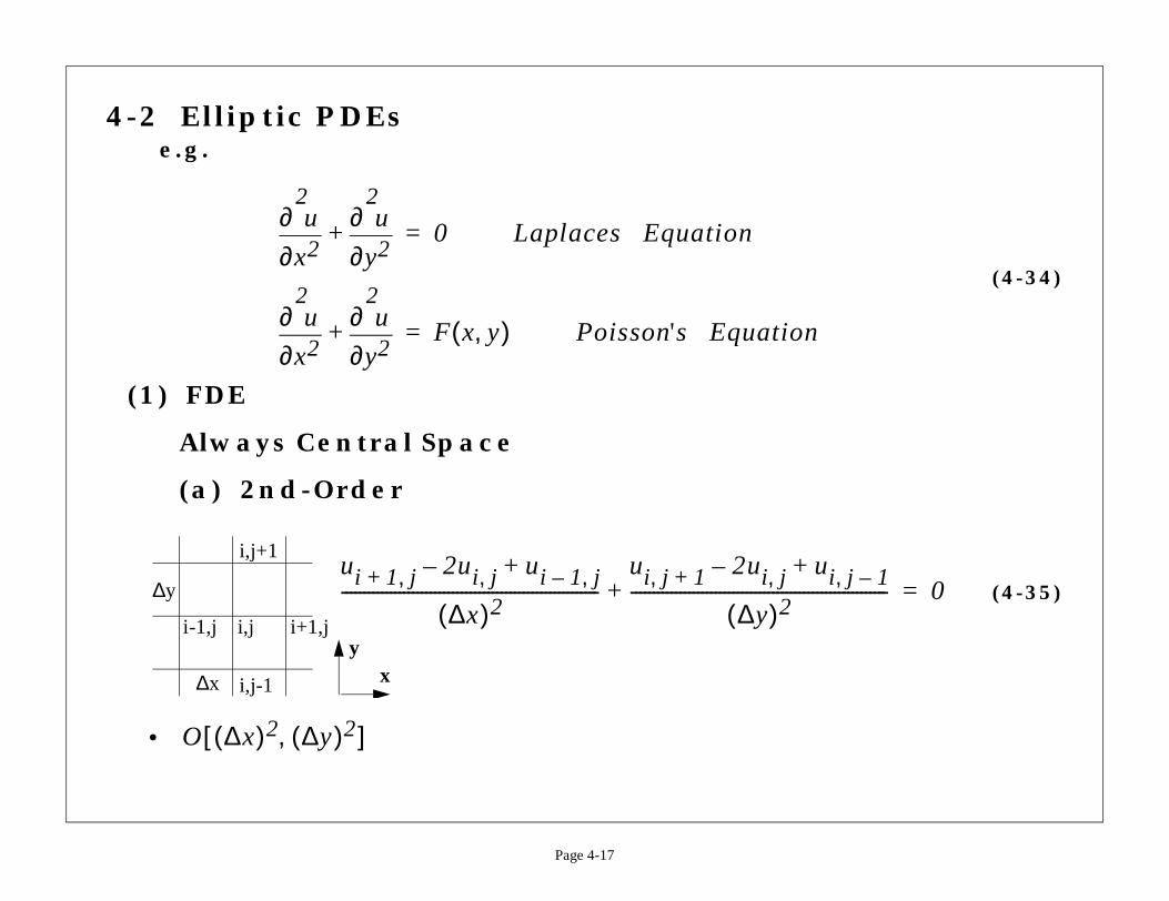
4-2 Elliptic PDEse.g.
(1) FDE
Always Central Space
(a) 2nd-Order
•
x2
2
∂∂ u
y2
2
∂∂ u
+ 0= Laplaces Equation
x2
2
∂∂ u
y2
2
∂∂ u
+ F x y,( )= Poisson's Equation
ui 1 j,+ 2ui j,– ui 1 j,–+
∆x( )2----------------------------------------------------------
ui j 1+, 2ui j,– +
∆y( )2-----------------------------------------+∆y
∆x
i-1,j i,j i+1,j
i,j-1
i,j+1
xy
O ∆x( )2 ∆y( )2,[ ]
(4-36)
j--
i j, 2+--------------- 0=
Page 4-18
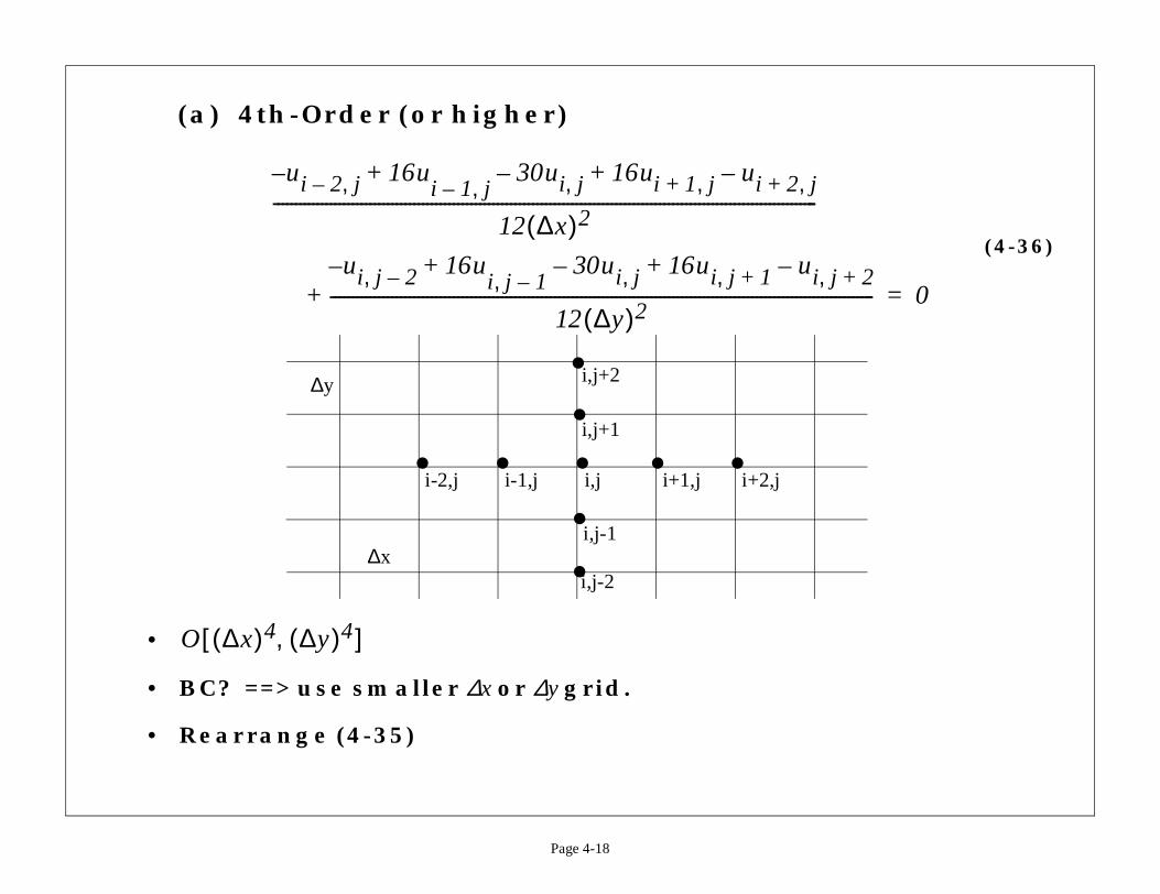
(a) 4th-Order (or higher)
•
• BC? ==> use smaller ∆x or ∆y grid.
• Rearrange (4-35)
ui 2 j,– 16u+–i 1 j,–
30ui j,– 16ui 1 j,+ ui 2,+–+
12 ∆x( )2--------------------------------------------------------------------------------------------------------------------------
ui j, 2– 16u+–i j, 1–
30ui j,– 16ui j, 1+ u–+
12 ∆y( )2-------------------------------------------------------------------------------------------------------------+
i-2,j i-1,j i,j i+1,j i+2,j
i,j+2
i,j+1
i,j-1
i,j-2
∆y
∆x
O ∆x( )4 ∆y( )4,[ ]
(4-37)
or small and dense,
for large, sparse
β ∆x∆y------=
.......
.........
..
.........
.
.
.
Page 4-19
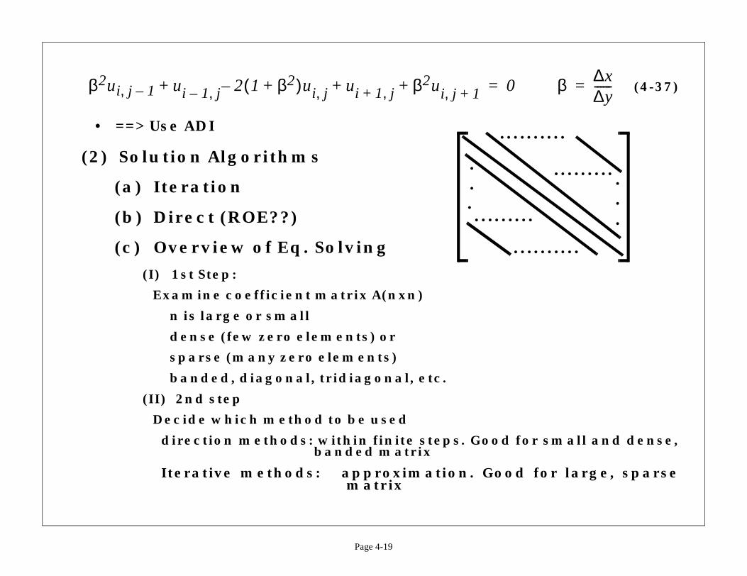
• ==> Use ADI
(2) Solution Algorithms
(a) Iteration
(b) Direct (ROE??)
(c) Overview of Eq. Solving
(I) 1st Step:
Examine coefficient matrix A(nxn)
n is large or small
dense (few zero elements) or
sparse (many zero elements)
banded, diagonal, tridiagonal, etc.
(II) 2nd step
Decide which method to be used
direction methods: within finite steps. Good fbanded matrix
Iterative methods: approximation. Goodmatrix
β2ui j 1–, ui 1– j, 2 1 β2+( )ui j,– ui 1 j,+ β2u+ i j 1+,++ 0=
...
.......
.
.
..
root and f(x) = 0
x( ) ax3 bx2 cx d–+ +=
x) ax h bx( )tan–=
x( ) x2 7–=
*)x– )
----------
f x*( )f ' x*( )---------------–
g Iteration Function≡
x
x1
gy=x
Page 4-20
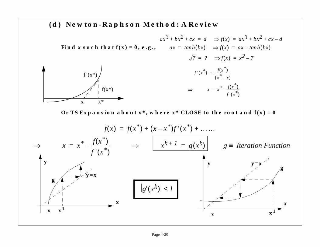
(d) Newton-Raphson Method: A Review
Find x such that f(x) = 0, e.g.,
Or TS Expansion about x*, where x* CLOSE to the
ax3 bx2 cx+ + d f⇒=
ax h bx( )tan f(⇒=
7 ? f⇒=
f(x*)
x*x
f’(x*) f ' x*( ) f x(x*(
---------=
⇒ x x*=
f x( ) f x*( ) x x*–( )f ' x*( ) ……+ +=
⇒ x x* f x*( )f ' x*( )---------------–= ⇒ xk 1+ g xk( )=
y=x
x x1x
y
g
y
x
g' xk( ) 1<
(4-38)
) vector. Iterative
such that
(4-39)
(4-40)
.
(4-41)
, .....
k 1+ Φk≈
aii 0≠
0 i j≥aij i j<
Page 4-21
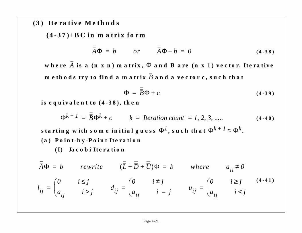
(3) Iterative Methods
(4-37)+BC in matrix form
where is a (n x n) matrix, and B are (n x 1
methods try to find a matrix and a vector c,
is equivalent to (4-38), then
starting with some initial guess , such that
(a) Point-by-Point Iteration
(I) Jacobi Iteration
AΦ b= or AΦ b– 0=
A Φ
B
Φ BΦ c+=
Φk 1+ BΦk c+= k Iteration count = 1, 2, 3=
Φ1 Φ
AΦ b= rewrite L D U+ +( )Φ b= where
lij0 i j≤aij i j>
= dij
0 i j≠aij i j=
= uij
=
(4-42)
(4-43)
U)Φ D1–
b+
i
2k x3
k 12+– )
0 x3k 12+– )
x2k 0 12+ + )
Page 4-22
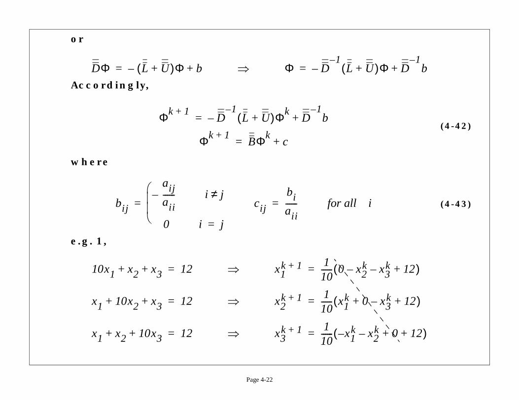
or
Accordingly,
where
e.g. 1,
DΦ L U+( )Φ– b+= ⇒ Φ D1–
L +(–=
Φk 1+D
1–L U+( )Φk
– D1–b+=
Φk 1+BΦk
c+=
bij
aijaii------– i j≠
0 i j=
= cij
biaii------= for all
10x1 x2 x3+ + 12= ⇒ x1k 1+ 1
10------ 0 x–(=
x1 10x2 x3+ + 12= ⇒ x2k 1+ 1
10------ x1
k +(=
x1 x2 10x3+ + 12= ⇒ x3k 1+ 1
10------ x– 1
k –(=
(4-44)
(4-45)
(4-46)
ach (Parabolic) ==>
dy
ui j 1+,
0= β ∆x∆y------=
1 j, β2ui j 1+,k+ ]
Page 4-23
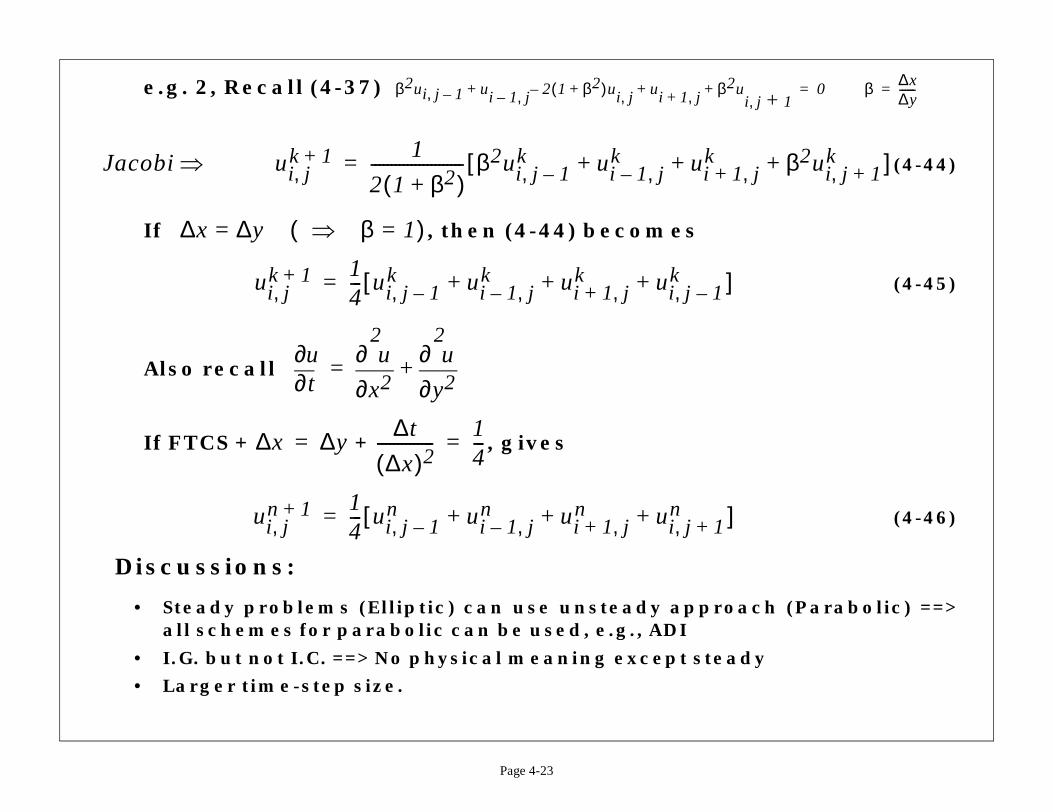
e.g. 2, Recall (4-37)
If , then (4-44) becomes
Also recall
If FTCS + + , gives
Discussions:
• Steady problems (Elliptic) can use unsteady approall schemes for parabolic can be used, e.g., ADI
• I.G. but not I.C. ==> No physical meaning except stea
• Larger time-step size.
β2ui j 1–, ui 1– j, 2 1 β2+( )ui j,– ui 1 j,+ β2+++
Jacobi ⇒ ui j,k 1+ 1
2 1 β2+( )----------------------- β2ui j 1–,
k ui 1– j,k ui +
k+ +[=
∆x ∆y= β⇒ 1=( )
ui j,k 1+ 1
4--- ui j 1–,
k ui 1– j,k ui 1+ j,
k ui j 1–,k++ +[ ]=
t∂∂u
x2
2
∂∂ u
y2
2
∂∂ u
+=
∆x ∆y=∆t
∆x( )2--------------
14---=
ui j,n 1+ 1
4--- ui j 1–,
n ui 1– j,n ui 1+ j,
n ui j 1+,n++ +[ ]=
(4-47)
(4-48)
Φk b+
k 1+ BΦk c+=
k b+
k b+ ]
aijΦjk
j i>∑ bi+
----------------------------------
Page 4-24
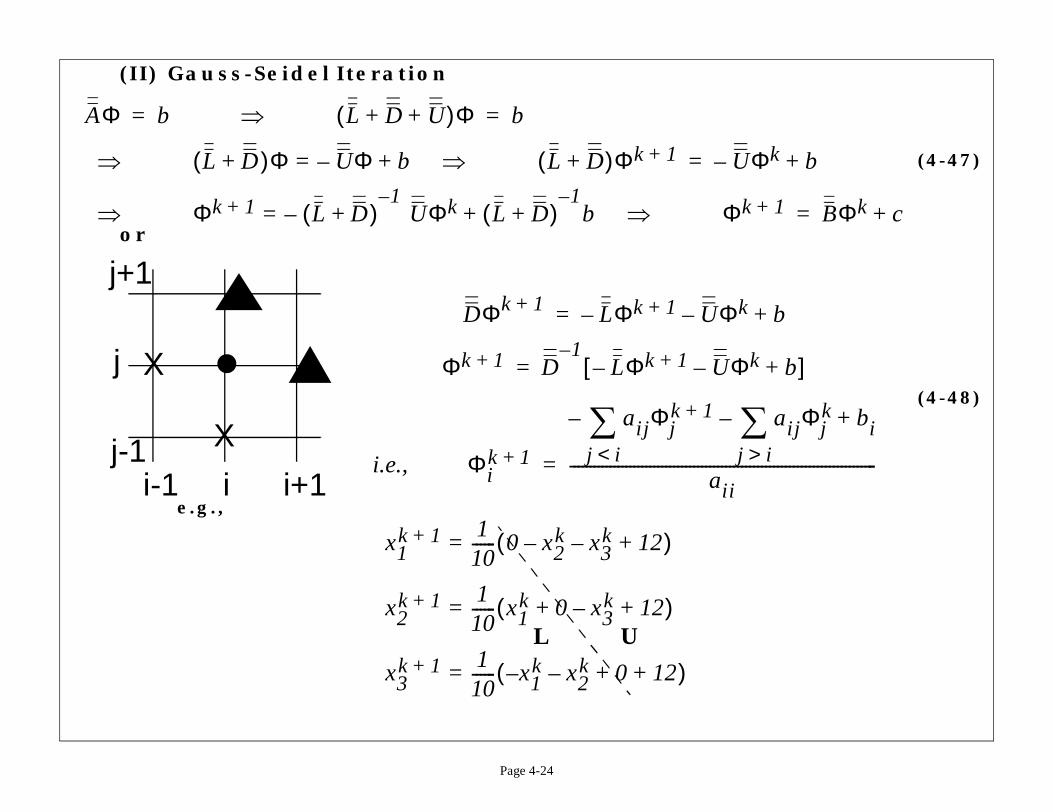
(II) Gauss-Seidel Iteration
or
e.g.,
AΦ b= ⇒ L D U+ +( )Φ b=
⇒ L D+( )Φ UΦ– b+= ⇒ L D+( )Φk 1+ U–=
⇒ Φk 1+ L D+( )1–
UΦk– L D+( )1–
b+= ⇒ Φ
DΦk 1+ LΦk 1+ UΦ––=
Φk 1+ D1–
LΦk 1+ UΦ––[=
i.e., Φik 1+
aijΦjk 1+
j i<∑ ––
aii-------------------------------------------=
X
i-1 i i+1
j+1
j
j-1 X
x1k 1+ 1
10------ 0 x2
k– x3k 12+–( )=
x2k 1+ 1
10------ x1
k 0 x3k 12+–+( )=
x3k 1+ 1
10------ x– 1
k x2k 0 12+ +–( )=
UL
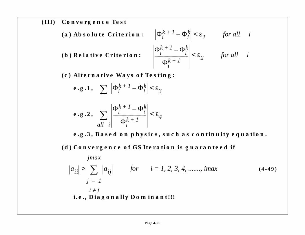
(III) Convergence Test
uity equation.
teed if
(4-49)
for all i
for all i
x
Page 4-25
(a) Absolute Criterion:
(b) Relative Criterion:
(c) Alternative Ways of Testing:
e.g.1,
e.g.2,
e.g.3, Based on physics, such as contin
(d) Convergence of GS Iteration is guaran
i.e., Diagonally Dominant!!!
Φik 1+ Φi
k– ε1<
Φik 1+ Φi
k–
Φik 1+
----------------------------- ε2<
Φik 1+ Φi
k– ε3<∑
Φik 1+ Φi
k–
Φik 1+
----------------------------- ε4<all i∑
aii aij
j 1=
i j≠
jmax
∑> for i = 1, 2, 3, 4, ......., ima
(4-50)
(4-51)
(4-52)
L D U+ +( )Φk– bk+
k
Rk
k ∞→lim 0⇒
L D U+ +( )Φk– bk+=
Page 4-26
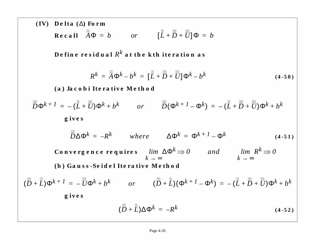
(IV) Delta (∆) Form
Recall
Define residual at the kth iteration as
(a) Jacobi Iterative Method
gives
Convergence requires
(b) Gauss-Seidel Iterative Method
gives
AΦ b= or L D U+ +[ ]Φ b=
Rk
Rk AΦk bk– L D U+ +[ ]Φ k bk–= =
DΦk 1+ L U+( )Φk– bk+= or D Φk 1+ Φk–( ) =
D∆Φk Rk–= where ∆Φk Φk 1+ Φ–=
∆Φk
k ∞→lim 0⇒ and
D L+( )Φk 1+ UΦk– bk+= or D L+( ) Φk 1+ Φk–( )
D L+( )∆Φk Rk–=
(4-53)
a direct method.
have
(4-54)
e, or conditioning
is easily solvable.
(4-55)
(4-56)
Page 4-27
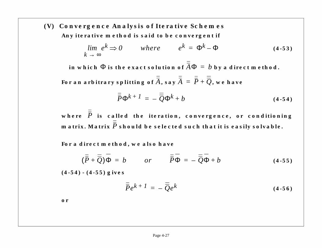
(V) Convergence Analysis of Iterative SchemesAny iterative method is said to be convergent if
in which is the exact solution of by
For an arbitrary splitting of , say , we
where is called the iteration, convergenc
matrix. Matrix should be selected such that it
For a direct method, we also have
(4-54) - (4-55) gives
or
ekk ∞→lim 0⇒ where ek Φk Φ–=
Φ AΦ b=
A A P Q+=
PΦk 1+ QΦk b+–=
P
P
P Q+( )Φ b= or PΦ QΦ b+–=
Pek 1+ Qek–=
(4-57)
trix.
(4-58)
ined by the modulus
(4-59)
…
P1–
Ake1
Page 4-28
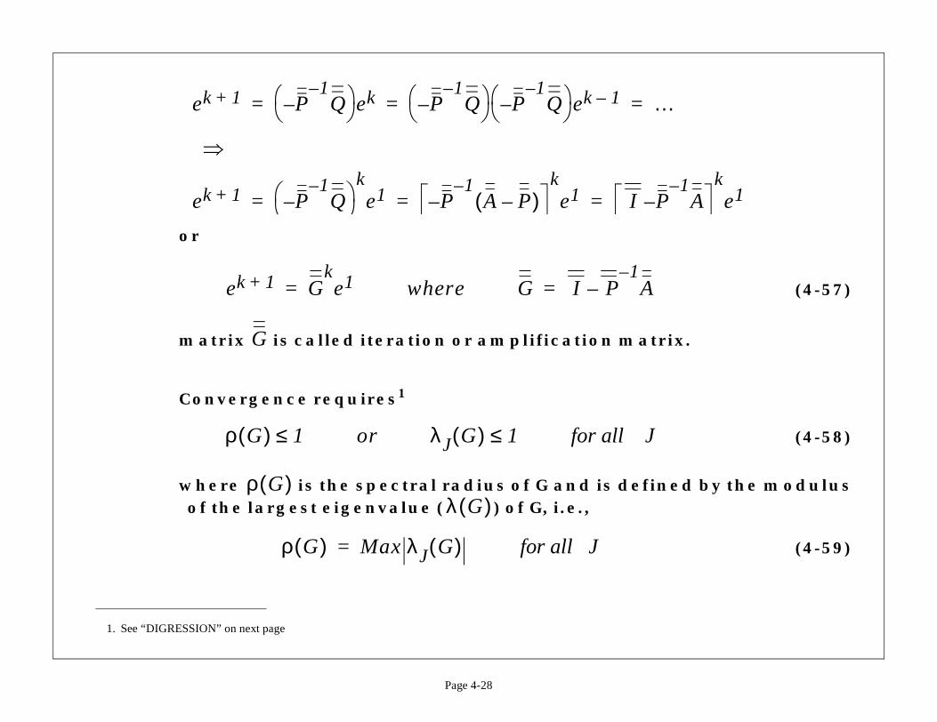
or
matrix is called iteration or amplification ma
Convergence requires1
where is the spectral radius of G and is defof the largest eigenvalue ( ) of G, i.e.,
1. See “DIGRESSION” on next page
ek 1+ P1–
Q– ek P
1–Q–
P1–
Q– ek 1–= = =
⇒
ek 1+ P1–
Q–
ke1 P
1–A P–( )–
ke1 I –= = =
ek 1+ Gke1= where G I P
1–A–=
G
ρ G( ) 1≤ or λJ G( ) 1≤ for all J
ρ G( )λ G( )
ρ G( ) Max λJ G( )= for all J
rs, say , i.e., the
sional vector space
vJ
tion of vJ
k 1+ CJλJkvJ
J 1=
n
∑=
Page 4-29
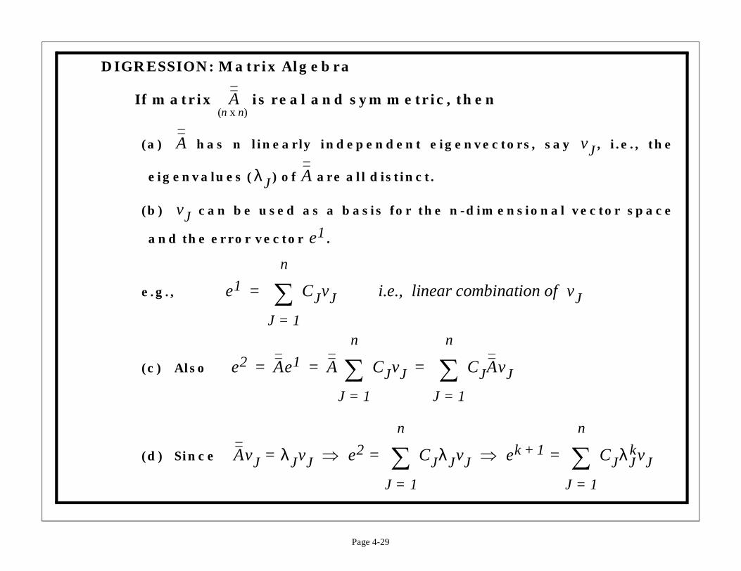
DIGRESSION: Matrix Algebra
If matrix is real and symmetric, then
(a) has n linearly independent eigenvecto
eigenvalues ( ) of are all distinct.
(b) can be used as a basis for the n-dimen
and the error vector .
e.g.,
(c) Also
(d) Since
A(n x n)
A
λJ A
vJ
e1
e1 CJvJ
J 1=
n
∑= i.e., linear combina
e2 Ae1 A CJvJ
J 1=
n
∑ CJAvJ
J 1=
n
∑= = =
AvJ λJvJ= ⇒ e2 CJλJvJ
J 1=
n
∑= ⇒ e
which is easily invertible)
ions can be defined
(4-60)
(4-61)
) I D1–
A–=
D L+ ) 1–A
Page 4-30
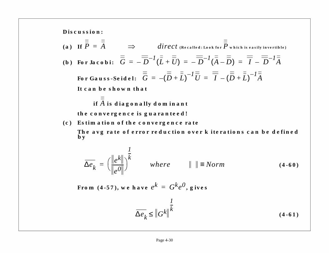
Discussion:
(a) If (Recalled: Look for
(b) For Jacobi:
For Gauss-Seidel:
It can be shown that
if is diagonally dominant
the convergence is guaranteed!
(c) Estimation of the convergence rate
The avg rate of error reduction over k iteratby
From (4-57), we have , gives
P A= ⇒ direct P
G D1–
L U+( )– D1–
A D–(–= =
G D L+( ) 1–U– I (–= =
A
∆ekek
e0----------
1k---
= where Norm≡
ek Gke0=
∆ek Gk
1k---
≤
rix Iterative Analysis.”)
(4-62)
te.rder of magnitude
od
s
mptotically for large k only
hod which dampshigh-frequency
damps poorly therors.
rve.
| | | | | |
i-1 i i+1
x
L
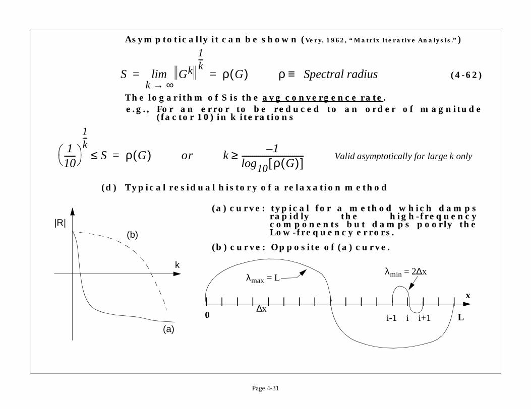
λmin = 2∆x
Page 4-31
Asymptotically it can be shown (Very, 1962, “Mat
The logarithm of S is the avg convergence rae.g., For an error to be reduced to an o
(factor 10) in k iterations
(d) Typical residual history of a relaxation meth
S Gkk ∞→lim
1k---
ρ G( )= = ρ Spectral radiu≡
110------
1k---
S≤ ρ G( )= or k1–
log10 ρ G( )[ ]-------------------------------≥ Valid asy
(a) curve: typical for a metrapidly the components but Low-frequency er
(b) curve: Opposite of (a) cu(b)
(a)
k
|R|
| | | | | | | | | | |
0
λmax = L
∆x
e-Over-Relaxation)
inated problem.
e for linear cases for nonlinear
(4-63)
(4-64)
Φk
n
n
Page 4-32
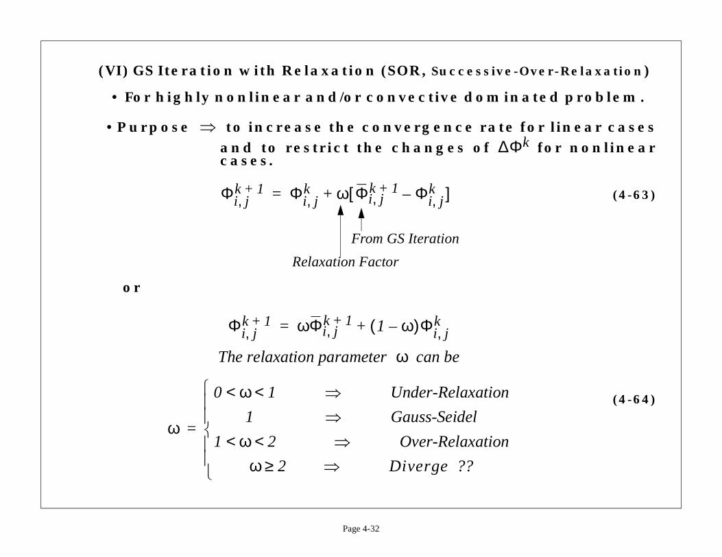
(VI) GS Iteration with Relaxation (SOR, Successiv
• For highly nonlinear and/or convective dom
• Purpose to increase the convergence ratand to restrict the changes of cases.
or
⇒∆
Φi j,k 1+ Φi j,
k ω Φi j,k 1+ Φi j,
k–[ ]+=
From GS Iteration
Relaxation Factor
Φi j,k 1+ ωΦi j,
k 1+ 1 ω–( )Φi j,k+=
The relaxation parameter ω can be
ω
0 ω 1< < ⇒ Under-Relaxatio
1 ⇒ Gauss-Seidel
1 ω 2< < ⇒ Over-Relaxatio
ω 2≥ ⇒ Diverge ??
=
product of its eigen-
)D ωU– ]
er Matrix
1U
0 N = matrix size
R ω( ) 1 ω–( )N=
2<
Page 4-33
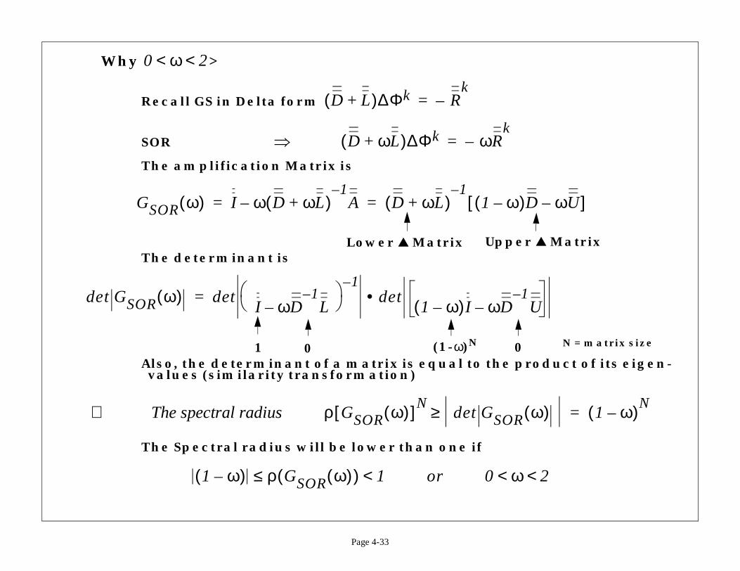
Why >
Recall GS in Delta form
SOR
The amplification Matrix is
The determinant is
Also, the determinant of a matrix is equal to the values (similarity transformation)
The Spectral radius will be lower than one if
0 ω 2< <
D L+( )∆Φk Rk
–=
⇒ D ωL+( )∆Φk ωRk
–=
GSOR ω( ) I ω D ωL+( )1–
A– D ωL+( )1–
1 ω–([= =
Lower Matrix Upp
det GSOR ω( ) detI ωD
1–L–
1–det
1 ω–( )I ωD–
–•=
1 0 (1-ω)N
∴ The spectral radius ρ GSOR ω( )[ ]N det GSO≥
1 ω–( ) ρ GSOR ω( )( ) 1<≤ or 0 ω<
(4-65)
(4-66)
ary information
1 sp+
1 sp+
verticalt, ilast
x x x xE
i
Page 4-34
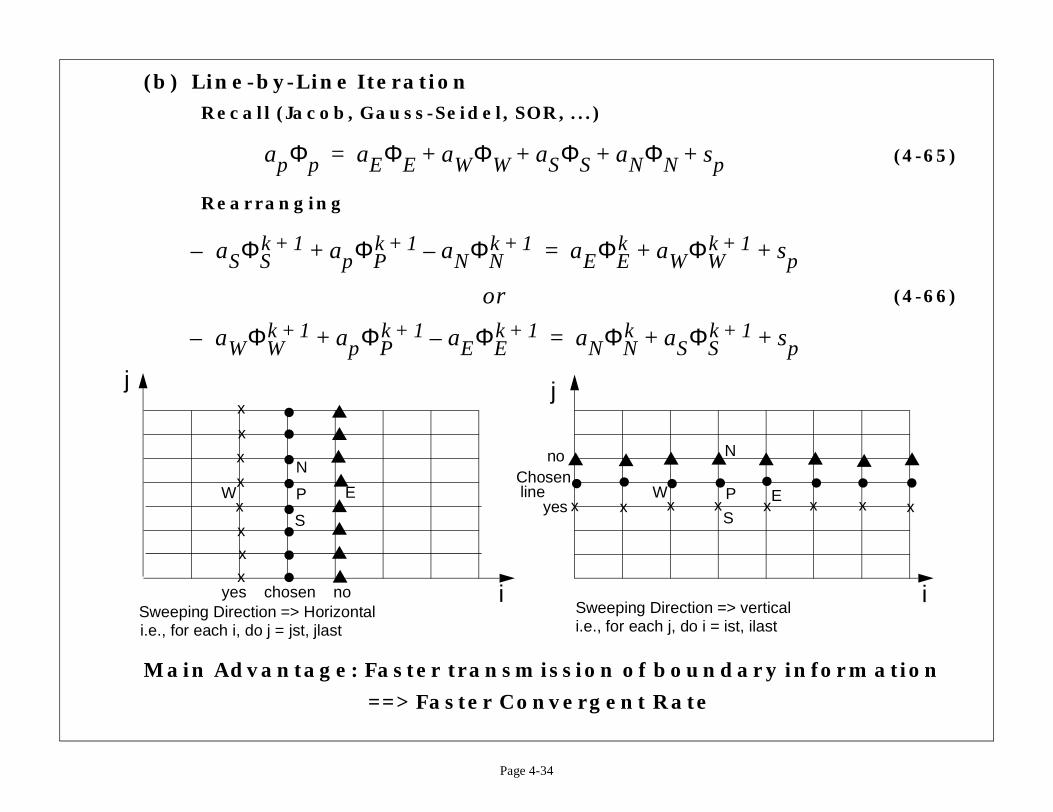
(b) Line-by-Line IterationRecall (Jacob, Gauss-Seidel, SOR, ...)
Rearranging
Main Advantage: Faster transmission of bound
==> Faster Convergent Rate
apΦp aEΦE aWΦW aSΦS aNΦN sp+ + + +=
aSΦSk 1+– apΦP
k 1+ aNΦNk 1+–+ aEΦE
k aWΦWk ++=
or
aWΦWk 1+– apΦP
k 1+ aEΦEk 1+–+ aNΦN
k aSΦSk ++=
W P E
S
N
yes chosen noSweeping Direction => Horizontali.e., for each i, do j = jst, jlast
x
x
x
x
x
xxx
i
j
noChosenline
yes
Sweeping Direction =>i.e., for each j, do i = is
x x x xW P
S
N
j
the boundaryain.
+ Relaxation
Page 4-35
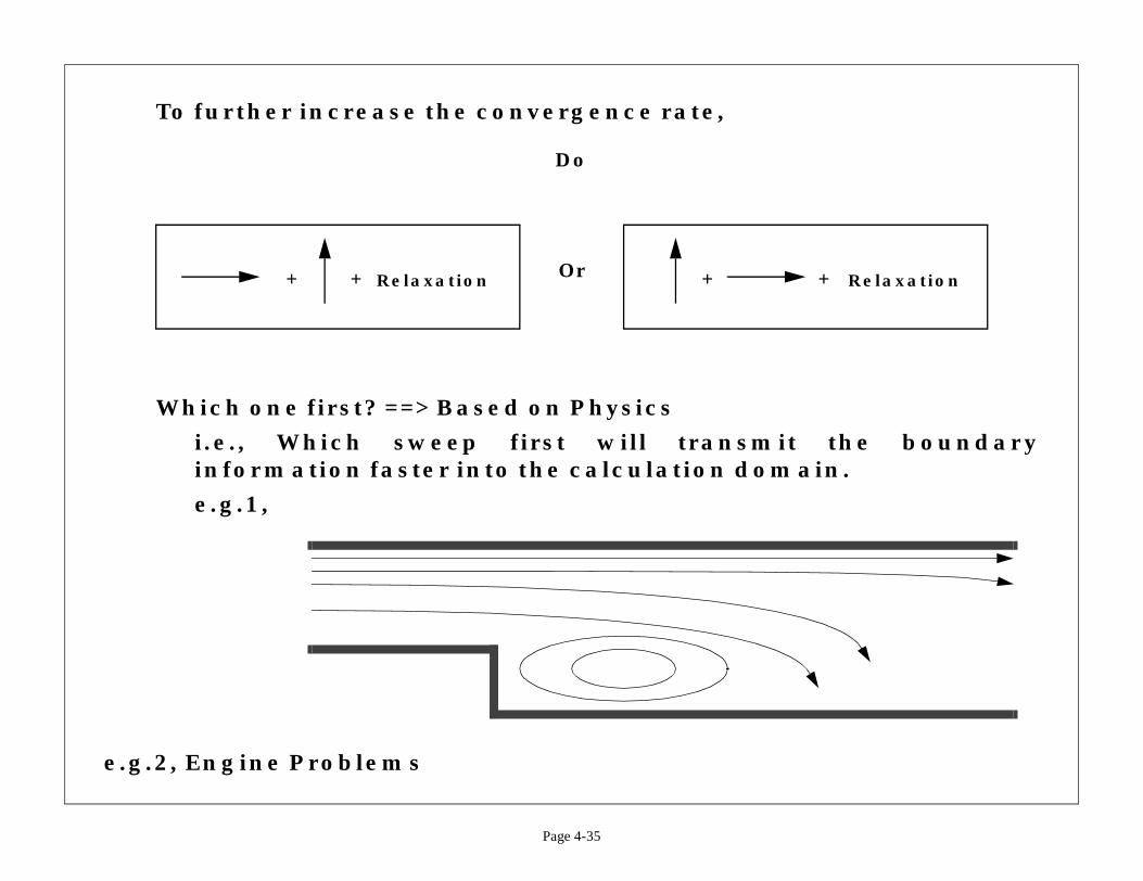
To further increase the convergence rate,
Do
Which one first? ==> Based on Physics
i.e., Which sweep first will transmitinformation faster into the calculation dom
e.g.1,
e.g.2, Engine Problems
Or+ + Relaxation +
(4-67)
0=
t const=
t∂∂u
ax∂∂u
+
stant on
dt⁄ a=
x
u
at
Page 4-36
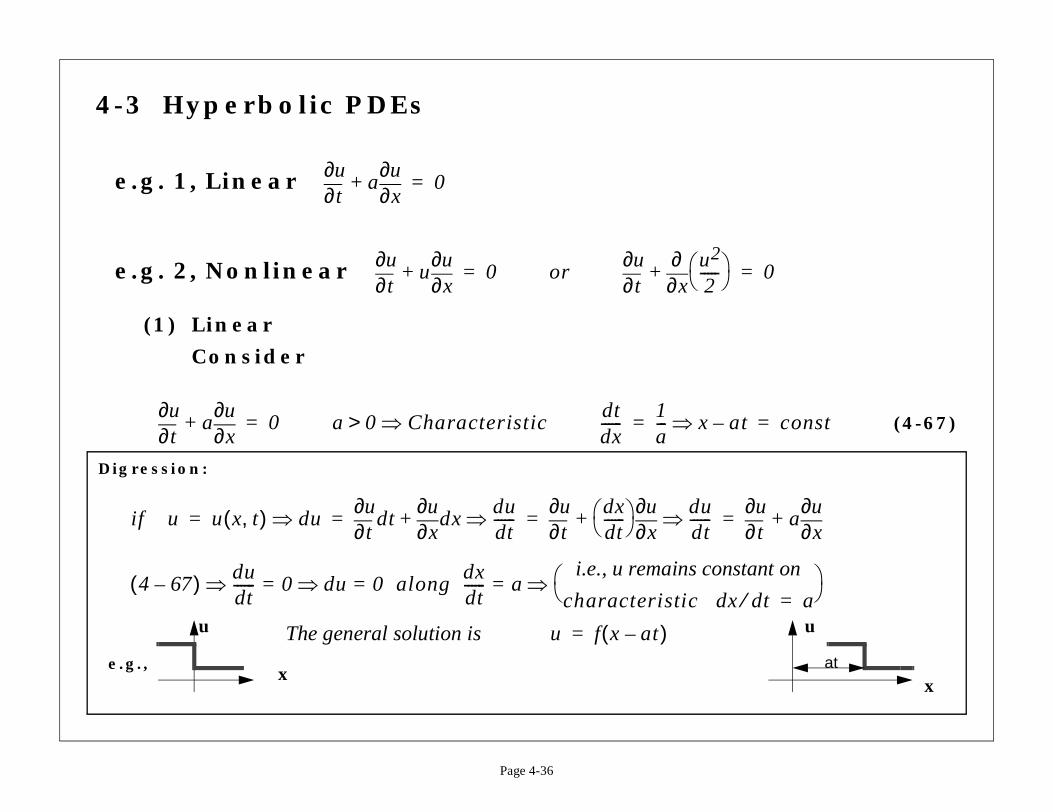
4-3 Hyperbolic PDEs
e.g. 1, Linear
e.g. 2, Nonlinear
(1) Linear
Consider
t∂∂u
ax∂∂u
+ 0=
t∂∂u
ux∂∂u
+ 0= ort∂∂u
x∂∂ u2
2----- +
t∂∂u
ax∂∂u
+ 0= a 0 Characteristic⇒> dtdx------
1a--- x a–⇒=
Digression:
if u u x t,( ) du⇒t∂∂u
dtx∂∂u
dxdudt------⇒+
t∂∂u dx
dt------
x∂∂u
+dudt------⇒= = = =
4 67–( ) dudt------⇒ 0 du⇒ 0= = along
dxdt------ a
i.e., u remains con
characteristic dx⇒=
The general solution is u f x at–( )=e.g.,
x
u
(4-68)
(4-69)
(4-70)
(4-71)
, i.e.,
∆x)].
∆x( )2].
∆x)]
a∆t∆x---------
1≤
a=
Page 4-37
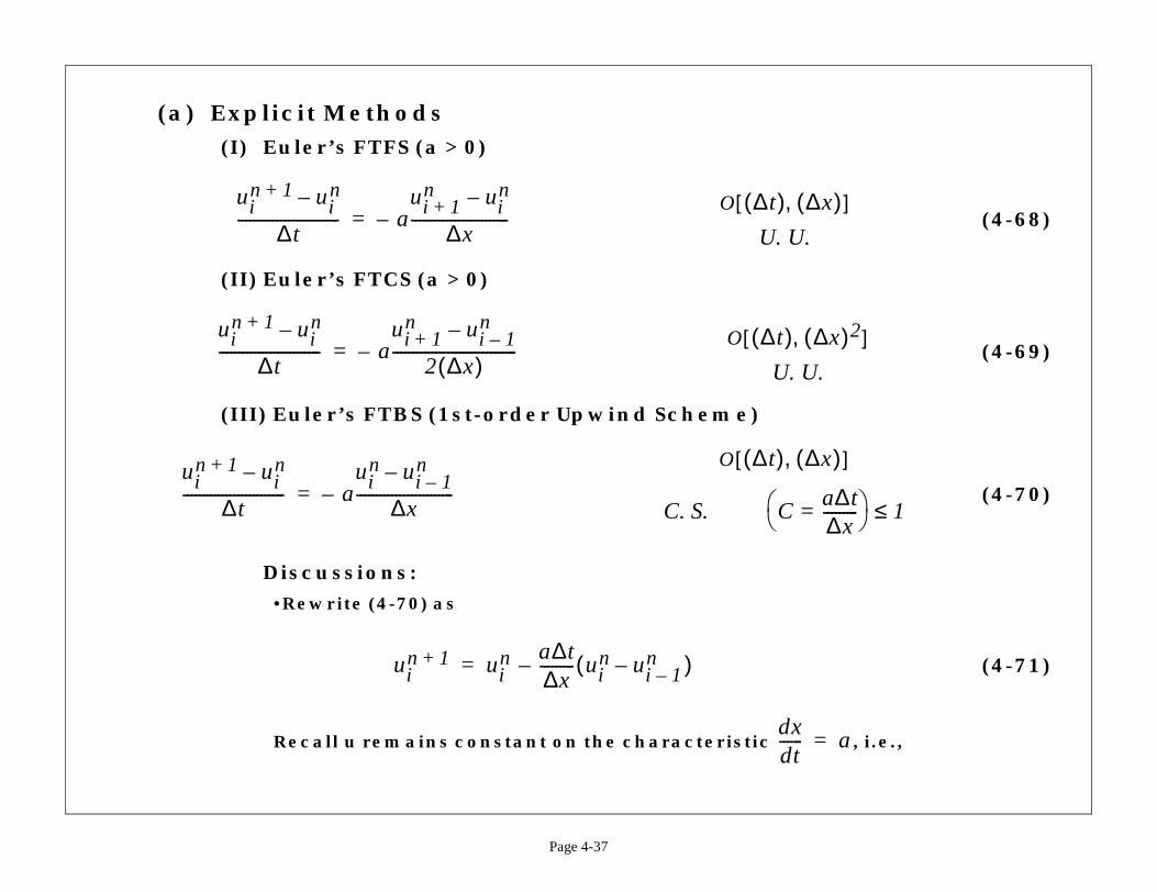
(a) Explicit Methods(I) Euler’s FTFS (a > 0)
(II) Euler’s FTCS (a > 0)
(III) Euler’s FTBS (1st-order Upwind Scheme)
Discussions:
•Rewrite (4-70) as
Recall u remains constant on the characteristic
uin 1+ ui
n–
∆t-------------------------- a
ui 1+n ui
n–
∆x-------------------------–=
O ∆t( ) (,[
U. U
uin 1+ ui
n–
∆t-------------------------- a
ui 1+n ui 1–
n–
2 ∆x( )--------------------------------–=
O ∆t( ),[
U. U
uin 1+ ui
n–
∆t-------------------------- a
uin ui 1–
n–
∆x-------------------------–=
O ∆t( ) (,[
C. S. C =
uin 1+ ui
n a∆t∆x--------- ui
n ui 1–n–( )–=
dxdt------
ation of du/dt = 0 alongolation between i and i-
x
i-1 i
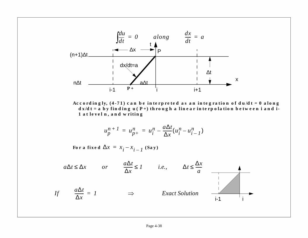
Page 4-38
Accordingly, (4-71) can be interpreted as an integrdx/dt = a by finding u( P+) through a linear interp1 at level n, and writing
For a fixed (Say)
tddu∫ 0= along
dxdt------ a=
dx/dt=a
i-1 i i+1a∆t
∆t
(n+1)∆t
n∆t
tP
P+
∆x
upn 1+ up+
n uin a∆t
∆x--------- ui
n ui 1–n–( )–= =
∆x xi xi 1––=
a∆t ∆x≤ ora∆t∆x--------- 1≤ i.e., ∆t
∆xa
------≤
Ifa∆t∆x--------- 1= ⇒ Exact Solution
(4-72)
, the generale can be written as
(4-73)
nd a
1-----
Page 4-39
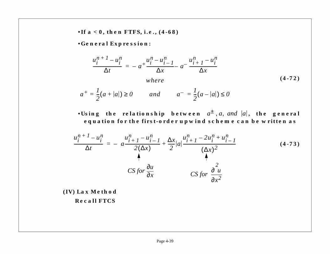
•If a < 0, then FTFS, i.e., (4-68)
•General Expression:
•Using the relationship between equation for the first-order upwind schem
(IV) Lax Method
Recall FTCS
uin 1+ ui
n–
∆t-------------------------- a+
uin ui 1–
n–
∆x------------------------- a–
ui 1+n ui
n–
∆x-------------------------––=
where
a+ 12--- a a+( )= 0≥ and a– 1
2--- a a–( )= 0≤
a± a a, ,
uin 1+ ui
n–
∆t-------------------------- a
ui 1+n ui 1–
n–
2 ∆x( )--------------------------------–
∆x2
------ aui 1+
n 2uin ui –
n+–
∆x( )2------------------------------------------+=
CS forx∂∂u
CS forx2
2
∂∂ u
(4-74)
arting; 2nd-order in
(4-75)
(4-76)
. S. if C 1≤
Page 4-40
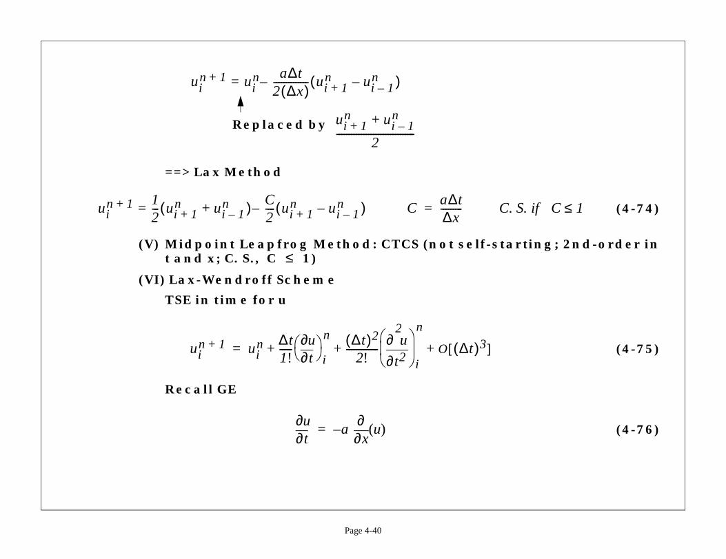
==> Lax Method
(V) Midpoint Leapfrog Method: CTCS (not self-stt and x; C. S., C 1)
(VI) Lax-Wendroff Scheme
TSE in time for u
Recall GE
uin 1+ ui
n a∆t2 ∆x( )-------------- ui 1+
n ui 1–n–( )–=
Replaced by ui 1+n ui 1–
n+
2--------------------------------
uin 1+ 1
2--- ui 1+
n ui 1–n+( ) C
2---- ui 1+
n ui 1–n–( )–= C
a∆t∆x---------= C
≤
uin 1+ ui
n ∆t1!-----
t∂∂u
i
n ∆t( )22!
-------------t2
2
∂∂ u
i
n
O ∆t( )3[ ]+ + +=
t∂∂u
ax∂∂
u( )–=

(4-77)
(4-78)
(4-79)
a2
x2
2
∂∂ u
3]
ui 1–n
-------------
2uin ui 1–
n+
∆x)2---------------------------
Page 4-41
(4-76)+(4-77) into (4-75), gives
Then CS ==>
Discussions:
•
•C. S.,
•Recall 1st-order upwind scheme (4-73)
⇒t2
2
∂∂ u
at∂∂
x∂∂u – a
x∂∂
t∂∂u – a
x∂∂
ax∂∂u
– –= = = =
uin 1+ ui
n ∆t( ) ax∂∂u
–
i
n ∆t( )22
------------- a2
x2
2
∂∂ u
i
n
O ∆t( )[+ + +=
uin 1+ ui
n a ∆t( )–ui 1+
n ui 1–n–
2∆x-------------------------------- a2 ∆t( )2
2-------------------
ui 1+n 2ui
n +–
∆x( )2----------------------------------
+=
O ∆t( )2 ∆x( )2,[ ]
C 1≤
uin 1+ ui
n a ∆t( )ui 1+
n ui 1–n–
2 ∆x( )--------------------------------
–a ∆x( ) ∆t( )
2----------------------------
ui 1+n –
(--------------------
+=
(4-80)
e 1st-order upwind
(4-81)
(4-82)
Page 4-42
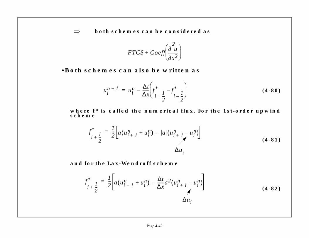
both schemes can be considered as
•Both schemes can also be written as
where f* is called the numerical flux. For thscheme
and for the Lax-Wendroff scheme
⇒
FTCS Coeffx2
2
∂∂ u
+
uin 1+ ui
n ∆t∆x------ f
i12---+
* fi
12---–
*–
–=
fi
12---+
* 12--- a ui 1+
n uin+( ) a– ui 1+
n uin–( )=
∆ui
fi
12---+
* 12--- a ui 1+
n uin+( ) ∆t
∆x------a2– ui 1+
n uin–( )=
∆ui
(4-83)
(4-84)
ms)
∆t( ) ∆x( )2,[ ]
U. S.
Tridiagonal
Physics
∆t)2 ∆x( )2, ]
U. S.
idiagonal
Page 4-43
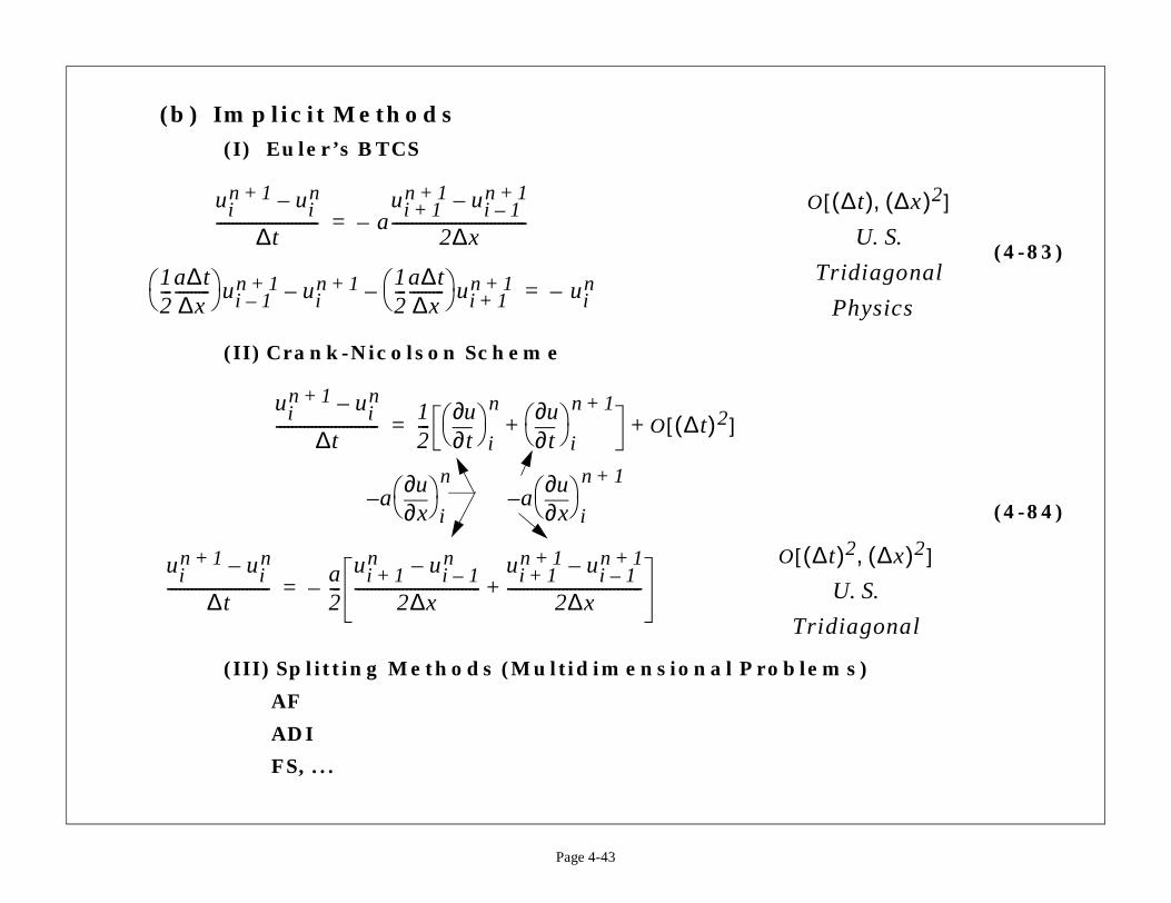
(b) Implicit Methods(I) Euler’s BTCS
(II) Crank-Nicolson Scheme
(III) Splitting Methods (Multidimensional Proble
AF
ADI
FS, ...
uin 1+ ui
n–
∆t-------------------------- a
ui 1+n 1+ ui 1–
n 1+–
2∆x----------------------------------–=
12---
a∆t∆x---------
ui 1–n 1+ ui
n 1+–12---
a∆t∆x---------
ui 1+n 1+– ui
n–=
O
uin 1+ ui
n–
∆t--------------------------
12---
t∂∂u
i
n
t∂∂u
i
n 1++ O ∆t( )2[ ]+=
ax∂∂u –
i
na
x∂∂u –
i
n 1+
uin 1+ ui
n–
∆t--------------------------
a2---
ui 1+n ui 1–
n–
2∆x--------------------------------
ui 1+n 1+ ui 1–
n 1+–
2∆x----------------------------------+–=
O ([
Tr

ethods)
2 Versions)
d as predictor andtor)
(4-85)
(4-86)
Page 4-44
(c) Multi-Step Methods (Predictor-Corrector M
Better for nonlinear equations.
(I) Richtmyer/Lax-Wendroff Multi-Step Method (
(i) Richtmyer Formulation (use Lax MethoBTCS as correc
Predictor (Lax Method at )
Corrector (BTCS)
O ∆t( )2 ∆x( )2,[ ]
ui
n12---+
ui
n12---+ 1
2--- ui 1+
n ui 1–n+( )–
∆t 2⁄( )------------------------------------------------------------- a
ui 1+n ui 1–
n–
2∆x--------------------------------
–=
uin 1+ ui
n–
∆t-------------------------- a
ui 1+
n12---+
ui 1–
n12---+
–
2∆x-----------------------------------
–=
C. S.a∆t∆x--------- 2≤
d as predictor andtor)
(4-87)
(4-88)
)
1 uin–
∆x---------------
Page 4-45
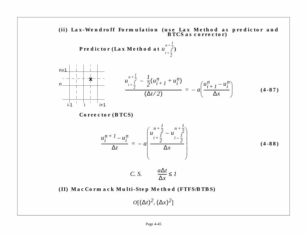
(ii) Lax-Wendroff Formulation (use Lax MethoBTCS as correc
Predictor (Lax Method at )
Corrector (BTCS)
(II) MacCormack Multi-Step Method (FTFS/BTBS
ui
12---+
n12---+
ui
12---+
n12---+ 1
2--- ui 1+
n uin+( )–
∆t 2⁄( )------------------------------------------------------- a
ui +n
----------
–=
i-1 i i+1
n
n+1
XXXX
uin 1+ ui
n–
∆t-------------------------- a
ui
12---+
n12---+
ui
12---–
n12---+
–
∆x---------------------------------
–=
C. S.a∆t∆x--------- 1≤
O ∆t( )2 ∆x( )2,[ ]

(4-89)
(4-90)
1 uin– )
in ui
*+ )
Page 4-46
Predictor: FTFS
Corrector: BTBS
Discussions:
•C. S.
•Can also be
ui* ui
n–
∆t------------------ a
ui 1+n ui
n–
∆x--------------------------
–= i.e., ui* ui
n a∆t∆x--------- ui +
n(–=
uin 1+ ui
**–
∆t 2⁄( )----------------------------- a
ui* ui 1–
*–
∆x--------------------------
–= where ui** 1
2--- u(=
⇒ uin 1+ 1
2--- ui
n ui*+( ) a∆t
∆x--------- ui
* ui 1–*–( )–=
a∆t∆x--------- 1≤
FTBSBTFSFTFSBTBS::
n -> n+1
n+1 -> n+2
(4-91)
(4-92)
uin ui 1–
n– )
Page 4-47
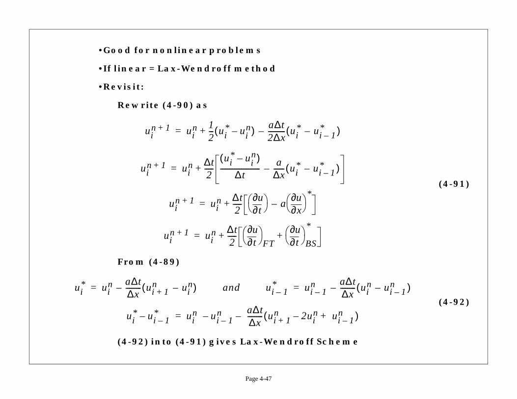
•Good for nonlinear problems
•If linear = Lax-Wendroff method
•Revisit:
Rewrite (4-90) as
From (4-89)
(4-92) into (4-91) gives Lax-Wendroff Scheme
uin 1+ ui
n 12--- ui
* u– in( ) a∆t
2∆x---------- ui
* ui 1–*–( )–+=
uin 1+ ui
n ∆t2-----
ui* u– i
n( )
∆t-----------------------
a∆x------ ui
* ui 1–*–( )–+=
uin 1+ ui
n ∆t2-----
t∂∂u a
x∂∂u
*–+=
uin 1+ ui
n ∆t2-----
t∂∂u
FT t∂∂u
BS
*++=
ui* ui
n a∆t∆x--------- ui 1+
n uin–( )–= and ui 1–
* ui 1–n a∆t
∆x---------(–=
ui* ui 1–
*– uin ui 1–
n a∆t∆x--------- ui 1+
n 2uin– ui 1–
n+( )––=
)
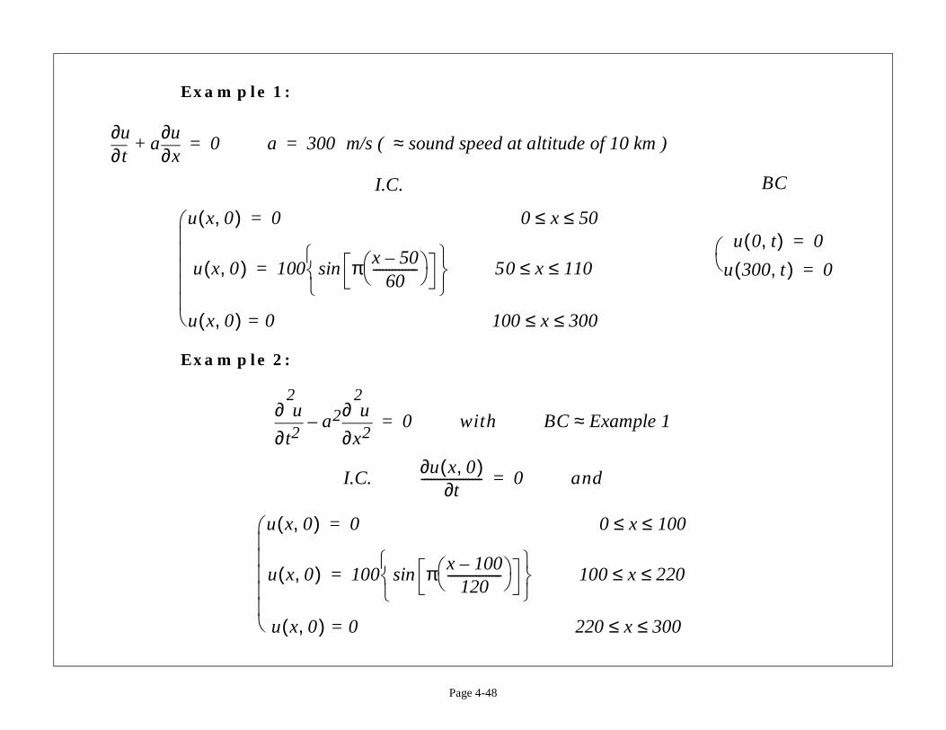
BC
u 0 t,( ) 0=
u 300 t,( ) 0=
1
100
220
00
Page 4-48
Example 1:
Example 2:
t∂∂u
ax∂∂u
+ 0= a 300 m/s ( sound speed at altitude of 10 km≈=
I.C.
u x 0,( ) 0= 0 x 50≤ ≤
u x 0,( ) 100 π x 50–60
-------------- sin
= 50 x 110≤ ≤
u x 0,( ) 0= 100 x 300≤ ≤
t2
2
∂∂ u
a2
x2
2
∂∂ u
– 0= with BC Example≈
I.C.u x 0,( )∂
t∂------------------- 0= and
u x 0,( ) 0= 0 x≤ ≤
u x 0,( ) 100 π x 100–120
----------------- sin
= 100 x≤ ≤
u x 0,( ) 0= 220 x 3≤ ≤

e Scheme1)
ion error
me
t t = n∆t
mes are developed; and (2) the
f E between n & n+1
Page 4-49
(d) Explicit Schemes Revisited
Recall 1st-order upwind scheme
•No oscillations (GOOD!) => monotone variation (Monoton
•Smear out the flow variables (BAD!) => diffusive, dissipat
•Can be considered as a Godunov-Type Scheme
(I) Basic Godunov Scheme•There are three steps involved in the basic Godunov Sche
(1) Define a piecewise constant approximation of u a
(2) Obtain local exact solution at the cell interfaces
(3) Avg the state variables after a time interval ∆t
1. A monotonic scheme is defined by: (1) as the solution proceeds in time, no new local extrelocal minimum is non-decreasing whereas the local maximum is non-increasing.
t∂∂u
x∂∂E
+ 0= a x b≤ ≤ u u x t,( )=
tdd
u x t,( ) xda
b
∫ E b t,( ) E a t,( )–[ ]–=
un 1+ x( ) xdb
∫ un x( ) xdb
∫– ∆t E b( ) E a( )–[ ]–= E time avg o≡
) ) )
u x t,( ) xdi 1 2⁄–( )
i 1 2⁄+( )
∫
a∆t)uin
xd
x x xi-1 i i+1
x
t = (n+1)∆t
Step 3
Page 4-50
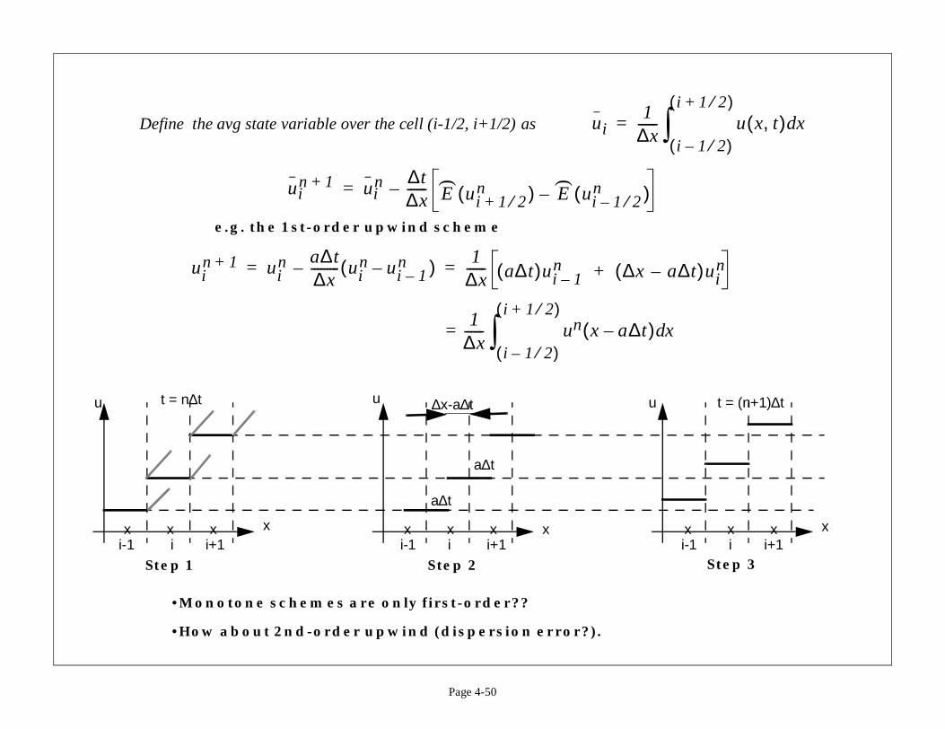
e.g. the 1st-order upwind scheme
•Monotone schemes are only first-order??
•How about 2nd-order upwind (dispersion error?).
Define the avg state variable over the cell (i-1/2, i+1/2) as ui1∆x------=
uin 1+ ui
n ∆t∆x------ E ui 1 2⁄+
n( ) E ui 1 2⁄–n( )––= ) )
uin 1+ ui
n a∆t∆x--------- ui
n ui 1–n–( )–
1∆x------ a∆t( )ui 1–
n ∆x –(+= =
=1∆x------ un x a∆t–( )
i 1 2⁄–( )
i 1 2⁄+( )
∫
x x x x x xi-1 i i+1 i-1 i i+1
x
u
x
u ut = n∆t
Step 1 Step 2
a∆t
a∆t
∆x-a∆t
(4-93)pstream-centeredpstream-centeredpstream-centeredpstream-centered
for Conservation for Conservation for Conservation for Conservation, MUSCL), MUSCL), MUSCL), MUSCL)
xxxx
Page 4-51
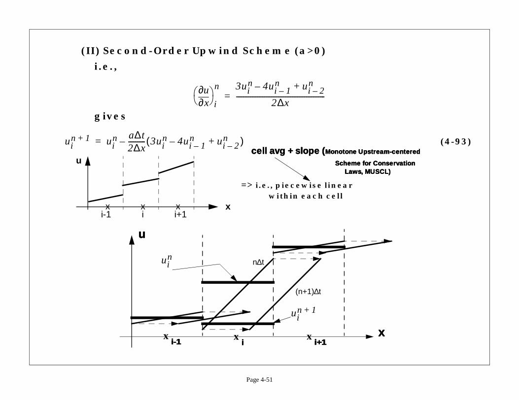
(II) Second-Order Upwind Scheme (a>0)
i.e.,
givesx∂∂u
i
n 3uin 4ui 1–
n ui 2–n+–
2∆x---------------------------------------------------=
uin 1+ ui
n a∆t2∆x---------- 3ui
n 4ui 1–n ui 2–
n+–( )–=
x x xi-1 i i+1
x
u
=> i.e., piecewise linear within each cell
cell avg + slope (cell avg + slope (cell avg + slope (cell avg + slope (Monotone UMonotone UMonotone UMonotone U
Scheme Scheme Scheme Scheme Laws Laws Laws Laws
n∆t
(n+1)∆t
uin
uin 1+
x i-1 i-1 i-1 i-1
uuuu
x i i i i
x i+1 i+1 i+1 i+1
e
iscontinuity
(4-94)
order upwind
Scheme
Page 4-52
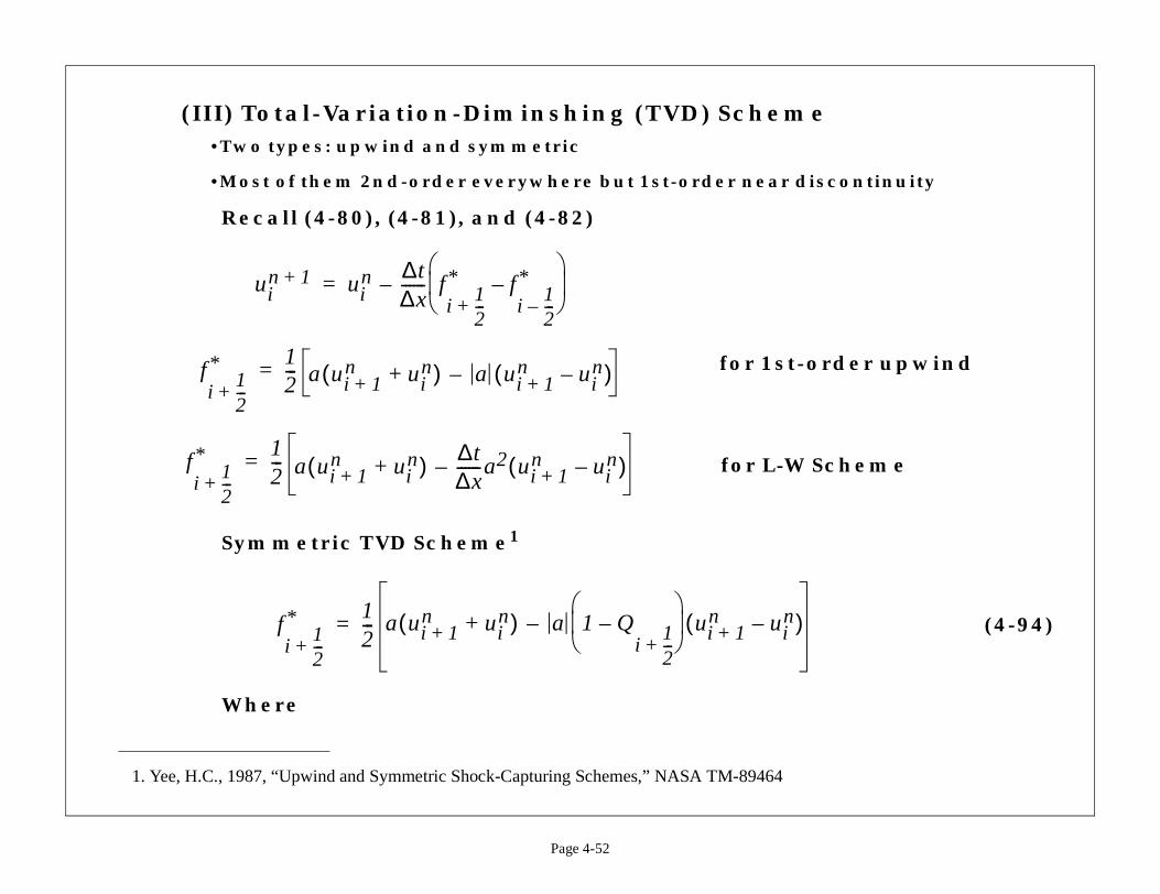
(III) Total-Variation-Diminshing (TVD) Schem•Two types: upwind and symmetric
•Most of them 2nd-order everywhere but 1st-order near d
Recall (4-80), (4-81), and (4-82)
Symmetric TVD Scheme1
Where
1. Yee, H.C., 1987, “Upwind and Symmetric Shock-Capturing Schemes,” NASA TM-89464
uin 1+ ui
n ∆t∆x------ f
i12---+
* fi
12---–
*–
–=
fi
12---+
* 12--- a ui 1+
n uin+( ) a– ui 1+
n uin–( )=
fi
12---+
* 12--- a ui 1+
n uin+( ) ∆t
∆x------a2– ui 1+
n uin–( )=
for 1st-
for L-W
fi
12---+
* 12--- a ui 1+
n uin+( ) a 1 Q
i12---+
–
– ui 1+n ui
n–( )=
(4-95)
ui 2+ ui 1+–
ui 1+ ui–-------------------------------=
1–
12---
u ∆i
32---+
u,
∆i
12---+
u–
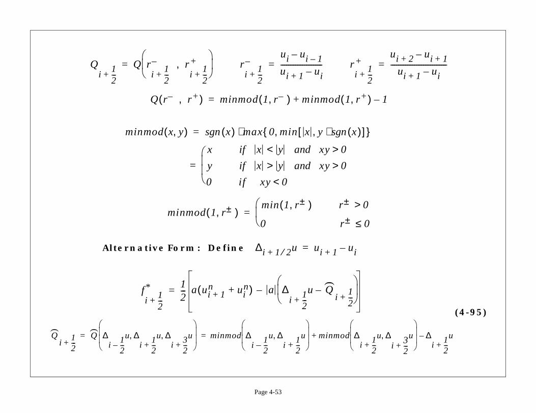
Page 4-53
Alternative Form: Define
Qi
12---+
Q ri
12---+
– ri
12---+
+,
= ri
12---+
–ui ui 1––
ui 1+ ui–-----------------------= r
i12---+
+
Q r– r+,( ) minmod 1 r–,( ) minmod 1 r+,( )+=
minmod x y,( ) x( )sgn max 0 min x y x( )sgn⋅,[ ], ⋅=
x if x y and xy 0><y if x y and xy 0>>0 if xy 0<
=
minmod 1 r±,( )min 1 r±,( ) r± 0>
0 r± 0≤
=
∆i 1 2⁄+ u ui 1+ ui–=
fi
12---+
* 12--- a ui 1+
n uin+( ) a ∆
i12---+
u Qi
12---+
–
–=
Qi
12---+
Q ∆i
12---–
u ∆i
12---+
u ∆i
32---+
u, ,
minmod ∆i
12---–
u ∆i
12---+
u,
minmod ∆i +
+= =)
) )
uation
(4-96)
(4-97)Eu2
2-----=
x
x
InitialProfile
compression
Page 4-54
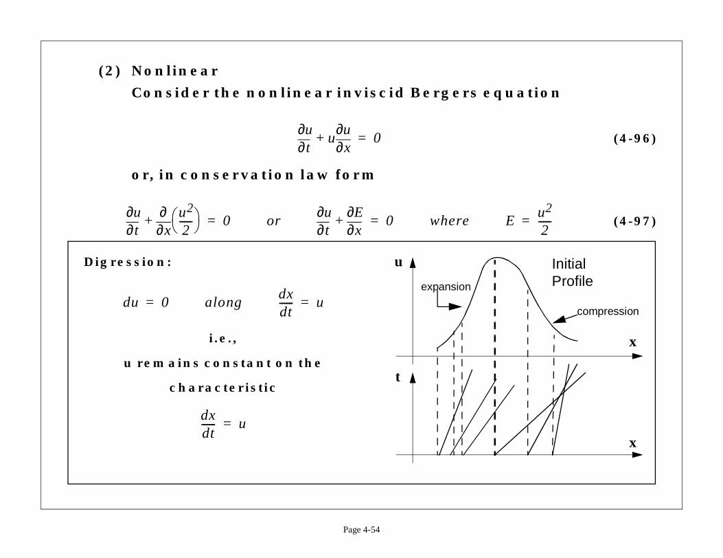
(2) Nonlinear
Consider the nonlinear inviscid Bergers eq
or, in conservation law form
t∂∂u
ux∂∂u
+ 0=
t∂∂u
x∂∂ u2
2----- + 0= or
t∂∂u
x∂∂E
+ 0= where
Digression:
i.e.,
u remains constant on the
characteristic
du 0= alongdxdt------ u=
dxdt------ u=
t
u
expansion
(4-98)
(4-99)
iemann invariant)
(4-100)
ui 1–n
--------------
u∂∂E
u=i
n????
i12---+
n . .??
Page 4-55
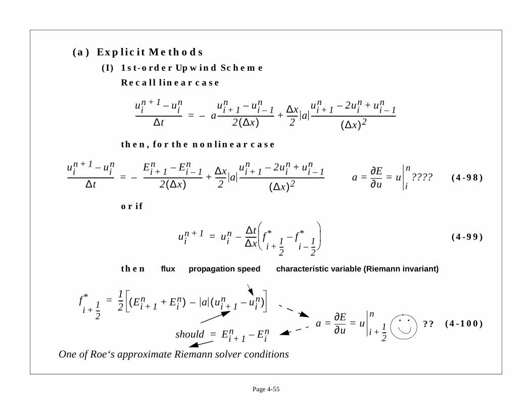
(a) Explicit Methods(I) 1st-order Upwind Scheme
Recall linear case
then, for the nonlinear case
or if
then flux propagation speed characteristic variable (R
uin 1+ ui
n–
∆t-------------------------- a
ui 1+n ui 1–
n–
2 ∆x( )--------------------------------–∆x2
------ aui 1+
n 2uin +–
∆x( )2---------------------------------+=
uin 1+ ui
n–
∆t--------------------------
Ei 1+n Ei 1–
n–
2 ∆x( )---------------------------------–
∆x2
------ aui 1+
n 2uin ui 1–
n+–
∆x( )2-----------------------------------------------+= a =
uin 1+ ui
n ∆t∆x------ f
i12---+
* fi
12---–
*–
–=
fi
12---+
* 12--- Ei 1+
n Ein+( ) a– ui 1+
n uin–( )=
should Ei 1+n Ei
n–=
One of Roe‘s approximate Riemann solver conditions
au∂∂E
u= =
(4-101)
(4-102)
(4-103)
(4-104)
Ax∂∂E
3]
Page 4-56
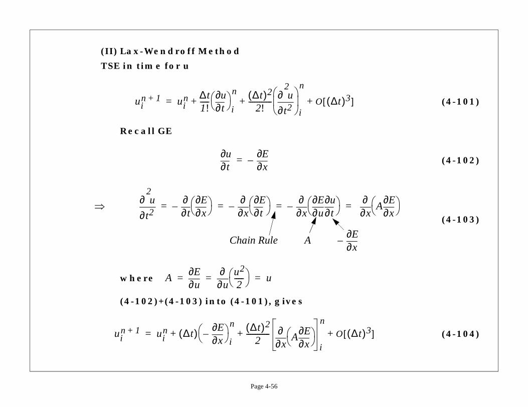
(II) Lax-Wendroff Method
TSE in time for u
Recall GE
where
(4-102)+(4-103) into (4-101), gives
uin 1+ ui
n ∆t1!-----
t∂∂u
i
n ∆t( )22!
-------------t2
2
∂∂ u
i
n
O ∆t( )3[ ]+ + +=
t∂∂u
x∂∂E
–=
⇒t2
2
∂∂ u
t∂∂
x∂∂E –
x∂∂
t∂∂E –
x∂∂
u∂∂E
t∂∂u
–
x∂∂
= = = =
Chain Rule Ax∂∂E
–
Au∂∂E
u∂∂ u2
2----- u= = =
uin 1+ ui
n ∆t( )x∂∂E
–
i
n ∆t( )22
-------------x∂∂
Ax∂∂E
i
n
O ∆t( )[+ + +=
i+3
i12---–
nEi
n Ei 1–n–
∆x--------------------------
---------------------------------------------
Ain+ ) Ei
n Ei 1–n–( )
-----------------------------------------------
Page 4-57
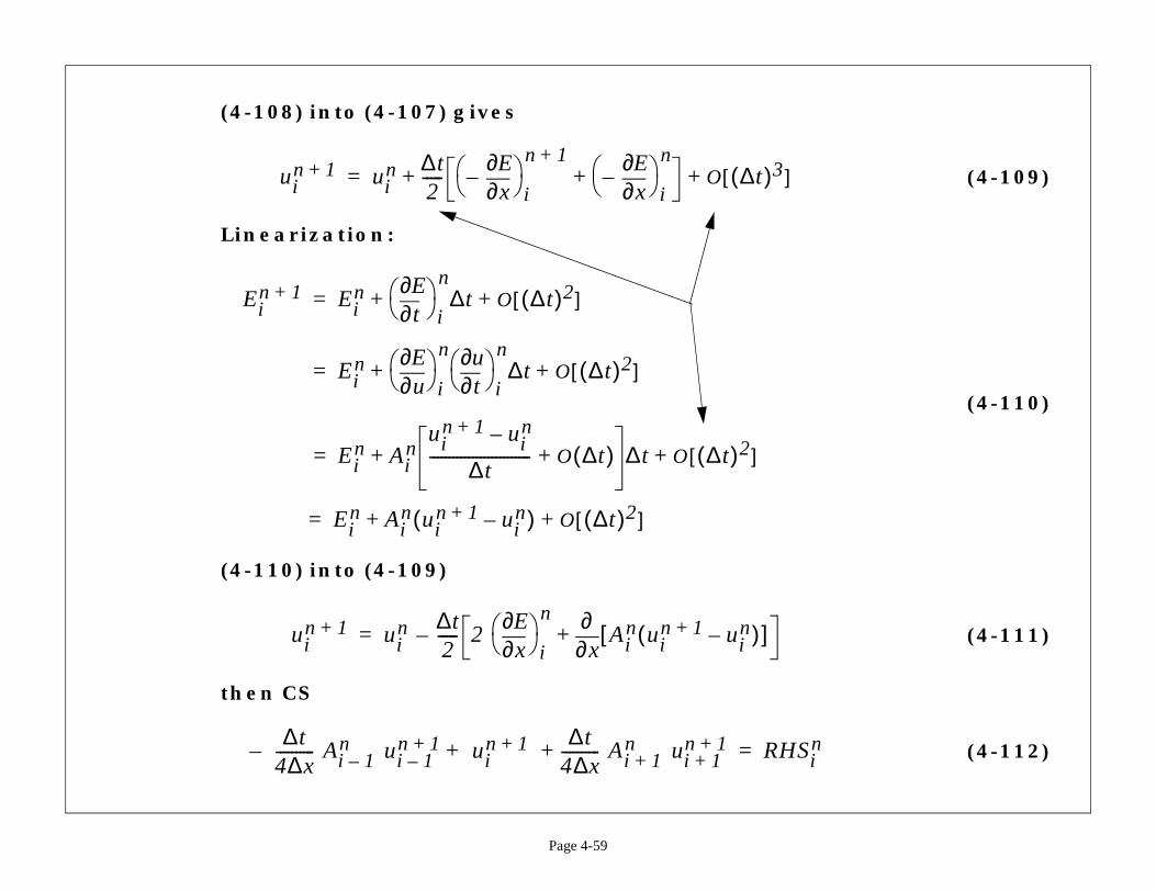
Then CS ==>
Discussions:
•2nd-order method => dispersive
•C. S.,
i-3 i-2 i-1 i i+1 i+2i-1/2 i+1/2
∆x
x∂∂E
i
n Ei 1+n Ei 1–
n–
2∆x---------------------------------=
x∂∂
Ax∂∂E
i
nA
x∂∂E
i12---+
nA
x∂∂E
i12---–
n–
∆x----------------------------------------------------------
Ai
12---+
nEi 1+
n Ein–
∆x--------------------------
A–
∆x------------------------------------------------------= =
⇒x∂∂
Ax∂∂E
i
n12--- Ai 1+
n Ain+( ) Ei 1+
n Ein–( ) 1
2--- Ai 1–
n(–
∆x( )2---------------------------------------------------------------------------------------------=
∆t∆x------ umax 1≤
(4-105)
(4-106)
esult.
cDonald + CN Scheme
(4-107)
(4-108)
Page 4-58
(III) MacCormack Method
Predictor
Corrector
Discussions:
•2nd-order method => dispersive
•C. S., . Local gives better r
(b) Implicit Method - Beam and Warming / Briley and M
CN scheme
Since
ui* ui
n ∆t∆x------– Ei 1+
n Ein–( )=
uin 1+ 1
2--- ui
n ui*+( ) ∆t
∆x------– Ei
* Ei 1–*–( )=
∆t∆x------ umax 1≤ C 1≈
uin 1+ ui
n ∆t2-----
t∂∂u
i
n 1+
t∂∂u
i
n+ O ∆t( )3[ ]+ +=
t∂∂u
x∂∂E
–=
(4-109)
(4-110)
(4-111)
(4-112)in
Page 4-59
(4-108) into (4-107) gives
Linearization:
(4-110) into (4-109)
then CS
uin 1+ ui
n ∆t2-----
x∂∂E
–
i
n 1+
x∂∂E
–
i
n+ O ∆t( )3[ ]+ +=
Ein 1+ Ei
nt∂∂E
i
n∆t O ∆t( )2[ ]+ +=
Ein
u∂∂E
i
n
t∂∂u
i
n∆t O ∆t( )2[ ]+ +=
Ein Ai
nui
n 1+ uin–
∆t-------------------------- O ∆t( )+ ∆t O ∆t( )2[ ]+ +=
Ein Ai
n uin 1+ ui
n–( ) O ∆t( )2[ ]+ +=
uin 1+ ui
n ∆t2-----– 2
x∂∂E
i
n
x∂∂
Ain ui
n 1+ uin–( )[ ]+=
∆t4∆x---------- Ai 1–
n ui 1–n 1+– ui
n 1+ ∆t4∆x---------- Ai 1+
n ui 1+n 1++ + RHS=
., > 2nd-order
(4-113)
(4-114)
equations): LHS
(4-115)
i 1+n ∆t
4∆x---------- Ai 1–
n ui 1–n–
2 ) εe18---≈
εe
Page 4-60
where
Discussions:
•U. S.
•2nd-order method => dispersive
•Linear Damping (should be higher order, i.e
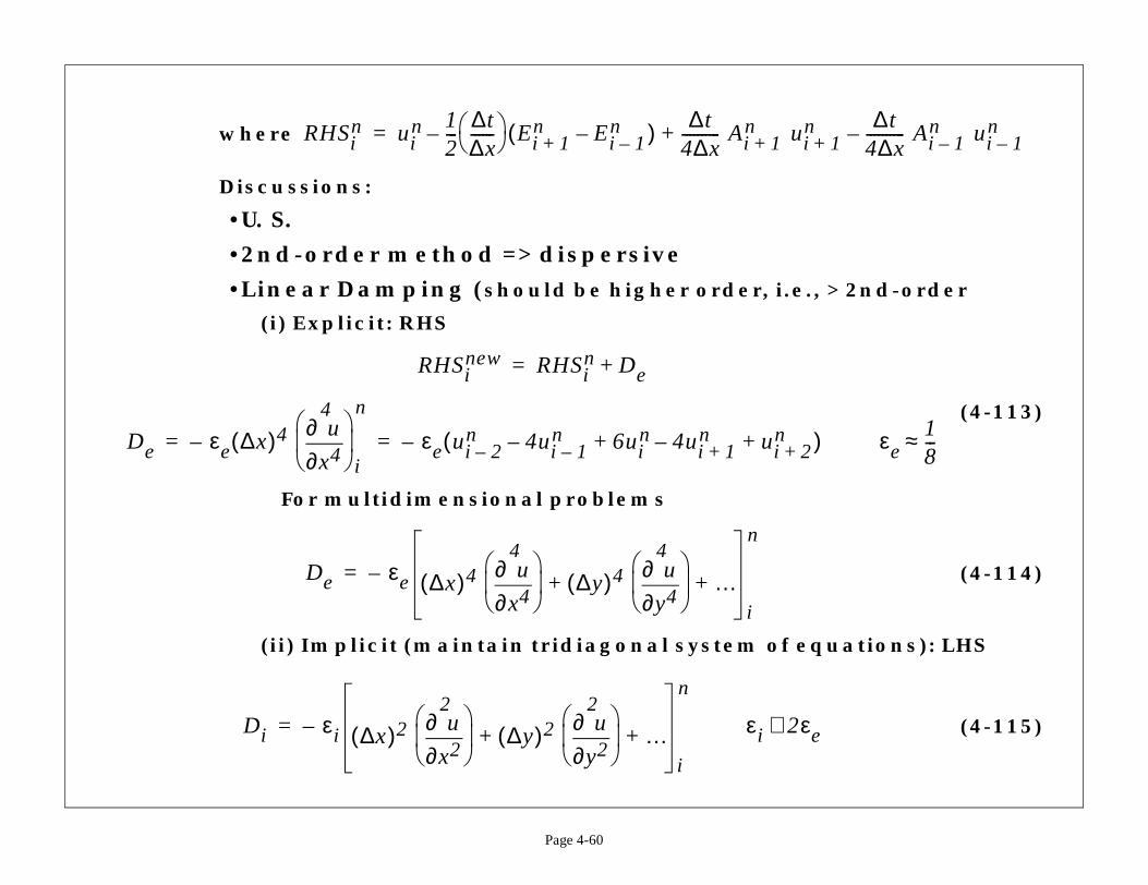
(i) Explicit: RHS
For multidimensional problems
(ii) Implicit (maintain tridiagonal system of
RHSin ui
n 12---∆t∆x------ Ei 1+
n Ei 1–n–( )–
∆t4∆x---------- Ai 1+
n u+=
RHSinew RHSi
n De+=
De εe ∆x( )4x4
4
∂∂ u
i
n
– εe ui 2–n 4ui 1–
n– 6uin 4ui 1+
n– ui +n+ +(–= =
De εe ∆x( )4x4
4
∂∂ u
∆y( )4y4
4
∂∂ u
…+ +i
n
–=
Di εi ∆x( )2x2
2
∂∂ u
∆y( )2y2
2
∂∂ u
…+ +i
n
–= εi 2≅
(4-116)
(4-117)
(4-118)
Ain ui
n 1+ uin–( )[ ]
1–------
1 Ei 1–n– )
Page 4-61
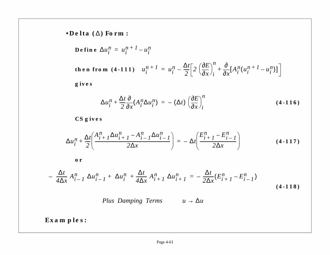
•Delta ( ) Form:
Define
then from (4-111)
gives
CS gives
or
Examples:
∆
∆uin ui
n 1+ uin–=
uin 1+ ui
n ∆t2-----– 2
x∂∂E
i
n
x∂∂
+=
∆uin ∆t
2-----
x∂∂
Ain∆ui
n( )+ ∆t( )–x∂∂E
i
n=
∆uin ∆t
2-----
Ai 1+n ∆ui 1+
n Ai 1–n ∆ui 1–
n–
2∆x--------------------------------------------------------------------
+ ∆tEi 1+
n Ein–
2∆x---------------------------
–=
∆t4∆x---------- Ai 1–
n ∆ui 1–n– ∆ui
n ∆t4∆x---------- Ai 1+
n ∆ui 1+n+ +
∆t2∆x---------- Ei +
n(–=
Plus Damping Terms u ∆u→
(4-119)
x
xu1t u2t
t
nsion
0
Page 4-62
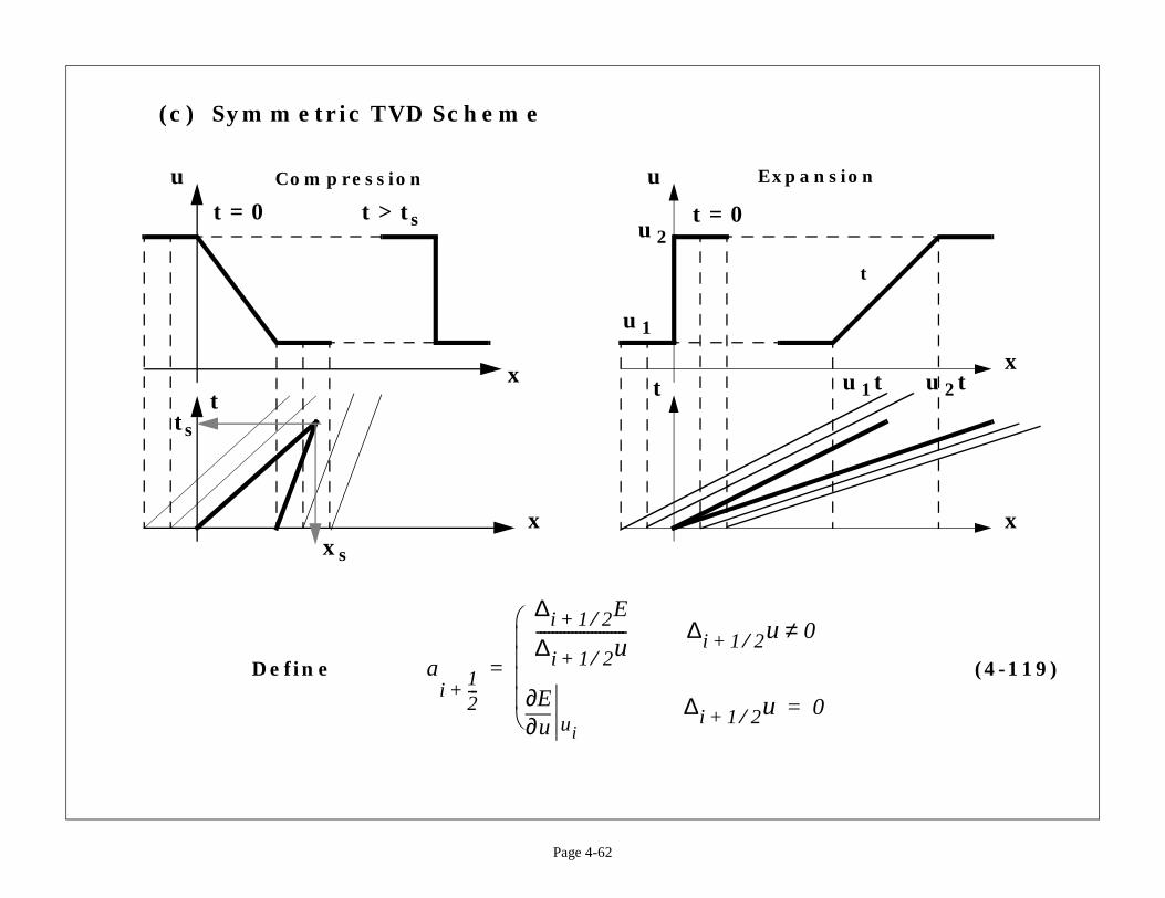
(c) Symmetric TVD Scheme
Define
x
u
x
t t
u
t = 0 t > ts
xs
ts
t = 0
u1
u2
Compression Expa
ai
12---+
∆i 1 2⁄+ E
∆i 1 2⁄+ u----------------------- ∆i 1 2⁄+ u 0≠
u∂∂E
ui∆i 1 2⁄+ u =
=
(4-120)
(4-121)
ui)
12---+
0.125≤
ai
32---+∆
i32---+
u
ai
12---+∆
i12---+
u–
Page 4-63
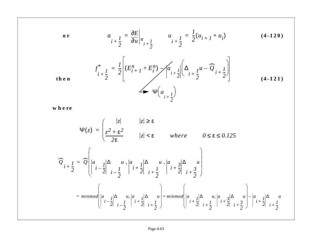
or
then
where
ai
12---+ u∂
∂Eu
i12---+
ui
12---+
12--- ui 1+ +(==
fi
12---+
* 12--- Ei 1+
n Ein+( ) a
i12---+∆
i12---+
u Qi
–
–=
Ψ ai
12---+
)
Ψ z( )z z ε≥
z2 ε2+2ε
----------------- z ε< where 0 ε≤
=
Qi
12---+
Q ai
12---–∆
i12---–
u ai
12---+∆
i12---+
u ai
32---+∆
i32---+
u, ,
=
minmod ai
12---–∆
i12---–
u ai
12---+∆
i12---+
u,
minmod ai
12---+∆
i12---+
u,
+=
) )
(TV)?
(4-122)
(4-123)
governing by the
(4-124)
,
(4-125)
e TVD1.
mes.
1 uin–
Page 4-64
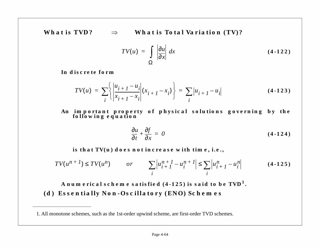
What is TVD? What is Total Variation
In discrete form
An important property of physical solutionsfollowing equation
is that TV(u) does not increase with time, i.e.
A numerical scheme satisfied (4-125) is said to b
(d) Essentially Non-Oscillatory (ENO) Schemes
1. All monotone schemes, such as the 1st-order upwind scheme, are first-order TVD sche
⇒
TV u( )x∂∂u xd
Ω∫=
TV u( )ui 1+ ui–
xi 1+ xi–----------------------- xi 1+ xi–( )
i∑ ui 1+ ui–
i∑= =
t∂∂u
x∂∂f
+ 0=
TV un 1+( ) TV un( )≤ or ui 1+n 1+ ui
n 1+–
i∑ ui +
n
i∑≤
(4-126)
(4-127)
ρw
ρuw
ρvw
w2
p+
et p+ )w
Page 4-65
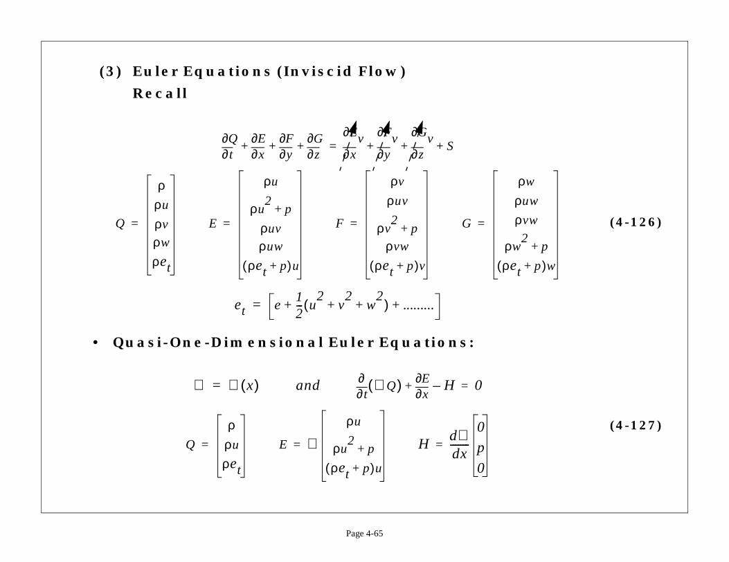
(3) Euler Equations (Inviscid Flow)
Recall
• Quasi-One-Dimensional Euler Equations:
t∂∂Q
x∂∂E
y∂∂F
z∂∂G
+ + +x∂
∂Evy∂
∂Fvz∂
∂GvS+ + +=
Q
ρρu
ρv
ρw
ρet
= E
ρu
ρu2
p+
ρuv
ρuw
ρet p+( )u
= F
ρv
ρuv
ρv2
p+
ρvw
ρet p+( )v
= G
ρρ(
=
et e12--- u
2v2
w2
+ +( ) .........+ +=
ℜ ℜ x( )= andt∂∂ ℜ Q( )
x∂∂E H–+ 0=
Q
ρρu
ρet
= E ℜρu
ρu2
p+
ρet p+( )u
= Hdℜdx--------
0
p
0
=
(4-128)
(4-129)
(4-130)
1Q
n–
t)2]
O ∆t( )2[ ]
O ∆t( )2[ ]+
q2
e1
q2
e2
q2
e3
Page 4-66
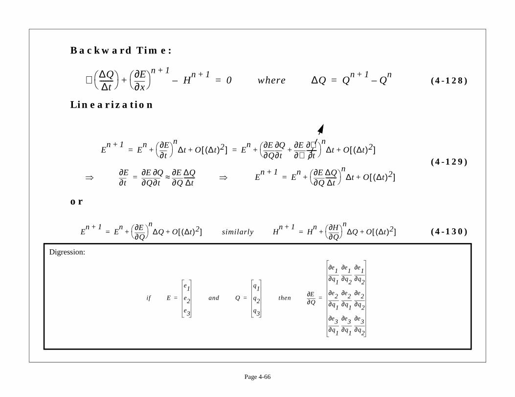
Backward Time:
Linearization
or
ℜ ∆Q∆t--------
x∂∂E
n 1+H
n 1+–+ 0= where ∆Q Q
n +=
En 1+
En
t∂∂E
n∆t O ∆t( )2[ ]+ + E
nQ∂∂E
t∂∂Q
ℜ∂∂E ℜ∂
t∂-------+
n∆t O ∆([+ += =
⇒t∂∂E
Q∂∂E
t∂∂Q
Q∂∂E ∆Q
∆t--------≈= ⇒ E
n 1+E
nQ∂∂E ∆Q
∆t--------
n∆t+ +=
En 1+
En
Q∂∂E
n∆Q O ∆t( )2[ ]+ += similarly H
n 1+H
nQ∂∂H
n∆Q+=
Digression:
if E
e1
e2
e3
= and Q
q1
q2
q3
= thenQ∂∂E
q1∂
∂e1q2∂
∂e1∂
∂
q1∂
∂e2q1∂
∂e2∂
∂
q1∂
∂e3q1∂
∂e3∂
∂
=
(4-131)
(4-132)
obian matrix
2a
2 γ pρ---=
a2
γ γ 1–( )-------------------12---u
2+
A
Page 4-67
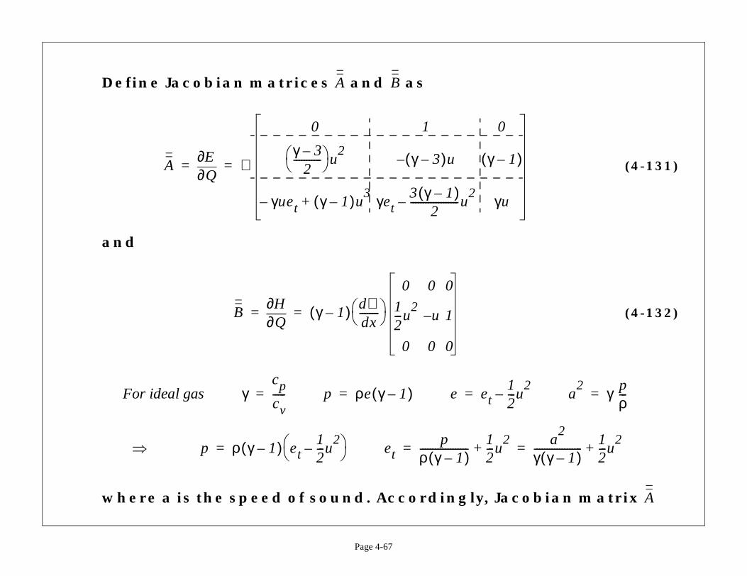
Define Jacobian matrices and as
and
where a is the speed of sound. Accordingly, Jac
A B
AQ∂∂E ℜ
0 1 0
γ 3–2
----------- u
2 γ 3–( )u– γ 1–( )
γuet– γ 1–( )u3+ γet
3 γ 1–( )2
-------------------u2
– γu
= =
BQ∂∂H γ 1–( ) dℜ
dx--------
0 0 0
12---u
2u– 1
0 0 0
= =
For ideal gas γcpcv-----= p ρe γ 1–( )= e et
12---u–=
⇒ p ρ γ 1–( ) et12---u
2–
= etp
ρ γ 1–( )-------------------12---u
2+= =
(4-133)
atrix
(4-134)
(4-135)
A
yperbolic
1 l2 l3 λ1
Page 4-68
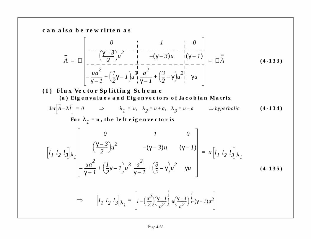
can also be rewritten as
(1) Flux Vector Splitting Scheme(a) Eigenvalues and Eigenvectors of Jacobian M
For = u, the left eigenvector is
A ℜ
0 1 0
γ 3–2
----------- u
2 γ 3–( )u– γ 1–( )
ua2
γ 1–-----------–
12---γ 1– u
3+
a2
γ 1–-----------
32--- γ– u
2+ γu
ℜ= =
det A λ I– 0= ⇒ λ1 u λ2 u a+ λ3 u a–=,=,= h⇒
λ1
l1 l2 l3 λ1
0 1 0
γ 3–2
----------- u
2 γ 3–( )u– γ 1–( )
ua2
γ 1–-----------–
12---γ 1– u
3+
a2
γ 1–-----------
32--- γ– u
2+ γu
u l=
⇒ l1 l2 l3 λ11
u2
2------ γ 1–
a2----------- – u
γ 1–
a2----------- γ 1–( )a2–=
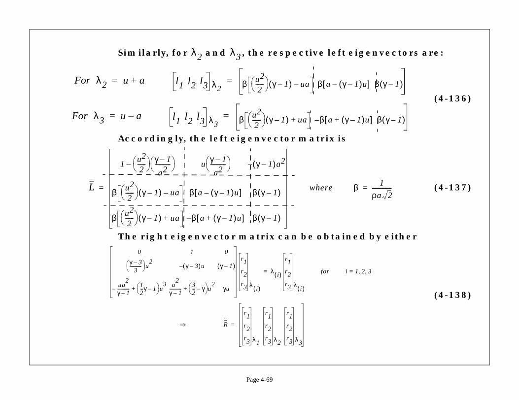
envectors are:
(4-136)
(4-137)
by either
(4-138)
u] β γ 1–( )
)u] β γ 1–( )
1
ρa 2--------------=
2, 3
Page 4-69
Similarly, for and , the respective left eig
Accordingly, the left eigenvector matrix is
The right eigenvector matrix can be obtained
λ2 λ3
For λ2 u a+= l1 l2 l3 λ2β u2
2------ γ 1–( ) ua– β a γ 1–( )–[=
For λ3 u a–= l1 l2 l3 λ3 β u2
2------ γ 1–( ) ua+ β a γ 1–(+[–=
L
1u2
2------ γ 1–
a2----------- – u
γ 1–
a2----------- γ 1–( )a2–
β u2
2------ γ 1–( ) ua– β a γ 1–( )u–[ ] β γ 1–( )
β u2
2------ γ 1–( ) ua+ β a γ 1–( )u+[ ]– β γ 1–( )
= where β
0 1 0
γ 3–3
----------- u
2γ 3–( )u– γ 1–( )
ua2
γ 1–-----------–
12---γ 1– u
3+
a2
γ 1–-----------
32--- γ– u
2+ γu
r1
r2
r3 λ i( )
λ i( )
r1
r2
r3 λ i( )
= for i = 1,
⇒ R
r1
r2
r3 λ1
r1
r2
r3 λ2
r1
r2
r3 λ3
=
(4-139)
(4-140)
rce term
(4-141)
(4-142)
α ρa 2----------=
0=
Page 4-70
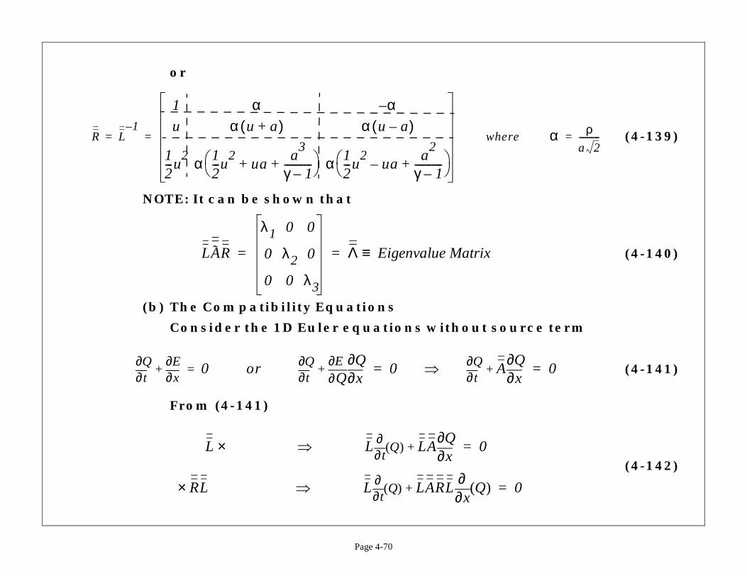
or
NOTE: It can be shown that
(b) The Compatibility Equations
Consider the 1D Euler equations without sou
From (4-141)
R L1–
1 α α–u α u a+( ) α u a–( )
12---u
2 α 12---u
2ua
a3
γ 1–-----------+ +
α 12---u
2ua–
a2
γ 1–-----------+
= = where
LAR
λ1 0 0
0 λ2 0
0 0 λ3
Λ Eigenvalue Matrix≡= =
t∂∂Q
x∂∂E
+ 0= ort∂∂Q
Q∂∂E
x∂∂Q
+ 0t∂∂Q A
x∂∂Q
+⇒=
L × ⇒ Lt∂∂
Q( ) LAx∂∂Q
+ 0=
RL× ⇒ Lt∂∂
Q( ) LARLx∂∂
Q( )+ 0=
omes
(4-143)
(4-144)
(4-145)
(4-146)
Variable Vector
A–
λ3
Page 4-71
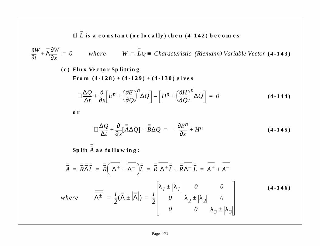
If is a constant (or locally) then (4-142) bec
(c) Flux Vector Splitting
From (4-128) + (4-129) + (4-130) gives
or
Split as following:
L
t∂∂W Λ
x∂∂W
+ 0= where W LQ Characteristic (Riemann)≡=
ℜ ∆Q∆t--------
x∂∂
EnQ∂∂E
n∆Q+ Hn
Q∂∂H
n∆Q+–+ 0=
ℜ ∆Q∆t--------
x∂∂
A∆Q[ ] B∆Q–+En∂x∂
---------– Hn+=
A
A RΛL R Λ+ Λ–+ L R Λ+L RΛ– L+ A+ += = = =
where Λ± 12--- Λ Λ±( ) 1
2---
λ1 λ1± 0 0
0 λ2 λ2± 0
0 0 λ3 ±
= =
(4-147)
(4-148)
(4-149)
(4-150)
(4-151)
Hn
Ei– )n ∆xHi
n–
Page 4-72
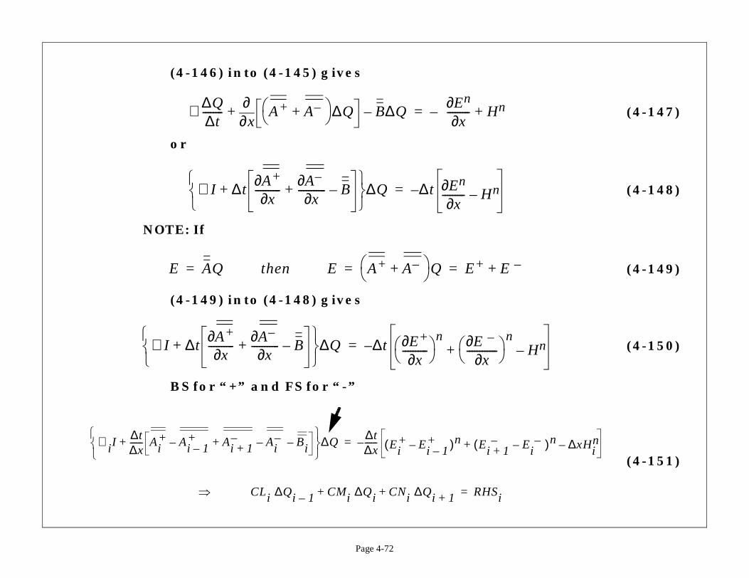
(4-146) into (4-145) gives
or
NOTE: If
(4-149) into (4-148) gives
BS for “+” and FS for “-”
ℜ ∆Q∆t--------
x∂∂
A+ A–+ ∆Q B∆Q–+
En∂x∂
---------– Hn+=
ℜ I ∆tA+∂x∂----------
A–∂x∂----------- B–++
∆Q ∆t En∂x∂
--------- Hn––=
E AQ= then E A+ A–+ Q E+ E –+= =
ℜ I ∆tA+∂x∂----------
A–∂x∂----------- B–++
∆Q ∆t E+∂x∂
---------- n E –∂
x∂------------ n
–+–=
ℜ iI∆t∆x------ Ai
+ Ai 1–+– Ai 1+
– Ai–– Bi–++
∆Q∆t∆x------ Ei
+ Ei 1–+–( )n Ei 1+
– –(+–=
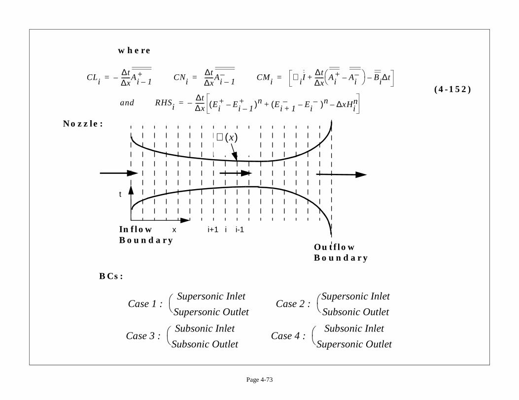
⇒ CLi ∆Qi 1– CMi ∆Qi CNi ∆Qi 1++ + RHSi=
(4-152) Bi∆t–
y
ic Inlet
Outlet
Inlet
Outlet
Page 4-73
where
BCs:
CLi∆t∆x------Ai 1–
+–= CNi∆t∆x------Ai 1–
–= CMi ℜ iI∆t∆x------ Ai
+ Ai––
+=
and RHSi∆t∆x------ Ei
+ Ei 1–+–( )n Ei 1+
– Ei––( )n ∆xHi
n–+–=
Nozzle:
Inflow
Outflow
i+1 i i-1x
t
Boundary
Boundar
ℜ x( )
Case 1 :Supersonic Inlet
Supersonic Outlet Case 2 :
Superson
Subsonic
Case 3 :Subsonic Inlet
Subsonic Outlet Case 4 :
Subsonic
Supersonic
etric Form
(4-153)
(4-154)
l qi
12---+
l–
)
λi
12---+
3
l
λil+ )
Page 4-74
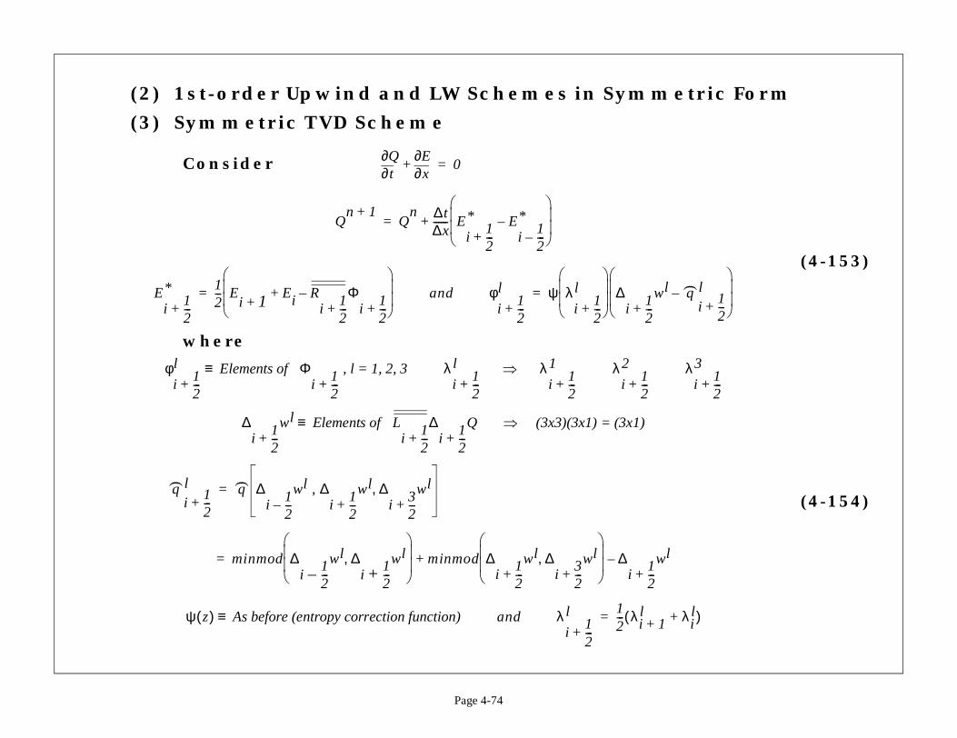
(2) 1st-order Upwind and LW Schemes in Symm
(3) Symmetric TVD Scheme
Consider
where
t∂∂Q
x∂∂E
+ 0=
Qn 1+
Qn ∆t
∆x------ E
i12---+
* Ei
12---–
*–
+=
Ei
12---+
* 12--- E
i 1+Ei R
i12---+Φ
i12---+
–+
= and φi
12---+
l ψ λi
12---+
l
∆i
12---+
w
=
φi
12---+
l Elements of Φi
12---+
, l = 1, 2, 3≡ λi
12---+
l λi
12---+
1⇒ λi
12---+
2
∆i
12---+
wl Elements of Li
12---+∆
i12---+
Q (3x3)(3x1) = (3x1)⇒≡
qi
12---+
l q ∆i
12---–
wl , ∆i
12---+
wl ∆i
32---+
wl,=
minmod ∆i
12---–
wl ∆i
12---+
wl,
minmod ∆i
12---+
wl ∆i
32---+
wl,
∆i
12---+
w–+=
ψ z( ) As before (entropy correction function)≡ and λi
12---+
l 12--- λi 1+
l(=
) )